A maximum likelihood method for fitting colour-magnitude diagrams

Abstract

We present a maximum likelihood method for fitting two-dimensional model distributions to stellar data in colour-magnitude space. This allows one to include (for example) binary stars in an isochronal population. The method also allows one to derive formal uncertainties for fitted parameters, and assess the likelihood that a good fit has been found. We use the method to derive an age of $38.5^{+3.5}_{-6.5}$Myrs and a true distance modulus of $7.79^{+0.11}_{-0.05}$ mags from the $V$ vs $V-I$ diagram of NGC2547 (the uncertainties are 67 percent confidence limits, and the parameters are insensitive to the assumed binary fraction). These values are consistent with those previously determined from low-mass isochronal fitting, and are the first measurements to have statistically meaningful uncertainties. The age is also consistent with the lithium depletion age of NGC2547, and the HIPPARCOS distance to the cluster is consistent with our value.

The method appears to be quite general and could be applied to any N-dimensional dataset, with uncertainties in each dimension. However, it is particularly useful when the data are sparse, in the sense that both the typical uncertainties for a datapoint and the size of structure in the function being fitted are small compared with the typical distance between datapoints. In this case binning the data will lose resolution, whilst the method presented here preserves it.

Software implementing the methods described in this paper is available from http://www.astro.ex.ac.uk/people/timn/tau-squared/.

1 INTRODUCTION

The extraction of astrophysical parameters from colour-magnitude diagrams (CMDs), has been a crucial technique for astronomy since the discovery of the CMD as a diagnostic tool (almost certainly attributable to Hertzsprung, 1911). Since a coeval population of singe stars occupies a curve in a CMD, comparison with theoretical isochrones should allow a determination of global properties of the population such as age, distance and metallicity. Unfortunately such determinations have been hampered by the lack of good statistical methods for carrying out the comparison between observation and theory. For galactic astronomy, the main technique has been a visual comparison of isochrones with the data (although more sophisticated methods have been used for resolved populations in other galaxies). This not only leads to questions of objectivity, but also makes it impossible to derive statistically meaningful uncertainties for parameter estimates.

Were the problem simply fitting a set of datapoints with uncertainties in one dimension (say colour) to a curve then classical $\chi^{2}$ analysis would suffice. Unfortunately a datapoint in colour-magnitude space has uncertainties in both colour and magnitude. (In addition the uncertainties are normally correlated, but as shown by Tolstoy & Saha, 1996, this can be overcome by transforming the problem into a magnitude-magnitude space.) This problem can still be solved analytically if the curve is actually a straight line (Nerit et al., 1989, and references therein). Flannery & Johnson (1982) extended this analytical approach to the general case of a curve by a small curvature approximation. Their method has been used on a significant volume of data, including globular clusters (Borissova et al., 1997; Durrell & Harris, 1993) single-age extra galactic populations (Georgiev et al., 1999) and young ($<$ 10Myr-old) populations (Trullols & Jordi, 1997; Jordi et al., 1996). None of these studies make significant use of the uncertainty measurements, partly because of systematics, but partly there is also the comment that they produce shallow $\chi^{2}$ spaces (Heasley & Christian, 1986) which result in large derived uncertainties (Noble et al., 1991). This is clearly in part because the isochrones do not fit the data well, but may also be a warning that, although one can place clusters in an age sequence by eye, the absolute values of the ages, which must be derived by comparison with the model isochrones, are not as precise as we might hope.

There is a further limitation of the Flannery & Johnson (1982) technique, pointed out most explicitly by Galadi-Enriquez et al. (1998); no population of stars consists entirely of single stars. Unresolved binaries make up a significant fraction of most photometric samples, and are seen as objects which lie up to 0.75 mags brighter than the single star sequence. Indeed, in some coeval populations a distinct equal-mass binary sequence is observed 0.75 mags above the single-star sequence, with unequal-mass binaries lying between the two. Whilst one may be able to extract a single-star sequence by eye and then fit it (Holland & Harris, 1992), clearly the best way is to fit the binaries as well.

Thus one arrives at the fundamental question we address in this paper. If the model is a two dimensional distribution in the colour-magnitude plane, can we derive a statistical test to fit the data to the model? There has been some interest in using Bayesian methods to determine the age of each star in a CMD (Jørgensen & Lindegren, 2005, and references therein), and then using the mean for the cluster age. Although von Hippel et al. (2006) demonstrate such a technique for age determination, it is clear their work will be developed to fit other parameters as well. The problem here, though, is the absence of a goodness-of-fit parameter to choose between isochrones. Another obvious solution is to bin the data into pixels, and compare this with a model. Dolphin (1997) and Aparicio et al. (1997) have developed this technique for large extra-galactic populations, with Dolphin (2002) bringing much of the literature together into a cohesive method. The problem is, however, that our data are often sparse, by which we mean the typical separation of datapoints is large compared with their uncertainties (see Figure 1). Then binning the data simply has the effect of washing out our hard-won photometric precision.

Tolstoy & Saha (1996) developed a technique which does retain the datapoints as points, and which can been seen as a relative of the method we use here. They created simulated observations with a similar number of datapoints to the observed dataset, and then used the distances in colour-magnitude space between the points of the simulated and actual observations as a fitting statistic. Our method, first presented in Naylor & Jeffries (2005), improves on this by using a quasi-continuous 2D distribution as the model, which overcomes problems of sampling the model into a finite number of datapoints, and allows robust uncertainties to be derived.

The method we are proposing is relatively intuitive, so rather than embarking first on a formal analytical proof, we first give the intuitive interpretation (Section 2), and then discuss a numerical experiment which demonstrates the technique using a simulated observation, allowing us to conclude that it recovers the correct answer and uncertainties (Section 3). The formal proofs are in Sections 4 and 5, and the details of practical implementation in Section 6. We draw all the work together in an example using real data in Section 7, before reaching our conclusions in Section 8. An alternative to reading the paper in this order would be to gain a working understanding from Sections 2, 3, and 7, and try the worked examples available with the software fromhttp://www.astro.ex.ac.uk/people/timn/tau-squared.

2 AN INTUITIVE INTERPRETATION

Figure 1: A simulated observation of a 40 Myr-old cluster. See text for details.

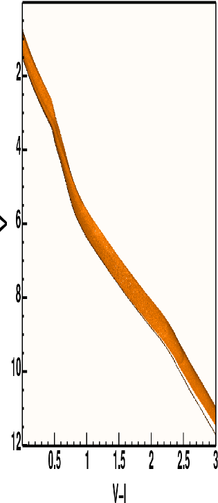
Figure 2: The expected distribution of datapoints underlying the simulation in Figure 1.

Figure 1 shows a simulated observation of 100 stars drawn from a 40 Myr isochrone from D’Antona & Mazzitelli (1997), henceforth referred to as the DAM97 isochrones. As for all the isochrones used in this paper we have converted the isochrones from effective temperature to colour-magnitude space using the relationships derived from fitting the Pleiades (see Jeffries et al., 2001, for details). The cluster is assumed to be unreddened and at a distance modulus of zero. The underlying power law mass function (d$N$/d$M\propto M^{-2.1}$) has been chosen to give a reasonable spread of stars over the magnitude range chosen. We have assumed that 50 percent of the objects are unresolved binaries, but that there are no higher order multiples. Ignoring the higher order multiples should be a small effect since only about 5 percent of systems have more than two members (Duquennoy & Mayor, 1991). The masses of the secondary stars for the binaries are uniformly distributed between the primary star mass and the lowest mass available in the DAM97 models. This is equivalent to assuming the mass-ratio distribution is flat. Whilst there are many claims for structure in the distribution, after selection effects have been taken into account it is hard to argue that a flat distribution is inconsistent with the data (e.g. Mazeh et al., 2003). In addition, as we shall show later the binary fraction, and by implication mass ratio distribution, has little effect on the parameters derived from the fits. The presence of a low-mass cut-off in the DAM97 isochrones leads to the empty wedge between the single star sequence and the more equal-mass binaries visible below $V=9$ in Figure 2. Stars in the wedge would represent binaries where the secondary star lies below the lowest mass available in the models, and hence no stars can be placed in this region. We shall show in Section 7.3 that the wedge has a negligible effect on our derived parameters.

Figure 2 shows the same model, but this time used to generate many more objects, creating a surface density in colour-magnitude space. (For ease of display we have it renormalised such that the integral along each horizontal row is one, but will ignore this renormalisation in what follows). Were there no uncertainties in each datapoint, the relative probability of there being a datapoint at some point $i$ at $(c_{i},m_{i})$ is simply the value of Figure 2 at $(c_{i},m_{i})$, which we refer to as $\rho(c_{i},m_{i})$. Thus each datapoint has an associated value of $\rho$, and if we multiply all these together, the resulting product, $D$ can be used as a fitting statistic. However, in analogy with $\chi^{2}$ we use $-2{\rm ln}D$, which we call $\tau^{2}$. One can then consider moving the model around the plane in colour and magnitude (or perhaps distance and reddening), until the value of $D$ is maximised, or $\tau^{2}$ is minimised.

Introducing uncertainties for each datapoint does not have a large impact on the method. We introduce a two-dimensional uncertainty function for each datapoint, which we call $U_{i}$ (for definiteness, one could consider this to be a two-dimensional Gaussian). One must now consider an uncertainty function centred at $(c_{i},m_{i})$, and then integrate the product of $U$ and $\rho$ (the probability distribution of Figure 2), to obtain a probability $P_{i}$. We then calculate $\tau^{2}$ as $-2\prod{\rm ln}{P_{i}}$. In fact, probably the most difficult problem is introduced by the nature of the astronomical data; since the uncertainties in, say $V$ and $V-I$ are correlated, we must actually integrate under two dimensional Gaussians whose axis is skewed with respect to the colour-magnitude grid (see Section 6.2).

It should be obvious from the above that this is a maximum likelihood method. As such it can be viewed as either Bayesian, or conventional frequentist statistics. As we discussed in the introduction it can be viewed as generalising the method of Tolstoy & Saha (1996) to a model which provides a continuous distribution. As we shall show in Section 5.1, it can also be viewed as a generalisation of $\chi^{2}$.

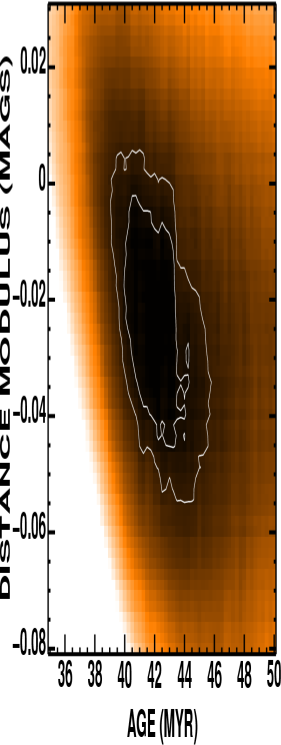
Figure 3: The $\tau^{2}$ space resulting from fitting the simulated observation in Figure 1 (see Section 3.3). The values of $\tau^{2}$ are linearly scaled, and the white lines are contours at the 67 percent ($\tau^{2}=317.3$) and 95 percent ($\tau^{2}=322.8$) confidence levels.

3 A NUMERICAL EXPERIMENT

Our numerical experiment was to find the age and distance modulus of the artificial cluster described in Section 2 from the simulated observation we described. We followed the classical statistical path of finding the best fit to the data, and hence derived estimated parameters (Section 3.1). We then assessed whether this was a good fit (Section 3.2), and then on the assumption it was, derived uncertainties in our fitted parameters (Section 3.3).

3.1 Fitting and parameter estimation

We compared our 100 datapoint simulated observation with a series of model distributions with ages around 40Myr. The model distributions we tested against used the same binary fraction (50 percent) as the original simulation, and the same uniform mass-ratio distribution. We could have also used the same mass function as we used for the simulation. However, to do so would make this a highly unrealistic simulation of fitting real data. In practice, for deriving ages and distances the mass function is a nuisance parameter. Whilst one may think that a simple power-law could be assumed over the mass-range of interest, this would then have to be convolved with the (often unknown) mass-dependent membership selection criteria. For example, in Section 7 we shall use an X-ray selected sample to determine the age of NGC2547, and the precise effect of X-ray selection is unclear. We therefore normalise our model distributions to have a constant number of stars per unit magnitude (e.g. Figure 2). We refer to this procedure as “normalising-out” the mass-function, and will discuss its implications in detail in Section 6.3.3. For datasets with well understood membership selection criteria our procedures can, in principle be simplified by removing the normalising-out of the mass-function, allowing the mass function to be derived as well.

We tested several different offsets in magnitude for each age, which yielded the $\tau^{2}$ space shown in Figure 3. There is a minimum at 42.5Myr, a distance modulus of -0.0195 and $\tau^{2}=311.9$, which is close to the values of 40Myr and 0.0 mags of the artificial cluster from which the simulated observation was drawn.

3.2 Goodness-of-fit

In the case of $\chi^{2}$ fitting one uses the $F$-test, which in essence is a prediction of the cumulative distribution of $\chi^{2}$. We reject fits with $P_{r}(\chi^{2})$ below some critical value, e.g. 5 percent. (We use $P_{r}(x)$ throughout the paper to signify the probability that a statistic exceeds the value $x$. The subscript $r$ differentiates it from $P$, the probability density in the colour-magnitude plane after applying the uncertainty function.) It turns out that numerical integration allows us to predict, after the fit is complete, the expected distribution of $\tau^{2}$ (Section 6.3.1), and thus assess the goodness of fit. Such a distribution is the smooth curve in Figure 4. For the example given we expect our value of $\tau^{2}=311.9$ to be exceeded in 34 percent of fits. We can also normalise $\tau^{2}$ in a similar way to $\chi^{2}$ (for a large number of degrees of freedom) by dividing by the value we expect to be exceeded 50 percent of the time, which in this case gives a reduced $\tau^{2}$, of $\tau_{\nu}^{2}=1.02$.

We can check that this is correct by creating a further 100 simulated observations, and examining the range of $\tau^{2}$ this produces. Figure 4 shows (as a histogram) the distribution of $\tau^{2}$ for from the 100 simulations. The simulations suggest that 21 percent of observations would exceed $\tau^{2}=311.9$; clearly smaller than the 35 percent our theory yields. The reason for the difference is our normalising out of the mass-function (see Section 6.3.3). Despite this (which is a fundamental limit of the data, not of the $\tau^{2}$ test), our method of calculating $\tau^{2}$ is good enough to show that the fit is good, and of course relative values remain useful for testing different models.

Figure 4: The smooth curve is the expected distribution of the probability of obtaining a given $\tau^{2}$ calculated for the simulated observation (using the best fit model) in the way described in Section 6.3.1. The histogram is the distribution of $\tau^{2}$ obtained by fitting 100 further simulated observations generated in the same was as the first.

3.3 Uncertainties for the parameters

The simplest method of estimating the uncertainties would be to create simulated datasets starting with the parameters derived from the observation. However, our normalising out of the mass-function precludes us from doing this. We therefore produce bootstrap datasets by moving each datapoint at constant magnitude onto the best-fit isochrone, and then adding to the two magnitudes a random offset drawn from a population with the appropriate Gaussian distribution for the error bars associated with the datapoint. Since there is not a unique isochronal colour associated with each magnitude (because of the effects of binarism), we have to assign the datapoint to a position in colour using the relative likelihood of each colour drawn from the model. Hence we have assumed that the probability of any given combination of parameters being the correct one is identical to the probability of obtaining those parameters if the underlying model was actually the best-fitting model. We then make 100 bootstrap datasets, and examine the resulting values of the derived parameters, using the RMS about the mean value as the uncertainty. This gives uncertainties in distance modulus and age of 0.012 mags and 1.1 Myr respectively.

We can test these estimates of the uncertainties using the 100 simulated observations we created for Section 3.2. These give a scatter in distance modulus and age of 0.011 mags and 0.9 Myr, in good agreement with our bootstrap method for determining the uncertainties.

In practice, we are interested in more than the simple uncertainties, as there is a correlation between distance modulus and age. We deal with this in an analogous way to $\chi^{2}$ fitting by drawing a contour in the $\tau^{2}$ space which encloses a given fraction of the probability of where the solution lies. We take the values of the distance modulus and age derived from each bootstrap dataset, and find the corresponding value of $\tau^{2}$ in our $\tau^{2}$ space derived from the first simulated observation (Figure 3). (Not the value of $\tau^{2}$ given by the fit to the bootstrap datasets.) This allows us to draw the contour at constant $\tau^{2}$ (317.3) which encloses 67 percent of the derived values, i.e. a “1$\sigma$” confidence limit. This is plotted in Figure 3 and shows the expected correlation between age and distance modulus.

Again we can test this using our simulated observations from Section 3.2. We take the values of the distance modulus and age derived from each simulation, and find the values associated with them from the $\tau^{2}$ space derived from the first simulated observation. 67 percent of them lie below $\tau^{2}$=317.9. Given that we have 100 simulations, we actually require the $\tau^{2}$ below which 67 percent of some large parent population lies, which we estimate is between 317.2 and 318.1. This range which includes the value derived using our proposed technique, implying that technique is correct.

We also tried using a more traditional bootstrap method (e.g. Wall & Jenkins, 2003). For such a bootstrap to work the values of the datapoints (or in our case the values calculated from them) must be identically distributed (see for example Section 15.6 of Press et al., 1992). It is quite clear that the ages and distance moduli derived from each datapoint are not identically distributed, but the traditional bootstrap often works sufficiently accurately even when this assumption is quite strongly violated. To see if this was the case, we created 100 new data sets by randomly selecting 100 points from the original data. (Thus, as is normal in such a bootstrap method, a significant fraction of the datapoints in each realisation are the same.) We found the RMS for each parameter using this dataset, which yields uncertainties of 1.2 Myr and 0.011 mags. Again, these are consistent with those calculated using our method. However, we found that the suggested 67 percent confidence contour for $\tau^{2}$ is too low (314.7). To check that this failure of the traditional bootstrap was not due to our normalising out the mass function we performed a similar simulation using models which retained the mass function. Again we found our bootstrap gave a similar confidence interval to that implied by many simulated observations of the same “cluster”, but in this case the traditional bootstrap overestimated the uncertainties. Clearly the derived parameters from each datapoint are not sufficiently close to identically distributed for the traditional bootstrap to work.

3.4 Conclusion

In this section we have validated the $\tau^{2}$ test by simulating a dataset and recovering the original parameters. We have also shown that we can estimate reliable uncertainties in the measured parameters by creating bootstrap datasets. The “base” for the simulations is created by moving each point in colour space until it lies on the isochrone. By examining the range of $\tau^{2}$ the values of the parameters derived from these datasets, we can estimate confidence intervals analogous to those used in $\chi^{2}$ analysis.

4 FORMAL DEFINITION

Figure 5: A schematic showing a sequence $S$, an observed datapoint $i$ and a point $M$ which may be its position unperturbed by observational error.

Having shown by numerical experiment that $\tau^{2}$ can work, we must now put it on a formal mathematical footing. Figure 5 shows a colour magnitude plane, with a sequence $S$ and an observed datapoint $i$ at $(c_{i},m_{i})$. The datapoint will have an associated two-dimensional probability distribution, which we will assume is Gaussian. This allows us to calculate the probability that the true values of $c$ and $m$ lie within any specified range. Thus if the datapoint lies at ($c_{i},m_{i}$), the probability that the true value lies within an elemental box of area ${\rm}dc\ {\rm d}m$ about $M$ at ($c,m$) can be written as $U_{i}(c-c_{i},m_{i}-m){\rm d}c\ {\rm d}m$, where $U$ is a 2D function which represents the uncertainty for a given datapoint.

We now assume that we have a model $\rho$ which predicts the true density of stars in the colour-magnitude plane. If that model is, say, a $\delta$-function at ($c,m$), then the probability that our data originates from the model is simply the integral of the product of the $\delta$-function and $U_{i}$. More generally, the likelihood for any given datapoint $i$ is given by

$$P_{i}=\int{U_{i}(c-c_{i},m-m_{i})\rho(c,m){\rm d}c\ {\rm d}m}.$$ (1)

If there are $N$ datapoints, the likelihood that the whole distribution originates from the model is the product of the probabilities for each point.

$$D=\prod_{i=1,N}{P_{i}}=\prod_{i=1,N}\int{U_{i}(c-c_{i},m-m_{i})\rho(c,m){\rm d}c\ {\rm d}m}$$ (2)

If we now define $\tau^{2}$ as -2ln$D$, then we arrive at the formal definition of $\tau^{2}$,

$$\tau^{2}=-2\sum_{i=1,N}{\rm ln}\int{U_{i}(c-c_{i},m-m_{i})\rho(c,m){\rm d}c\ {\rm d}m}.$$ (3)

For most practical applications $U_{i}$ has Gaussian uncertainties and is given by

$$U_{i}(c-c_{i},m-m_{i})=e^{-{(c-c_{i})^{2}\over{2\sigma_{c_{i}}^{2}}}-{(m-m_{i})^{2}\over{2\sigma_{m_{i}}^{2}}}},$$ (4)

where $\sigma_{c_{i}}$ and $\sigma_{m_{i}}$ are the uncertainties in each measurement.

There are two obvious interpretations of equation 3. The first is that one has simply taken the model and blurred it by the uncertainties in each datapoint. The likelihood is then simply the product of the values of the model at each point. Alternatively, we have integrated model probability under the 2D Gaussian uncertainty surface. In either interpretation the process of maximising this function to obtain the best fit is analogous to maximising the cross correlation function, though one uses the product rather than the sum of the individual pixel values.

5 SPECIAL CASES

Before using our full two dimensional implementation of $\tau^{2}$ it is useful to reduce Equation 3 for three special cases. These show how (i) $\tau^{2}$ is related to $\chi^{2}$; (ii) that it gives the standard form for fitting a straight line to data with uncertainties in two dimensions; and (iii) that it can also reduce to the same approximation as that of Flannery & Johnson (1982) for curve fitting with uncertainties in two dimensions.

5.1 Curve fitting for data with one dimensional uncertainties

The most important special case to derive is that for when the model predicts that a point whose true value is ($c,m$) should always have an observed value of $c_{i}=c$, but has a range of possible observed values $m_{i}$, represented by a Gaussian probability distribution. In this case $\tau^{2}$ should behave like $\chi^{2}$. Removing the dependence on $c$ from Equations 3 and 4 yields

$$\tau^{2}=-2\sum_{i=1,N}{\rm ln}\int{e^{-{(m-m_{i})^{2}\over{2\sigma_{m_{i}}^{2}}}}\rho(m){\rm d}m}.$$ (5)

Further, for any single datapoint $\rho(m)$ is a $\delta$ function centred on $m$, and with a normalisation we choose to be one, thus

$$\tau^{2}=-2\sum_{i-1,N}{\rm ln}\Big{(}e^{-{(m-m_{i})^{2}\over{2\sigma_{m_{i}}^{2}}}}\Big{)}=\sum_{i-1,N}{(m-m_{i})^{2}\over{\sigma_{m_{i}}^{2}}}.$$ (6)

This is the standard form for $\chi^{2}$ fitting to a function with uncertainties in one dimension. Thus we have shown that $\chi^{2}$ is a special case of $\tau^{2}$, where the model is a curve and the data have uncertainties in one dimension.

5.2 A linear isochrone

We now wish to examine the special case where the probability distribution is a linear sequence, but the data now have uncertainties in both co-ordinates. We have three aims in presenting this special case. First, to show that the standard form for fitting a straight line with uncertainties in two dimensions is a special case of $\tau^{2}$. Second, we will test our (numerical) implementation of $\tau^{2}$ by checking it recovers the same answer as the analytical expression. We find that if this is to be the case we must use the correct normalisation for $\rho$, which we derive below. Finally, there is an intuitive interpretation of the analytical expression which is useful for interpreting the more general case of fitting a curve with uncertainties in both dimensions.

5.2.1 Analytical form

Formally we wish to assess the probability that a point $i$ at ($c_{i},m_{i}$) originates from the isochrone

$$m={{{\rm d}m}\over{{\rm d}c}}c+k,$$ (7)

where $k$ is a numerical constant. We begin by changing to a co-ordinate system ($x,y$), a process shown graphically in Figure 6. We first normalise by the uncertainties in each axis, then place ($c_{i},m_{i}$) at the origin, and finally rotate the system through an angle $\theta_{i}$ such that the x-axis lies parallel to the sequence. (We use the subscript $i$ to emphasize that $\theta$ depends on the uncertainties and so is potentially different for each datapoint.) Thus

$${{m-m_{i}}\over{\sigma_{m_{i}}}} = y{\rm cos}\theta_{i}+x{\rm sin}\theta_{i},$$ (8)

$${{c-c_{i}}\over{\sigma_{c_{i}}}} = x{\rm cos}\theta_{i}-y{\rm sin}\theta_{i}.$$ (9)

Equation 1 then becomes

$$P_{i}=\int{e^{-{{x^{2}+y^{2}}\over 2}}}\rho(x,y){\rm d}x{\rm d}y.$$ (10)

In this co-ordinate system we denote the $y$-distance between the $x$-axis and the sequence $y_{0}$. We can now divide $\rho(x,y)$ into $\rho(x)\rho(y)$ where $\rho(x)$ is constant and $\rho(y)=0$ except where $y=y_{0}$. This allows us to separate the integrals, and find that

$$P_{i} = \int{e^{-{{y_{0}^{2}}\over 2}}e^{-{{x^{2}}\over 2}}\rho(x)\rho(y){\rm d}x{\rm d}y}$$ (11)

$$= e^{-{{y_{0}^{2}}\over 2}}\rho(x)\int{e^{-{{x^{2}}\over 2}}{\rm d}x}\int{\rho(y){\rm d}y}$$ (12)

$$= \sqrt{2\pi}e^{-{{y_{0}^{2}}\over 2}}\rho(x)\int{\rho(y){\rm d}y}.$$ (13)

Now $\rho(x)\int{\rho(y){\rm d}y}$ is the number of objects per unit length in $x$, and in terms of the number of objects per unit magnitude, $\rho(m)$, is $\sigma_{m_{i}}$sin$\theta_{i}\rho(m)$, thus

$$P_{i}=\sqrt{2\pi}e^{-{{y_{0}^{2}}\over 2}}\sigma_{m_{i}}{\rm sin}\theta_{i}\rho(m).$$ (14)

Thus, Equation 3 becomes

$$\tau^{2}=\sum_{i=1,N}{y_{0}^{2}}-2\sum_{i=1,N}{{\rm ln}(\sigma_{m_{i}}{\rm sin}\theta_{i}\rho(m)\sqrt{2\pi}}).$$ (15)

5.2.2 Intuitive interpretation

This equation has an intuitive interpretation, which is especially useful for what follows. The probability that a star at ($c_{i},m_{i}$) originates from a given point on an isochrone is given by the probability that there is a datapoint whose true value lies at that point on the isochrone, multiplied by the probability that the uncertainties could move it to ($c_{i},m_{i}$). For the whole isochrone, therefore, the probability that it will yield a point at ($c_{i},m_{i}$) is given by the line integral along the isochrone, multiplied at each point by the probability of it being moved to ($c_{i},m_{i}$). This probability distribution is (in normalised units) simply a two-dimensional Gaussian distribution centred on ($c_{i},m_{i}$). Any linear cut through such a 2D Gaussian, such as that made by the isochrone, is itself a 1D Gaussian, but with is peak reduced by $e^{-{y_{0}^{2}\over 2}}$ with respect to the 2D distribution. Thus the integral along the line is the integral under this 1D Gaussian. The ratio of the integrals under 1D and 2D Gaussians of equal peak height is $\sqrt{2\pi}$, but this must also be multiplied by the decrease in peak, $e^{-{y_{0}^{2}\over 2}}$, explaining the form of Equation 13.

5.2.3 Testing the linear isochrone

Figure 6: A linear isochrone which makes an angle $\theta$ with axes normalised by the uncertainties in each dimension. The $x$ and $y$-axes define a rotated co-ordinate system parallel with the isochrone, centred on the datapoint ($c_{i}$, $m_{i}$). Note magnitude axis is reversed.

Equation 15 gives us a practicable way of fitting a linear isochrone, by minimising $\tau^{2}$ as a function of $y_{0}$ and the gradient of the isochrone (which is related to $\theta_{i}$). First, if we wish $\tau^{2}$ to reduce to $\chi^{2}$ we must choose the normalisation of $\rho$ in Equation 15. Since $y_{0}$ is distributed as a Gaussian with a standard deviation of one, this means we must ensure the second term is zero. Thus

$$\sum_{i=1,N}{{\rm ln}(\sigma_{m_{i}}{\rm sin}\theta_{i}\sqrt{2\pi}})+\sum_{i=1,N}{\rm ln}(\rho(m))=0,$$ (16)

giving

$$\rho(m)^{-N}=\prod_{i=1,N}(\sigma_{m_{i}}{\rm sin}\theta_{i}\sqrt{2\pi}).$$ (17)

From Figure 6 it is clear that $\theta$ is related to the gradient of the isochrone by

$${{{\rm d}m}\over{{\rm d}c}}={{\sigma_{m_{i}}}\over{\sigma_{c_{i}}}}{\rm tan}\theta_{i}.$$ (18)

The value of $y_{0}$ can be found using the above equation, and setting $x$=0 in Equations 8 and 9, and substituting into Equation 7 to obtain

$$y_{0}={c_{i}\over\sigma_{c_{i}}}{\rm sin}\theta_{i}+{{k-m_{i}}\over{\sigma_{m_{i}}}}{\rm cos}{\theta_{i}}.$$ (19)

For a given linear isochrone and set of simulated datapoints this means we can calculate analytically a value for $\tau^{2}$. We can then use this to test the 2D numerical code we describe below.

5.2.4 Comparison with a straight line fit with 2D uncertainties

Clearly the best-fitting straight line will be obtained by minimising the sum over all datapoints of $y_{0}^{2}$ in Equation 19. We can rewrite the equation such that

$$y_{0}^{2}={{{c_{i}{{{\rm d}m}\over{{\rm d}c}}+k-m_{i}}^{2}}\over{\sigma_{m_{i}}^{2}+\sigma_{c_{i}}^{2}{{{\rm d}m}\over{{\rm d}c}}}}.$$ (20)

This is the standard expression to be minimised for fitting a straight line to data with uncertainties in both co-ordinates (e.g. Nerit et al., 1989), which demonstrates that such fitting is a special case of $\tau^{2}$.

5.3 A real isochrone

We can use the interpretation of Equation 15 presented in Section 5.2.2 to visualize the limit in which the approximation that the isochrone is linear is no longer valid. Once the curvature of the isochrone becomes large compared with the typical uncertainties for a datapoint, then it cannot be approximated to a straight line when the line integral is performed. However, for the case where the curvature is small, one might still be able to use Equation 15, interpreting $y_{0}$ as the distance of closest approach of the line to the datapoint, and $\theta_{i}$ referring to the gradient of the isochrone at closest approach. Although a rather different derivation, such a technique would be identical, save some normalisation factors, to the near-point estimator of Flannery & Johnson (1982).

6 THE TWO DIMENSIONAL APPROACH

6.1 Implementation

We can gain our first insights into the 2D case by reproducing the results from the 1D-linear and 1D-real isochrones of Sections 5.2 and 5.3 using the 2D algorithm.

We evaluate the integral in Equation 3 using a 2D grid. We represent $\rho(c,m)$ as a grid and, for reasons we will discuss later, populate this grid by a Monte Carlo method. For these 1D isochrones we begin by randomly selecting a magnitude, and then assigning a colour according to the isochrone. The value of the appropriate pixel of $\rho(c,m)$ is then incremented by one. At the end of the Monte Carlo we then ensure that $\rho(m)$ is one by dividing each pixel by the sum of all pixels at that magnitude. This means that in practice the initial distribution in magnitude used by the Monte Carlo is unimportant, provided it is smooth.

For each datapoint we can now evaluate Equation 1. We multiply each pixel of $\rho(c,m)$ by Equation 4. In principle, before using $\rho$ we should correct it by the normalisation given in Equation 17. In practice it is simpler to apply a correction to the $\rho$ used for each datapoint, which when the probabilities for each datapoint are multiplied together gives the same effect. Thus for each datapoint we divide $\rho$ by the normalisation factor $\sigma_{m_{i}}{\rm sin}\theta_{i}\sqrt{2\pi}$. To evaluate ${\rm sin}\theta_{i}$ we require the gradient at each pixel, which we evaluate and store at the same time as we calculate $\rho(c,m)$, by differencing the $c$ and $m$ values of the most extreme valued points from the Monte Carlo which lie within the pixel. Of course the gradient is only defined on the isochrone, and we need it for a general point in the CMD. We can be arbitrary about how we make this generalisation, since our normalisation is only there to ensure that if we have a straight line (where the gradient is obviously always the same) we obtain a $\tau^{2}$ of one per datapoint. We therefore choose the gradient for an arbitrary pixel to be that of the isochrone at the magnitude of the pixel. At this point one can test the code is functioning correctly by using a linear isochrone and testing the result for $\tau^{2}$ against the analytical result given in Equation 15.

To move to the more general 2D case one fills the array for $\rho$ by selecting stars randomly according to some mass function. They are assigned companions (or not) according to the preferred binary frequency and mass functions, and then one uses isochrones to place the resulting systems in colour-magnitude space. The remainder of the procedure is as before for the linear isochrone.

6.2 Correlated Uncertainties

A significant issue with any CMD is that the uncertainties are correlated, since a change in, say $V$ also results in a change in $V-I$. Perhaps the most obvious change in formalism to deal with this is that suggested by Tolstoy & Saha (1996), where the actual fitting is carried out in a magnitude-magnitude space. We have found it simpler (and therefore more robust against coding errors) to use colour-magnitude space throughout our code. However, at the point of evaluating Equation 4 one can calculate the argument of the exponential in magnitude-magnitude space, reconstructing the uncertainty in the second magnitude using the uncertainties in magnitude and colour. In principle this allows considerable flexibility, including the ability to deal correctly with data which have been created using a colour term in the transformation from instrumental to apparent magnitude, and a co-efficient other than unity in the transformation from instrumental to apparent colour.

6.3 The distributions of $\tau^{2}$

Once we have fitted our data, to calculate whether it is a good fit we need to know $P_{r}(\tau^{2})$. To calculate this we must first calculate the distribution for a single point, and then calculate the expected distribution for the whole ensemble of datapoints.

6.3.1 The $\tau^{2}$ distribution for one datapoint

To understand the form of the $\tau^{2}$ distribution it is useful to begin by considering a classical $\chi^{2}$ fitting problem, but solved as though it were suitable for $\tau^{2}$. In such a problem the model isochrone is a curve in colour magnitude space, and the uncertainties are treated as 2D Gaussians which are infinitely thin in the colour dimension, and have the correct width in magnitude space to represent the 1D uncertainty. We can calculate the chance that a star at a given point on the sequence actually appears, due to observational error, at a given position on the CMD. If we integrate this along the entire sequence we obtain the probability of there being a datapoint at any given position on the CMD. Since our uncertainties are Gaussian, and the line is a form of $\delta$-function, the distribution of probabilities in the plane is itself Gaussian. Thus, the likelihood of finding a datapoint at given probability, say $P$, is proportional to the fraction of the CMD covered by pixels with that probability, multiplied by $P$. Assuming all pixels have the same area, this can be calculated numerically by summing the values of all pixels for which $P$ lies within a given (infinitesimal) range. Strictly speaking this should only be interpreted in the cumulative sense, i.e. that the probability of finding a datapoint with a probability of $P$ or less is proportional to the fraction of the area covered by each probability less than $P$, multiplied by that probability, and then integrated over all probabilities less than $P$. We, of course, have chosen not to work in probability $P$, but in $\chi^{2}=-2{\rm ln}P$. Thus we have not quoted the chance of a datapoint being at a probability $P$ or less, rather the chance of it lying at a given $\chi^{2}$ or more.

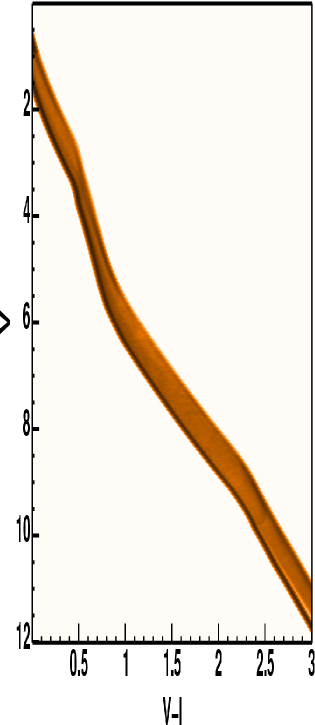
Figure 7: A model created using the DAM97 isochrones, and a binary fraction of 0.5. The uncertainties used are 0.01 mag in each filter.

Of course when we perform this sum over the plane, the resulting distribution will be that of $\chi^{2}$. We can still retain a $\chi^{2}$ distribution in the plane if we make the uncertainties two dimensional, provided we restrict the isochrone to be a straight line. But if the model is to be a curve, and/or include binaries, the distribution of probability in the plane will no longer be Gaussian, and the probability of exceeding a given value will no longer behave like $\chi^{2}$. We can still accurately predict the distribution of values of $-2{\rm ln}P$ we expect to get. That is obtained by simply creating a histogram of the probabilities from an image such as that in Figure 7. But, this will no longer be distributed as $\chi^{2}$, and to emphasize this fact we will now refer to $-2{\rm ln}P$ as $\tau^{2}$.

Figure 8: The $\tau^{2}$ distribution (the probability of exceeding a given $\tau^{2}$ from the DAM97 isochrones using two different values of the uncertainty. A $\chi^{2}$ distribution for one degree of freedom is shown for comparison.

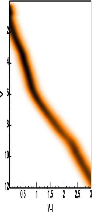
Figure 9: A model created using the DAM97 isochrones, and a binary fraction of 0.5. The uncertainties used are 0.1 mag in each filter. The feature at bright magnitudes is caused by the upper cut-off in mass for the DAM isochrones. At this cut-off the binary sequence rises to brighter magnitudes than the single star sequence. When the single-star sequence ends, the smoothed sequence moves redwards.

In Figure 8 we show the cumulative distribution for the value of $\tau^{2}$ taken from Figure 7, where the uncertainties are 0.01 magnitudes in each filter. When compared with the $\chi^{2}$ distribution for one degree of freedom, there are two major differences between $\tau^{2}(\sigma=0.01)$ and $\chi^{2}$. First $\tau^{2}(\sigma=0.01)$ has no values below about 1, and second it falls much more slowly. The slow fall is the effect of the “plateau” region between the single and binary star sequences, which contributes a large area of low probability, and hence high $\tau^{2}$. The absence of values below about one is the result of our requirement that $\rho(m,c)$ at a given magnitude integrates to one over all colours. This imposes a maximum value on $P$, and hence a minimum on $\tau^{2}$. As one moves to larger uncertainties ($\tau^{2}(\sigma=0.1)$ in Figure 8), these differences become less pronounced. The change from $\tau^{2}(\sigma=0.01)$ to $\tau^{2}(\sigma=0.1)$ shows that as the uncertainties become larger, $\tau^{2}$ tends to $\chi^{2}$. The reason for this is clear if one compares Figure 7 with Figure 9. As the uncertainties become large compared with the distance between the single and binary star sequences, we can approximate them to a single sequence.

6.3.2 The $\tau^{2}$ distribution for many datapoints

Having calculated $\tau^{2}$ for a single datapoint, it would appear straightforward to calculate it for an ensemble. We will do this by comparison with the case for $\chi^{2}$.

Figure 10: The two-dimensional differential probability distribution of $\chi$. The contours are evenly spaced starting at a probability of zero. Note that the axes are in $\chi$ not $\chi^{2}$.

Figure 11: A two-dimensional differential probability distribution of $\tau$ for the DAM97 isochrones and uncertainties of 0.01 mag (horizontal axis) and 0.1 mag (vertical axis). The contours are evenly spaced starting at a probability of zero. Note that the axes are in $\tau$ not $\tau^{2}$.

The standard proof for the $\chi^{2}$ distribution for many datapoints is a generalization of the proof for just two (e.g. Saha, 1995). One considers a two-dimensional space, with $\chi_{1}$ (not $\chi^{2}_{1}$) as one axis and $\chi_{2}$ as the other. At each point in the space one evaluates the probability of obtaining simultaneously values of $\chi_{1}$ between $\chi_{1}$ and $\chi_{1}+d\chi_{1}$ and of $\chi_{2}$ between $\chi_{2}$ and $\chi_{2}+d\chi_{2}$. This probability is simply ${{dP_{r}}\over{d\chi_{1}}}{{dP_{r}}\over{d\chi_{2}}}$, or in more familiar terms of the differential probability distribution of $\chi^{2}$, $4\chi_{1}\chi_{2}{{dP_{r}}\over{d\chi^{2}_{1}}}{{dP_{r}}\over{d\chi^{2}_{2}}}$. This function is plotted in Figure 10 using $P_{r}(\chi^{2})$ for one degree of freedom. The figure shows that the probability of obtaining any given value of $\chi^{2}=\chi^{2}_{1}+\chi^{2}_{2}$ is independent of the value of either $\chi^{2}_{1}$ or $\chi^{2}_{2}$. This allows the proof for $\chi^{2}$ to proceed to its conclusion that the probability of obtaining any given value of $\chi^{2}$ is proportional to $\chi_{1}{{dP_{r}}\over{d\chi^{2}_{1}}}$ times the length of the arc at a radius $\chi^{2}$ (or more generally the area of the N-dimensional surface). The crucial point here is the interpretation that the probability of obtaining a given $\chi^{2}$ is simply the line integral of the probability along a line of constant $\chi^{2}$. For $\chi^{2}$ the integral can be performed analytically, because the probability is the same along a line of constant $\chi^{2}$; this is not the case for $\tau^{2}$, and in this case the integral must be evaluated numerically.

Figure 11 shows the equivalent plot to Figure 10, but instead of $\chi^{2}=\chi^{2}_{1}+\chi^{2}_{2}$ we have $\tau^{2}=\tau^{2}(\sigma=0.01)+\tau^{2}(\sigma=0.1)$, for the DAM97 isochrones. Before embarking on how to use this plot to determine the probability of obtaining a given $\tau^{2}$ or greater, it is useful to understand the differences between Figures 10 and 11. The most likely value of $\chi$ is zero, simply because the most probable position for a datapoint to lie at its value before perturbation by observational error. For $\tau$ this is not the case. At any given value of (say) $V$, there are a range of actual $V-I$ values it could have originated from. Furthermore, the large area of the CMD covered by binaries (albeit at a low probability), gives a very large chance that a star will yield a high $\tau$. This point can be emphasised in two ways. First, collapsing the plot onto the y-axis gives the differential version of the upper curve in Figure 8, with its emphasis on high values of $\tau^{2}$. Second, collapsing the curve onto the x-axis yields a distribution more strongly skewed to low values, as one would expect because the larger value of $\sigma$ causes the distribution to tend towards that for $\chi^{2}$.

The problem with Figure 11, from the point-of-view of evaluating $P_{r}(\tau^{2})$ is that ${d^{2}P_{r}}\over{d\tau_{1}d\tau_{2}}$ along a line of constant $\tau^{2}$ is not independent of either $P_{r}(\tau^{2}(\sigma=0.01))$ or $P_{r}(\tau^{2}(\sigma=0.1))$. This precludes us using the analytical $\chi^{2}$-method to evaluate $P_{r}(\tau^{2})$. However, this does not stop us undertaking a numerical line integration along fixed curves of $\tau^{2}$ to evaluate the probability of exceeding that value of $\tau^{2}$. The route we have followed to perform this numerical integration relies on the fact that the arc length is proportional to the number of pixels. One can calculate a grid of the differential probability (i.e. the probability of obtaining a certain $\tau^{2}$, not of exceeding it), akin to Figure 11 by simply multiplying the two differential distributions together. A simple histogram of the number of pixels with a given value of $\tau^{2}$ is then ${dP_{r}}\over{d\tau^{2}}$. Unfortunately, when one generalizes this to say, the 100 dimensions needed for a 100 point dataset, the calculation becomes intractable in reasonable computation times. We therefore perform the calculation dimension by dimension. We take the first two $\tau^{2}$ distributions, and multiply each point in one distribution by every other point in the other. We then bin the result into bins of $\tau^{2}=\tau^{2}_{1}+\tau^{2}_{2}$ to produce a new, one dimensional distribution. This can then be multiplied by the next dimension, and the process repeated until all dimensions have been allowed for. We then integrate this to change from a differential to a cumulative distribution.

6.3.3 $\tau_{\nu}^{2}$ and practicalities

The method described thus far is very general, with little tailoring to the specific problems of CMDs. In calculating the expected distribution of $\tau^{2}$ however, we must return to the subject of normalising-out the mass function, a procedure first discussed in Section 3.1. If the model for Figure 2 included a mass function with increasing numbers of stars at fainter magnitudes, we would expect to see a much higher probability density in the bottom part of the plot than in the top part. Since we expect the majority of our datapoints to lie at faint magnitudes, this is perfectly correct. The best $\tau^{2}$ values will be found by placing the majority of the points in the regions of highest probability density; thus the mass function is a driving force in the fitting procedure. Note, however, that the distribution of $\tau^{2}$ is different for bright and faint magnitudes, due largely to the change in slope of the pre-main-sequence. This means that the distribution of $\tau^{2}$ for a single datapoint is different for different mass functions. For the observational reasons explained in Section 3.1 it is not desirable to introduce the mass function as a set of free parameters, and so we have normalised-out the mass function in our models by setting the integral of $\rho(m,c)$ over all colours at a given magnitude to one. This has the additional advantage that the distribution of $\tau^{2}$ reduces to that for $\chi^{2}$ for data with uncertainties in two dimensions fitted to a straight line (Section 5).

Given that we are not interested in determining the mass function, just the age and distance of clusters, how are we to calculate a $\tau^{2}$ distribution in the case of a normalised-out mass function? Our method is to calculate the distribution of $\tau^{2}$ for each data point using only the region of the CMD within $\pm 3\sigma_{m}$ of its measured magnitude. Thus the ensemble of individual $\tau^{2}$ probability distributions, and hence the distribution for the fit as a whole reflects the actual distribution of datapoints in $V$-band magnitude. This has the incidental advantage of greatly speeding the calculation, the limiting factor being smoothing the image by the uncertainty for the datapoint, for which the run-time scales linearly with the magnitude range used.

This “bootstrapping” of the mass function leads to a fundamental limit on how well we can predict $P_{r}(\tau^{2})$. Consider the hundred simulated observations of Section 3.2. Because the datapoints are all slightly different, then for each dataset we have a different prediction for the distribution $P_{r}(\tau^{2})$. This situation is illustrated in Figure 12 where the solid curve shows the mean of all 100 predictions. To assess the range of predictions we sorted the distributions by the value of $\tau^{2}$ at a probability of 0.5, and then plotted (as a dotted lines) the distributions that enclosed in middle 50 percent of these values, i.e. the 25th to the 75th percentiles of the distribution. These cover a range of about 1 percent in $\tau^{2}$. This indicates that the prediction for $P_{r}(\tau^{2})$ from a single observation (such as the solid line in Figure 4) is uncertain at the $\pm$1 percent level in $\tau^{2}$ which corresponds $\pm$0.1 in $P_{r}(\tau^{2})$.

Figure 12: The distribution of $\tau^{2}$ obtained by fitting 100 simulated observations (histogram), compared with the mean of the predictions for the distribution of $\tau^{2}$ for each dataset (line). The dotted lines enclose the 50 percent of the $\tau^{2}$ predictions with values at $P_{r}(\tau^{2})=0.5$ closest to the mean, i.e. the 25th to the 75th percentiles of the distribution. The histogram is the same as that in Figure 4.

There is a final complication which adds a further uncertainty to the absolute value of $\tau^{2}$. The method outlined above only calculated the distribution $P_{r}(\tau^{2})$ for matching the data directly to a model, with no free parameters. In the $\chi^{2}$ case, for large values of the number of degrees of freedom (i.e. the number of free parameters $n$ subtracted from the number of datapoints $N$), $P_{r}(\chi^{2})$ scales with the number of degrees of freedom. This implies that we need to multiply our $P_{r}(\tau^{2})$ by $(N-n)/N$. We have no formal proof for this, but the following numerical experiment supports this view. If one takes a simulated observation and compares it with the underlying model one obtains a value for $\tau^{2}$. If it is now compared with a grid of models with a range of distance moduli and ages, the best fitting model will have a smaller value of $\tau^{2}$. Over many realisations we find the mean change is a factor of $(N-n)/N$.

In summary, therefore, we calculate the expected distribution of $\tau^{2}$ by first considering one datapoint at a time, after the fitting process is complete. We smooth the best fitting distribution in colour-magnitude space according to the uncertainties for that point, and then extract the distribution of probability $P$ as a function $\tau^{2}=-2{\rm ln}P$. We then multiply all the distributions together, using the method described above, to find the expected distribution of $\tau^{2}$ for our dataset. Finally, we can divide our fitted value of $\tau^{2}$ (and the values of $\tau^{2}$ in $P_{r}(\tau^{2})$) by the expected value of $\tau^{2}$ at $P_{r}(\tau^{2})$=0.5. In analogy with $\chi^{2}_{\nu}$ this gives us $\tau^{2}_{\nu}$, that has an expected value of unity for a good fit.

7 NGC2547 - A WORKED EXAMPLE

An important test of any algorithm is whether it will work with real, as well as simulated data. We have chosen as our test dataset the X-ray selected sample of members of the young open cluster NGC2547, which we first fitted in Naylor et al. (2002). We have chosen this cluster as the dataset has already been fitted by one of the authors using traditional “by eye” methods, allowing us to make a direct comparison of the methods.

7.1 Soft clipping

The main practical problem which must be solved is that some of the datapoints lie in regions of the CMD to which our model assigns probabilities ($\rho(c,m)$) of zero. Of course, in principle no point on the CMD has zero probability, once it is blurred by the uncertainties and becomes $P$. Practically however, once one is a few $\sigma$ from the sequence numerical rounding ensures that taking the logarithm of this probability causes a numerical error. The underlying philosophical issue here is that these datapoints are probably not described by our model (they are background or foreground contamination) and at some point these data should be removed from the fitting process. The classical way of dealing with such a situation is an $N\sigma$ clipping scheme, removing datapoints from the calculation of $\tau^{2}$ once they lie at very low probabilities ($N\sigma$ from the expected value). Simple clipping would be a recipe for numerical instability, so instead we use a soft clipping scheme. To achieve this we simply add a small probability ($e^{-0.5\times 20}$) to $P_{i}$ for each datapoint, the value we use amounting to a maximum $\tau^{2}$ of 20 for each datapoint. We then search for the minimum in $\tau^{2}$ space using the full dataset, but once the best fit has been found, we clip out all the datapoints whose $\tau^{2}$ exceeds half the maximum $\tau^{2}$ set. It this subset for which we then calculate the expected value of $\tau^{2}$ (see Section 6.3).

7.2 Magnitude independent uncertainty

In addition to the statistical uncertainty given for each datapoint, Naylor et al. (2002) also point out that there is a magnitude independent uncertainty for each datapoint, due to uncertainties in the profile correction. Essentially this is the uncertainty due to correcting the magnitude measurements back to the large apertures required for standard stars. This should be clearly distinguished from the error in the transformation from the natural to the standard system, which has the effect of shifting all the data points in the same direction. We use a magnitude independent uncertainty of 0.01 mags for each filter (thus 0.01 mags in $V$ and 0.014 in $V-I$) as a good approximation to the magnitude independent uncertainty given by Naylor et al. (2002). This is added in quadrature with the statistical uncertainties. As we shall see below, this value is also justified by the fact that we obtain a reasonable value for $P_{r}(\tau^{2})$. For datasets where this is not the case, one has the possibility of adjusting the magnitude independent uncertainty until a $P_{r}(\tau^{2})$ of approximately 50 percent is obtained.

7.3 Extreme mass-ratio binaries

A second issue is the absence from our models of extreme mass-ratio binaries. This was first pointed out in Section 2, and is due to the fact that the isochrones do not reach sufficiently low masses to allow us to model the most extreme binaries. In the simulations we have performed thus far this is not an issue as both the simulated data and the models suffer from the same cut-off. To simulate the case of real data we therefore created a new set of models where the lowest mass stars available for the binaries were 0.25M_⊙ (compared with 0.017M_⊙ in the isochrones). We then fitted these models to simulated datasets with the underlying parameters used in Section 3, which therefore contained binaries created using the full range of masses available in the isochrones. The mean parameters from 30 simulated observations were 40.07$\pm 0.16$Myr and a distance modulus of -0.002$\pm$0.001, where the uncertainties are standard errors. Thus the effect on the parameters of a low-mass cut-off for the binaries is undetectable in our simulation, and certainly an order-of-magnitude below our statistical uncertainties.

7.4 Results

As in Naylor et al. (2002) we used the models of DAM97, and extinctions of $E(V-I_{C})$=0.077 and $A_{V}=0.186$. We began by assuming 50 percent of the unresolved images are binaries, 50 percent single stars, and assumed (even when we changed the binary fraction) that the masses for the secondary stars were uniformly distributed between the mass of the primary and the lowest mass available in the models. The best fit gives $P_{r}(\tau^{2})$=0.41 and is shown in Figure 13. Considering this is a new technique, finding an acceptable value of $\tau^{2}$ (equivalent to finding a reduced $\chi^{2}$ of approximately one) is very encouraging both in terms of the verisimilitude of the models, and of the accuracy of our observations. The best fitting values and 67 percent confidence limits are $38.5^{+3.5}_{-6.5}$Myrs and a true distance modulus of $7.79^{+0.11}_{-0.05}$. Although the fit is good, close examination shows that between $V$=13.5 and 15 the model seems to lie show systematically below the data. First, it should be made clear that this effect is small (0.02 mags in $V-I$). Second, it might be thought that by decreasing the distance modulus one could fit these points, and fit the lower pre-main-sequence by choosing a slightly greater age. In fact the models show that the region at $V=14$ is moving bluewards with age faster than the lower part of the sequence, and the $\tau^{2}$ test has chosen a reasonable compromise. The systematic residuals are, therefore, real differences between the shape of the model isochrones and observed sequences.

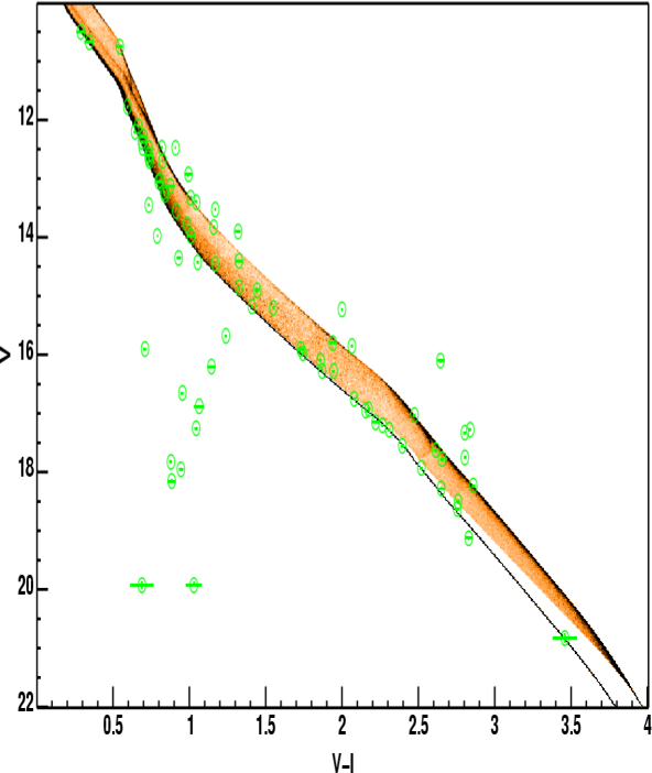
Figure 13: The X-ray selected members of NGC2547 (green circles with error bars) and best fitting model (background image), for a binary fraction of 0.5.

7.5 Changing the binary fraction

Although Figure 13 shows the that the single star sequence is broadly correct, it is harder to assess the fit to the binary stars. The distribution of $\tau^{2}$ for the individual datapoints gives us a useful insight into this. In Section 6.3 we described how we calculate the probability distribution of $\tau^{2}$ for each datapoint before multiplying them together to predict the overall value for $\tau^{2}$ for the fit. Instead of multiplying them, the sum of the probability distributions gives us the expected distribution of $\tau^{2}$ for the datapoints in the best fit. Before carrying out a comparison with the NGC2547 data, we show in Figure 14 the comparison between the actual (histogram) and predicted (curve) distributions of the single-point $\tau^{2}$ values for the simulated cluster used in Section 3. This shows the prediction works very well. In Figure 15 we show the same plot for NGC2547. The real distribution differs from the model in the mid-ranges of $\tau^{2}$, in particular there are more points at $\tau^{2}\simeq 4$ than the model predicts. High values of $\tau^{2}$ correspond to low values of $P_{i}$. The majority of the low values of $P_{i}$ will occur in the region between the single-star and equal-mass-binary sequences, implying that we have underestimated the binary fraction. To test this hypothesis, and to establish whether one must correctly model the binary fraction to determine reliable ages and distances, we re-fitted the data with a binary fraction of 80 percent. The actual and predicted distributions of $\tau^{2}$ shown in Figure 16. Increasing the binary fraction has indeed increased the number of high valued $\tau^{2}$ points, but in fact the model is now systematically lower than the data. Furthermore $P_{r}(\tau^{2})$ is now only 0.14. Clearly a binary fraction of 50 percent is a better fit to the data than 80 percent.

Figure 14: The expected distribution of $\tau^{2}$ (curve) and that obtained from the data (histogram) for the simulated dataset of Section 3.

Figure 15: The expected distribution of $\tau^{2}$ (curve) and that obtained from the data (histogram) for NGC2547, assuming a binary fraction of 50 percent.

Figure 16: The expected distribution of $\tau^{2}$ (curve) and that obtained from the data (histogram) for NGC2547, assuming a binary fraction of 80 percent.

There is a strong temptation at this point to attempt to model the properties of the binaries, and indeed the ability to extract such information is one of our primary motivations for developing $\tau^{2}$. However, it clearly lies outside the scope of this introductory paper to do so. Furthermore, in this case the dataset itself is unsuited to such an experiment. Aside from the question as to whether an X-ray selected sample is biased towards binary stars, the reader should also note that some stars appear above even the equal-mass-binary sequence. Although some of these may be multiple systems with more than two members (which we have ignored in our models), there are three times more of them than we might expect from Duquennoy & Mayor (1991). For the majority of these objects, therefore, our result implies that there is a non-photospheric contribution to their luminosity, which again would not be surprising for an X-ray selected sample, or that we have significant contamination from foreground dwarfs. Either case would clearly preclude a photometric determination of binary parameters. Despite these cautions, it is interesting to note that we obtain a credible value of $P_{r}(\tau^{2})$ for a binary fraction which is close to that determined by Naylor et al. (2002) (60 percent), when they too assumed a flat mass ratio distribution. Equally importantly, with a binary fraction of 80 percent we obtained a distance modulus of 7.82 and an age of 37.5Myr, which is not significantly different from the result for a binary fraction of 50 percent. The conclusion that the binary fraction has little effect on the derived parameters is, in retrospect, unsurprising. It means that the fit is being driven by the single-star sequence, and not being dragged to brighter magnitudes by the binaries.

7.6 Comparison with previous work

Although it is easiest to quote our result in terms of single parameters and their uncertainties, the derived age and distance are strongly correlated. This is summarised in our $\tau^{2}$ space in Figure 17. Interestingly there is a second minimum (not as deep as the primary one) at 53Myr and a distance modulus of 7.63 mags. This is exactly the effect discussed in Section 7.4, and when the fit is examined, we find that the data at bright magnitudes lie systematically above the model.

The age/distance-modulus pair of 25$\pm$5Myr 8.05$\pm$0.10 derived from the $V$/$V-I_{C}$ data in Naylor et al. (2002) clearly lie in the $\tau^{2}$ valley of Figure 17. The position within that valley cannot be directly compared with Naylor et al. (2002) as they used $B$/$B-V$ data to constrain the distance. Perhaps most remarkable is the excellent agreement with the lithium depletion age of Jeffries & Oliveira (2005). The age derived from the lithium depletion boundary depends on the distance modulus. Using the data of Jeffries & Oliveira (2005) and the DAM97 models we derive an age of $37\pm 3$Myr for our best-fit distance modulus of 7.8 mags. However, we can also plot the constraint in Figure 17, which emphasises the concordance between the lithium and isochronal ages. Our error bars in distance just fail to overlap at 1$\sigma$ with those from HIPPARCOS ($8.18^{+0.29}_{-0.26}$) given by Robichon et al. (1999), but the distances are clearly not inconsistent. Our conclusion is, therefore, that when used with real data $\tau^{2}$ fitting gives credible values and uncertainties.

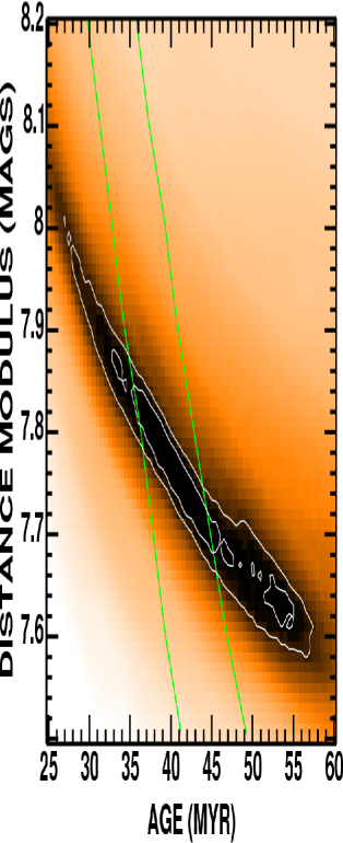
Figure 17: The $\tau^{2}$ grid for fitting the NGC2547 X-ray members to a model with an 80 percent binary fraction. The minimum value of $\tau^{2}$ is 697.8 and the white contours are the 67 percent ($\tau^{2}$=704.6) and 95 percent ($\tau^{2}$=711.8) confidence limits. The observed lithium depletion boundary requires the age and distance to lie between the two green lines.

8 CONCLUSIONS

We have developed a maximum likelihood method for determining parameters for an isochronal population which contains binaries, from its colour-magnitude diagram. We have used numerical simulation to demonstrate it is correct, and used it on a practical example. There is clearly scope for further development. Most obviously one could search many more parameters than we have, determining, for example, binary fraction and mass ratio distribution, mass function, metallicity, or extinction. Several of these could be allowed to vary simultaneously.

One could also use this as a search statistic, looking for populations of a given age in large are surveys. Here the absolute value of $\tau^{2}$ would measure how likely a given “sequence” is to have occurred by chance. Furthermore, one could not only search an N-dimensional colour magnitude space, but might also wish to use other parameters, such as position on the sky modelled against a clustered distribution. Finally there is also a range of other problems to which the technique might be applied such as modelling mass segregation in the mass-radius diagram (e.g. Littlefair et al., 2003), and one could even conceive of a replacement for the 1D Kolmogorov-Smirnov test where the datapoints had associated uncertainties.

References

- Aparicio et al. (1997) Aparicio A., Gallart C., Bertelli G., 1997, AJ, 114, 680
- Borissova et al. (1997) Borissova J., Markov H., Spassova N., 1997, A&AS, 121, 499
- D’Antona & Mazzitelli (1997) D’Antona F., Mazzitelli I., 1997, Memorie della Societa Astronomica Italiana, 68, 807
- Dolphin (1997) Dolphin A., 1997, New Astronomy, 2, 397
- Dolphin (2002) Dolphin A. E., 2002, MNRAS, 332, 91
- Duquennoy & Mayor (1991) Duquennoy A., Mayor M., 1991, A&A, 248, 485
- Durrell & Harris (1993) Durrell P. R., Harris W. E., 1993, AJ, 105, 1420
- Flannery & Johnson (1982) Flannery B. P., Johnson B. C., 1982, ApJ, 263, 166
- Galadi-Enriquez et al. (1998) Galadi-Enriquez D., Jordi C., Trullols E., 1998, A&A, 337, 125
- Georgiev et al. (1999) Georgiev L., Borissova J., Rosado M., Kurtev R., Ivanov G., Koenigsberger G., 1999, A&AS, 134, 21
- Heasley & Christian (1986) Heasley J. N., Christian C. A., 1986, ApJ, 307, 738
- Hertzsprung (1911) Hertzsprung E., 1911, Publikationen des Astrophysikalischen Observatoriums zu Potsdam, 63
- Holland & Harris (1992) Holland S., Harris W. E., 1992, AJ, 103, 131
- Jeffries & Oliveira (2005) Jeffries R. D., Oliveira J. M., 2005, MNRAS, 358, 13
- Jeffries et al. (2001) Jeffries R. D., Thurston M. R., Hambly N. C., 2001, A&A, 375, 863
- Jordi et al. (1996) Jordi C., Trullols E., Galadi-Enriquez D., 1996, A&A, 312, 499
- Jørgensen & Lindegren (2005) Jørgensen B. R., Lindegren L., 2005, A&A, 436, 127
- Littlefair et al. (2003) Littlefair S. P., Naylor T., Jeffries R. D., Devey C. R., Vine S., 2003, MNRAS, 345, 1205
- Mazeh et al. (2003) Mazeh T., Simon M., Prato L., Markus B., Zucker S., 2003, ApJ, 599, 1344
- Naylor & Jeffries (2005) Naylor T., Jeffries R. D., 2005, in Protostars and Planets V, Proceedings of the Conference held October 24-28, 2005, in Hilton Waikoloa Village, Hawai’i. LPI Contribution No. 1286., p.8502 A New Technique for Fitting Colour-Magnitude Diagrams. pp 8502–+
- Naylor et al. (2002) Naylor T., Totten E. J., Jeffries R. D., Pozzo M., Devey C. R., Thompson S. A., 2002, MNRAS, 335, 291
- Nerit et al. (1989) Nerit F., Saittaf G., Chiofalo S., 1989, J. Phys. E: Sci. Instrum., 22, 215
- Noble et al. (1991) Noble R. G., Buttress J., Griffiths W. K., Dickens R. J., Penny A. J., 1991, MNRAS, 250, 314
- Press et al. (1992) Press W. H., Teukolsky S. A., Vetterling W. T., Flannery B. P., 1992, Numerical recipes in FORTRAN. The art of scientific computing. Cambridge: University Press, —c1992, 2nd ed.
- Robichon et al. (1999) Robichon N., Arenou F., Mermilliod J.-C., Turon C., 1999, A&A, 345, 471
- Saha (1995) Saha P., 1995, Principles of Data Analysis. Cappella Archive
- Tolstoy & Saha (1996) Tolstoy E., Saha A., 1996, ApJ, 462, 672
- Trullols & Jordi (1997) Trullols E., Jordi C., 1997, A&A, 324, 549
- von Hippel et al. (2006) von Hippel T., Jefferys W. H., Scott J., Stein N., Winget D. E., DeGennaro S., Dam A., Jeffery E., 2006, ArXiv Astrophysics e-prints
- Wall & Jenkins (2003) Wall J. V., Jenkins C. R., 2003, Practical Statistics for Astronomers. Princeton Series in Astrophysics