Scaling Relations of Dwarf Galaxies without Supernova-Driven Winds

Abstract

Nearby dwarf galaxies exhibit tight correlations between their global stellar and dynamical properties, such as circular velocity, mass-to-light ratio, stellar mass, surface brightness, and metallicity. Such correlations have often been attributed to gas or metal-rich outflows driven by supernova energy feedback to the interstellar medium. We use high-resolution cosmological simulations of high-redshift galaxies with and without energy feedback, as well as analytic modeling, to investigate whether the observed correlations can arise without supernova-driven outflows. We find that the simulated dwarf galaxies exhibit correlations similar to those observed as early as $z\approx 10$, regardless of whether supernova feedback is included. We also show that the correlations can be well reproduced by our analytic model that accounts for realistic gas inflow but assumes no outflows, and star formation rate obeying the Kennicutt-Schmidt law with a critical density threshold. We argue that correlations in simulated galaxies arise due to the increasingly inefficient conversion of gas into stars in low-mass dwarf galaxies rather than supernova-driven outflows. We also show that the decrease of the observed effective yield in low-mass objects, often used as an indicator of gas and metal outflows, can be reasonably reproduced in our simulations without outflows. We show that this trend can arise if a significant fraction of metals in small galaxies is spread to the outer regions of the halo outside the stellar extent via mixing. In this case the effective yield can be significantly underestimated if only metals within the stellar radius are taken into account. Measurements of gas metallicity in the outskirts of gaseous disks of dwarfs would thus provide a key test of such explanation.

1. Introduction

Observational studies of galaxies have revealed the existence of tight correlations between their global stellar and dynamical properties, such as circular velocity, mass-to-light ratio, stellar mass, surface brightness, and metallicity. For example, scalings of the mean metallicity of a galaxy with other global properties such as its luminosity, stellar mass, or total mass, have been established for galaxies of a large range of masses and morphologies (e.g., Lequeux et al., 1979; Garnett & Shields, 1987; Zaritsky et al., 1994; Garnett, 2002; Prada & Burkert, 2002; Dekel & Woo, 2003; Tremonti et al., 2004; Pilyugin et al., 2004; Simon et al., 2006; Lee et al., 2006a). Theoretical modeling of these correlations can help us to identify key physical processes shaping global properties of galaxies.

Supernova energy feedback to the interstellar medium (ISM) with putative associated gas outflows from galaxies has long been a favored mechanism to explain these correlations and other properties of low-mass galaxies (e.g., Larson, 1974; Dekel & Silk, 1986; Arimoto & Yoshii, 1987). The strong effect of the SN feedback on properties of low-mass galaxies is also a standard assumption of the semi-analytic models of galaxy formation (e.g., Lacey et al., 1993; Kauffmann et al., 1993; Cole et al., 1994; Somerville & Primack, 1999; Benson et al., 2003; Croton et al., 2006). Dekel & Woo (2003) argue, for example, that the correlations between circular velocity, stellar mass, metallicity, and stellar surface densities they find for the nearby dwarf galaxies can be reproduced with a simple semi-analytic model incorporating the effect of supernova feedback on the gas component of dwarf galaxies.

The existence of galactic winds has indeed been observationally established in star-forming galaxies at low and high redshifts (e.g., Heckman et al., 2000; Pettini et al., 2001; Martin et al., 2002; Strickland et al., 2004; Martin, 2005; Ott et al., 2005, see Veilleux et al. 2005 for a recent review). An indirect evidence for metal loss in winds is the high-metallicity of the diffuse intergalactic medium in groups and clusters (e.g., Renzini et al., 1993). However, the extent to which the outflows affect the global properties of galaxies and whether the outflow gas escapes the gravitational potential of its host halo or rains back down to the disk remains uncertain. Mac Low & Ferrara (1999) and D’Ercole & Brighenti (1999) used numerical simulations to show that global gas blowout is inefficient in all but the smallest mass halos ($M\lesssim 10^{7}{\rm\ M_{\odot}}$; see also Ferrara & Tolstoy, 2000; Marcolini et al., 2006), although metal-enriched SN ejecta may be removed efficiently. It is also uncertain whether correlations of metallicity with galaxy stellar mass and mass-to-light ratios can be attributed solely to such winds.

In the context of cosmological simulations, the SN feedback is usually ineffective, unless ad hoc phenomenological recipes enhancing SN feedback are employed (e.g., Navarro & White, 1993; Navarro & Steinmetz, 1997; Thacker & Couchman, 2001; Marri & White, 2003; Springel & Hernquist, 2003; Scannapieco et al., 2006). It is likely that this inefficiency is at least partially due to the inability of current cosmological simulations to resolve the scales and processes relevant to stellar feedback. However, it is also possible that the actual effects of feedback on the global properties of galaxies are fairly small in reality. Cosmological simulations at this point cannot make ab initio predictions about the importance or inefficiency of stellar feedback. Observations, on the other hand, although showing evidence for the presence of large-scale winds in actively starforming galaxies (e.g., see Veilleux et al., 2005, for review), are rather uncertain in their estimates of wind mass loss to provide reliable direct observationally-motivated feedback recipes for implementation in simulations. Nevertheless, we can gauge the importance of supernova energy injection by comparing galaxies formed in simulations performed with different assumptions about feedback to observations. In this respect, the smallest dwarf galaxies present the ideal test case because they can be expected to be the most susceptible to the effects of SN feedback due to their shallow potential wells (Larson, 1974; Dekel & Silk, 1986).

The role of feedback in the formation of dwarf galaxies has been investigated in several recent studies. Tassis et al. (2003) used Eulerian AMR simulations of galaxy formation with star formation and SN feedback and found that correlations between mass-to-light ratio and metallicity and stellar mass and metallicity, similar to those observed for the nearby dwarfs, are exhibited by dwarf galaxies in their simulations at $z\gtrsim 3$. The simulations of Tassis et al. (2003) used a rather extreme amount of energy per supernovae to maximize the effects of feedback. They did not test, however, whether feedback or some other mechanism is in fact the dominant factor in shaping the correlations. More recently, Kobayashi et al. (2006) found a tight relation between stellar metallicity and stellar mass at all redshifts in their Smooth Particle Hydrodynamics (SPH) cosmological galaxy formation simulations, which they attributed to the mass-dependent galactic winds. The winds in the model of Kobayashi et al. (2006) do affect the gas and metal content of galaxies significantly, with the effect increasing towards lower mass systems (see their Fig. 16), which plays an important role in shaping the resulting correlation of metallicity and stellar mass.

De Rossi et al. (2006) have recently studied the origin of luminosity- and stellar mass-metallicity relations in cosmological simulations. They find that correlations similar to those observed arise already at high redshifts, although supernova feedback in their simulations is not efficient. This is consistent with our results presented below. Simon et al. (2006) seeked observational correlations between metallicity, surface brightness and mass-to-light ratio within a single galaxy (M33) and found that indeed such correlations exist. They used SPH simulations and analytical calculations to show that feedback is not responsible for these correlations. They found that the presence of feedback decreases the scatter in such relations, although this may at least in part be due to their numerical implementation of feedback. Most recently, Brooks et al. (2006) presented a study of the origin and evolution of the mass-metallicity relation in cosmological simulations. They also concluded that the relation arises not due to the mass loss in winds, but due to increasing inefficiency of star formation in smaller mass galaxies. However, they argue that low effective yields of dwarf galaxies can only be explained by the loss of metals in winds. We argue below that there is an alternative explanation for the low effective yields of dwarfs.

In this paper we investigate the origin of the observed mass-metallicity and other correlations of dwarf galaxies with the specific goal of testing the role of SN feedback. In particular, we discuss results of several high-resolution cosmological simulations of galaxy formation started from the same initial conditions and run with the same prescriptions for star formation and metal enrichment of the ISM, but with different models for gas cooling, UV heating (optically thin approximation vs. self-consistent radiative transfer of the UV radiation), and supernova feedback (see § 4 for details). We follow the simulations until $z\sim 3$.

Although our models simulate galaxies at high redshifts, we study the evolution of the correlations with redshift from $z=9$ to $z\sim 3$ and show that the trends with metallicity and stellar mass are approximately preserved as the galaxy population evolves allowing extrapolation of the results to the present epoch. Therefore, our results and conclusions give us insight to the processes responsible for the properties of observed low-redshift dwarfs. There is indeed observational indication that the stellar mass-metallicity correlation, for example, is already established by $z\sim 1-2$ (Kobulnicky & Kewley, 2004; Savaglio et al., 2005; Erb et al., 2006), although the metallicities of galaxies of a given stellar mass appear to be lower by $\approx 0.3$ dex at $z\sim 2$ compared to $z=0$ (Savaglio et al., 2005; Erb et al., 2006). In addition, for some of the Local Group dwarf galaxies that exhibit these correlations, a significant fraction of their stellar mass was built at $z\gtrsim 3$ (e.g., Dolphin et al., 2005). The correlations for these dwarfs should thus be largely set at high redshifts, which we probe with our simulations.

Our main result is that correlations similar to those observed can be reproduced in all runs, which suggests that supernova energy feedback is not required to explain the observed properties of dwarfs. To interpret the simulation results we use a simple open-box analytic model for the evolution of the baryonic component of dwarf galaxies. We show that a model with gas accretion but no outflows and the Kennicutt law for star formation with the critical density threshold for star formation reproduces the results of our simulations.

This paper is organized as follows. In §2 we summarize the observationally established correlations between global properties of dwarf galaxies that we wish to interpret. Our analytic model and chemical evolution calculations are described in §3. In §4 we describe in detail our cosmological simulations, and in §5 we discuss how global properties of the simulated galaxies are correlated with each other, and we compare these correlations to the observed ones, and to the analytic model of §3. A discussion of observational results on the effective yield and corresponding constraints on the existence of outflows is given in §5.4. We discuss our findings in §6, and we summarize our conclusions in §7.

2. Observed Correlations

Correlations of observables in dwarf galaxies relate the stellar mass, $M_{*}$, with the metallicity $Z$, the surface brightness $\mu_{*}$ and the maximum circular velocity $V_{\rm m}$ of dwarf galaxies. These can be parametrized as the power law relations:

$$Z\propto M_{*}^{n_{Z}}\,;\,\,\,\mu_{*}\propto M_{*}^{n_{\mu}}\,;\,\,\,V_{\rm m}\propto M_{*}^{n_{V}}\,.$$ (1)

The existence of these correlations (in several cases in the form of correlations between absolute magnitudes, rather than stellar masses, and $Z$, $\mu_{*}$ and $V_{\rm m}$) has been established through observations of galaxies with a large range of masses and in a variety of settings, including nearby dwarfs (e.g. Skillman et al., 1989; Dekel & Woo, 2003 based on observations taken from Mateo, 1998,van den Bosch, 2000 and references therein; Lee et al., 2006a; van Zee & Haynes, 2006), dwarf galaxies in the Sloan Digital Sky Survey (SDSS; Tremonti et al., 2004; Kauffmann et al., 2003; Blanton et al., 2003; Bernardi et al., 2003), the Hubble Deep Field (Driver, 1999), the Ursa Major cluster (Bell & de Jong, 2001) and the Virgo cluster (Ferguson & Binggeli, 1994). However, the exact values of the slopes of these relations are affected by systematic uncertainties involved in obtaining stellar masses from the observed quantities (magnitudes). In general, the slopes depend on the the mass range in which they are determined.

For example, in the case of the $Z-M_{*}$ scaling, Dekel & Woo (2003) find that for the Local Group dwarfs in the mass range of $10^{6}{\rm M_{\odot}}\lesssim M_{*}\lesssim 10^{10}{\rm M_{\odot}}$, $n_{Z}\sim 0.4$, while the SDSS data of Tremonti et al. (2004) (see also Gallazzi et al., 2005) indicate that $n_{Z}$ increases with decreasing $M_{*}$: it is quite flat for $M_{*}\gtrsim 3\times 10^{10}{\rm M_{\odot}}$, while it appreciably exceeds the Dekel & Woo (2003) value by $M\sim{\rm few}\times 10^{8}{\rm M_{\odot}}$. Most recently, Lee et al. (2006a) find $n_{Z}\approx 0.29\pm 0.03$ for the dwarf galaxies in their sample.

In the case of the $\mu_{*}-M_{*}$ scaling, Dekel & Woo (2003) find for the Local Group dwarfs the slope of $n_{\mu}\sim 0.55$, although their data points exhibit a scatter around the best-fit line which is large compared to their adopted error bars. For the same scaling, Kauffmann et al. (2003) using SDSS data for the surface density of stellar mass within the half-light radius, find that for a given value of $M_{*}$ there is appreciable scatter (about an order of magnitude) in $\mu_{*}$, and the median value of $\mu_{*}$ scales roughly as $M_{*}^{0.63}$ for $10^{8}\lesssim M_{*}\lesssim 3\times 10^{10}{\rm M_{\odot}}$, and it becomes almost independent of $M_{*}$ for larger $M_{*}$.

In the case of the $M_{*}-V_{\rm m}$ scaling (the Tully-Fisher relation), Bell & de Jong (2001) using galaxies with $3\times 10^{8}{\rm M_{\odot}}\lesssim M_{*}\lesssim 10^{11}{\rm M_{\odot}}$ find $n_{V}\sim 0.21-0.24$, and a shallower correlation with baryonic mass (i.e. stars plus gas), $n_{V}\sim 0.27-0.30$. Several recent studies also find that the $V_{\rm m}-M_{*}$ relation for low-mass galaxies ($V_{\rm m}\lesssim 90$ km/s) is steeper and exhibits considerably more scatter than the baryonic Tully-Fisher relation of the same galaxies (Matthews et al., 1998; McGaugh et al., 2000; Bell & de Jong, 2001; Gurovich et al., 2004; McGaugh, 2005; Geha et al., 2006). These studies find slopes of $n_{V}\approx 0.1-0.2$ for the $M_{*}-V_{\rm m}$ relation of the dwarf galaxies (McGaugh et al., 2000; Gurovich et al., 2004) and $n_{V}\approx 0.25-0.33$ for the baryonic $M_{\rm baryon}-V_{\rm m}$ relation (e.g., McGaugh et al., 2000; Verheijen, 2001; Bell & de Jong, 2001; McGaugh, 2005; Geha et al., 2006). For the Local Group dwarfs, Dekel & Woo (2003) obtain $n_{V}\sim 0.37$ for $10^{8}{\rm M_{\odot}}\lesssim M_{*}\lesssim 10^{10}{\rm M_{\odot}}$ and $n_{V}\sim 0$ for $10^{6}{\rm M_{\odot}}\lesssim M_{*}\lesssim 10^{8}{\rm M_{\odot}}$.

Finally, another tight relation found in Local Group dwarf galaxies is the correlation between the dynamical mass-to-light ratio and average metallicity (Prada & Burkert, 2002):

$$\log(M_{\rm dyn}/L_{V})\propto-{\rm[Fe/H]}\,.$$ (2)

3. Analytical Model for the Evolution of the Baryonic Component of Dwarf Galaxies

In this section we present a simple analytic model for the evolution of the baryonic component (gas, stars and metals) of dwarf galaxies at high redshifts, which we will make to interpret our simulation results. The model is based on the following assumptions:

(1) Galaxies accrete gas at a rate consistent with simulations, but no gas or metals escape outside the virial radius of the parent halo.

(2) The gas mass of each galaxy is proportional to its total (dynamical) mass, $M_{\rm gas}\propto M$. At early epochs $M_{*}\ll M_{\rm gas}$, which implies for the baryonic mass $M_{\rm b}=M_{\rm gas}+M_{*}\approx M_{\rm gas}$. The gas fraction within halos in our simulations is approximately independent of the total (dynamical) mass for $M_{\rm tot}\gtrsim 10^{9}{\rm M_{\odot}}$ (see §5, Fig. 2), which is consistent with the results of independent simulations of Tassis et al. (2003). Therefore this assumption is an excellent approximation for all but the smallest objects in the simulation, which are excluded in our analysis of other global quantities. Although at lower redshifts the total baryon fraction in small mass galaxies $M<10^{10}\ M_{\odot}$ can be suppressed due to heating by the cosmic UV background (e.g., Gnedin, 2000; Hoeft et al., 2006), our results would still be applicable to galaxies in which a significant fraction of stars is formed at high redshifts before such suppression has occurred in the mass range we consider. We should stress that we intend to apply our model only to such stellar populations.

(3) The gas in galaxies forms an exponential disk with radial extent proportional to the virial radius of the parent halo. The disk is assumed to be more extended and consequently less compressed for smaller objects with $T_{\rm vir}<10^{4}$ K, in which gas cannot cool efficiently.

(4) Gas is converted into stars at a rate given by the Kennicutt law of star formation with a density threshold (e.g., Martin & Kennicutt, 2001). Gas at densities below the threshold does not form stars. Note that the Kennicutt law with the threshold is reproduced by our numerical simulations, but it is not assumed a priori. The numerical simulations implement a much simpler recipe for star formation (see §4).

(5) Instantaneous recycling approximation: i.e., no time delay is assumed between the birth of a generation of stars and the corresponding metal enrichment of the ISM. Hence, we implicitly assume that the metal enrichment due to type II supernovae is dominant. This is appropriate for all but the most massive dwarf galaxies.

The key ingredient of our model is the relation between the gas mass and the stellar mass of a galaxy. We will first derive this correlation, and subsequently use it to derive relations between the stellar mass, gas mass, stellar surface density, metallicity, and circular velocity of high-$z$ galaxies.

3.1. Stellar Mass - Gas Mass Relation

The relation between stellar mass and total gas mass in dwarf galaxies is central to understanding the origin of correlations between other observable quantities. In this section, we derive such a relation. In subsequent sections, we will use it to explain the correlations discussed in §2 and we will directly compare it against our simulation results.

The rate of change of the gas mass, assuming that there are no significant gas outflows due to SN-driven winds, is

$$\frac{d}{dt}(M_{\rm gas})=F-a\psi\,,$$ (3)

where $F$ is the gas mass accretion rate, $\psi$ is the star formation rate, and $a$ is the fraction of stellar mass locked in long-lived stars and remnants (i.e., not returned to the ISM). The rate of change of the stellar mass is

$$\frac{dM_{*}}{dt}=a\psi\,.$$ (4)

If the dependence of $\psi$ and $F$ on $M_{\rm gas}$, as well as any explicit dependence on redshift, are known, then equations (3) and (4) can be integrated in time as a system of two ordinary differential equations. Different initial conditions for $M_{\rm gas}$ at some early time (for which we can safely assume that $M_{*}=0$) will produce different pairs of $(M_{\rm gas},M_{*})$ at any time of interest. In this way, we calculate parametrically the prediction of our analytic model for the $M_{*}-M_{\rm gas}$ relation.

As we show in the Appendix, $F$ is proportional to the gas mass and $\psi$ depends on the extent of the gaseous disk (which in turn depends on the dynamical mass of the galaxy and the angular momentum parameter, $\lambda$) and the star formation density threshold, $\Sigma_{\rm th}$.

Figure 1.— Sensitivity of the analytic model to the angular momentum parameter $\lambda$ and the surface density threshold for star formation, $\Sigma_{\rm th}$, at $z=4$. Solid line: fiducial model with $\lambda=0.033$ (its most probable value) and $\Sigma_{\rm th}=5\,{\rm M_{\odot}}{\,\rm pc^{-2}}$. Dashed lines: model results for $\Sigma_{\rm th}=5\,{\rm M_{\odot}}{\,\rm pc^{-2}}$ and $\lambda=0.023$ (left dashed line) or $\lambda=0.044$ (right dashed line). Dotted lines: model results for $\lambda=0.033$ and $\Sigma_{\rm th}=2\,{\rm M_{\odot}}{\,\rm pc^{-2}}$ (left dotted line) or $\Sigma_{\rm th}=10\,{\rm M_{\odot}}{\,\rm pc^{-2}}$ (right dotted line).

The free parameters which control the normalization and the shape of the $M_{\rm gas}-M_{*}$ relation are $\lambda$ and $\Sigma_{\rm th}$. The solution of Eqs. (3) and (4) for the fiducial values of these parameters is plotted with the solid line in Fig. 1. At high gas masses, $M_{*}$ has a power-law dependence on $M_{\rm gas}$, with a slope set by the slope of the star-formation law. At lower $M_{\rm gas}$, this relation exhibits a break, which is a result of the threshold in the star-formation law resulting in very inefficient star formation at the low densities achieved by inefficiently cooling low-mass galaxies.

Remarkably, we find that the best fit to our data at $z=4$ is obtained when both free parameters have their fiducial values, $\lambda=0.033$ (the most probable value) and $\Sigma_{\rm th}=5\,{\rm M_{\odot}}{\,\rm pc^{-2}}$ (the “canonical” observational value). Figure 1 shows the sensitivity of our analytic model to the values of $\lambda$ and $\Sigma_{\rm th}$. The solid line represents the $z=4$ model results for the fiducial parameter values (which are also the best-fit parameters). The dashed lines show the range of $\lambda$ values that brackets the scatter of our simulation data points at $z=4$. The range of $\lambda$ values represented here is $0.023\lesssim\lambda\lesssim 0.044$ (which contains $\sim 40\%$ of the area under the $\lambda-$probability distribution, and is centered around the distribution peak). In this case, $\Sigma_{\rm th}$ is kept at its fiducial value. The dotted lines show the range of $\Sigma_{\rm th}$ values that brackets the scatter of our data. The range of $\Sigma_{\rm th}$ values represented here is $2\,{\rm M_{\odot}}\,{\rm pc^{-2}}\lesssim\Sigma_{\rm th}\lesssim 10\,{\rm M_{\odot}}\,{\rm pc^{-2}}$. In this case, $\lambda$ is kept at its fiducial value. The asymptotic slope of the curve at higher masses, remains largely independent of parameter choice.

3.2. Mass-to-light ratio vs. metallicity

Under the assumptions of negligible inflow or outflow of metals and instantaneous recycling, and for a fixed initial mass function, the mass of metals of low-$Z$, high-$z$ galaxies is proportional to the stellar mass. From $M_{\rm Z}=ZM_{\rm gas}\propto M_{*}$ we can immediately write

$$Z\propto\frac{M_{*}}{M_{\rm gas}}\,.$$ (5)

Assumption (2), $M_{\rm gas}\propto M$, then gives $Z\propto M_{*}/M$. The luminosity of an object, $L$, can be considered proportional to its stellar mass. Then, Eq. (5) becomes $Z\propto L/M$ or

$$M/L\propto Z^{-1},$$ (6)

in agreement with observations and, as shown in §5, the results of our simulations. This is a simple interpretation of the correlation between the mass-to-light ratio and metallicity found by Prada & Burkert (2002).

3.3. Additional Correlations

We can use the $M_{\rm gas}-M_{*}$ relation we derived in §3.1 in combination with Eq. (5) and assumptions $M_{\rm gas}\propto M$ and $L\propto M_{*}$ to derive additional relations between stellar mass and stellar surface density, metallicity, and circular velocity of high-$z$ galaxies. We will overplot these relations with our simulation results and discuss them in §5.

4. Numerical Simulations

Table 1Simulations

Simulation	SN energy feedback	cooling	3-D rad. transfer
FEC	yes	equilibrium	no
NFEC	no	equilibrium	no
FNEC-RT	yes	non-equilibrium	yes
F2NEC-RT	yes	non-equilibrium	yes

In this study we use four simulations (Table 1) of the early ($z\gtrsim 3$) stages of evolution for a Lagrangian region of a MW-sized system of total (dark matter and baryons) virial mass $\approx 10^{12}h^{-1}\ \rm M_{\odot}$ at $z=0$. The simulations were performed using the Eulerian, gasdynamics $+N$-body Adaptive Refinement Tree (ART) code (Kravtsov et al., 1997; Kravtsov, 1999). In both the gasdynamics and gravity calculations, a large dynamic range is achieved through the use of adaptive mesh refinement (AMR). At the analyzed epochs, the galaxy has already built up a significant portion of its final total mass: $1.3\times 10^{10}h^{-1}\ \rm M_{\odot}$ at $z=9$ and $2\times 10^{11}h^{-1}\ \rm M_{\odot}$ at $z=4$. The evolution is started from a random realization of a gaussian density field at $z=50$ in a periodic box of $6h^{-1}\ \rm Mpc$ with an appropriate power spectrum and is followed assuming flat $\Lambda$CDM model: $\Omega_{0}=1-\Omega_{\Lambda}=0.3$, $\Omega_{b}=0.043$, $h=H_{0}/100=0.7$, $n_{s}=1$, and $\sigma_{8}=0.9$.

To achieve the high mass resolution, a low-resolution simulation was run first and a galactic-mass halo was selected. A Lagrangian region corresponding to five virial radii of the object at $z=0$, corresponding to a region of $\sim 3h^{-1}$  comoving Mpc in diameter, was then identified at $z=50$ and re-sampled with additional small-scale waves (Navarro & White, 1994, the specific procedure described here is described in Klypin et al. 2001). The total number of DM particles in the high-resolution Lagrangian region is $2.64\times 10^{6}$ and their mass is $m_{\rm DM}=9.18\times 10^{5}h^{-1}\ \rm M_{\odot}$. In addition to the main progenitor of the MW-sized system this Lagrangian region contains several dozens of smaller galaxies spanning a wide range of masses. We will use these galaxies to analyze correlations between their properties.

The code used a uniform $64^{3}$ grid to cover the entire computational box. The Lagrangian region, however, was always unconditionally refined to the third refinement level, corresponding to the effective grid size of $512^{3}$. As the matter distribution evolves, the code adaptively and recursively refines the mesh in high-density regions beyond the third level using two refinement criteria: gas and DM mass in each cell. A mesh cell was tagged for refinement if its gas or DM mass exceeded $1.2\times 10^{6}h^{-1}\ \rm M_{\odot}$ and $3.7\times 10^{6}h^{-1}\ \rm M_{\odot}$, respectively. The maximum allowed refinement level was $l_{\rm max}=9$. The volume of high-density cold star forming disks forming in DM halos was refined to $l_{\rm max}=9$. The physical size of mesh cells in the simulations was $\Delta x_{l}=26.16\,\,[10/(1+z)]2^{9-l}\ \rm pc$, where $l$ is the cell’s level of refinement. Each refinement level was integrated with its own time step $\Delta t_{l}=\Delta t_{0}2^{-l}\approx 2\times 10^{4}\,\,2^{9-l}\ \rm yrs$. The time steps are set by a global Courant-Friedrich-Levy condition.

The analyzed simulations were started from the same initial conditions, but evolved using different assumptions about cooling and heating processes accompanying galaxy formation. All four runs include star formation using the recipe described in Kravtsov (2003). Namely, the gas is converted into stars on a characteristic gas consumption time scale, $\tau_{\ast}$: $\dot{\rho}_{\ast}=\rho_{\rm g}/\tau_{\ast}$. We use constant, density-independent $\tau_{\ast}$. This is different from the commonly used density-dependent efficiency, but may be more appropriate for star forming regions on $\sim 100$ pc scales which are resolved in the simulations where constant star formation efficiency is indicated by observations (e.g., Young et al., 1996; Wong & Blitz, 2002). As shown by Kravtsov (2003), such constant efficiency assumption at the scales of molecular clouds results in the Kennicutt-like star formation law on kiloparsec scales, although a Kennicutt law is not a priori assumed. The star formation was allowed to take place only in the densest cold regions, $\rho_{\rm g}>\rho_{\rm SF}$ and $T_{\rm g}<T_{\rm SF}$, but no other criteria (like the collapse condition $\nabla\cdot{\bf v}<0$) were imposed. We used $\tau_{\ast}=4$ Gyrs, $T_{\rm SF}=10^{4}$ K, and $\rho_{\rm SF}=1.64{\ \rm M_{\odot}pc^{-3}}$ corresponding to atomic hydrogen number density of $n_{\rm H,SF}=50{\ \rm cm^{-3}}$.

Our fiducial simulation (FEC) includes metallicity-dependent cooling and UV heating due to cosmological ionizing background with equilibrium cooling and heating rates tabulated for the temperature range $10^{2}<T<10^{9}$ K using the Cloudy code (ver. 96b4, Ferland et al., 1998). The cooling and heating rates take into account Compton heating/cooling of plasma, UV heating, atomic and molecular cooling. It also includes energy feedback and chemical enrichment due to supernovae assuming the Miller & Scalo (1979) stellar initial mass function (IMF) and stellar masses in the range $0.1-100\ \rm M_{\odot}$. All stars with $M_{\ast}>8{\ \rm M_{\odot}}$ deposit $2\times 10^{51}$ ergs of thermal energy and a mass $f_{\rm Z}M_{\ast}$ of heavy elements in their parent cell (no delay of cooling was introduced in these cells). The metal fraction is $f_{\rm Z}={\rm min}(0.2,0.01M_{\ast}-0.06)$, which crudely approximates the results of Woosley & Weaver (1995).

The second simulation, NFEC, is identical to the FEC run in all respects, except that it did not include the energy injection due to SNe (chemical enrichment due to SNe is still included). Note that the cooling rates in the run with feedback accounted for the local metallicity of the gas, while in the run with no feedback the significantly lower zero-metallicity cooling rates were used.

The third simulation, FNEC-RT, includes star formation and SN enrichment and energy feedback in the same way as the FEC run, but uses self-consistent 3-D radiative transfer of UV radiation from individual stellar particles using the OTVET algorithm (Gnedin & Abel, 2001; Iliev et al., 2006) and follows non-equilibrium chemical network of hydrogen and helium species (the details of the specific implementation of the OTVET algorithm on adaptively refined meshes will be described elsewhere). The simulation thus includes non-equilibrium cooling and heating rates which make use of the local abundance of atomic, molecular, and ionic species and UV intensity followed self-consistently during the course of the simulation. The metallicity-dependence of cooling rates is taken into account using optically thin equilibrium metal cooling functions from Sutherland & Dopita (1993) in the high metallicity regime and from Penston (1970) and Dalgarno & McCray (1972) in the low metallicity regime. The molecular hydrogen formation on dust is taken into account using Cazaux & Spaans (2004) rates, and gas cooling on dust is based on Draine (1981).

A severe limitation of our current treatment of molecular hydrogen formation is that self-shielding of molecular lines in the Lyman-Werner band is not taken into account, which results in a substantial underestimate of the molecular fractions at the high density regime ($n\gtrsim 100{\rm\,cm}^{-3}$). Note, however, that since our star formation criterion is based on the total rather than molecular gas density, this does not affect our star formation rates significantly.

Finally, the fourth simulation, F2NEC-RT, is identical to the FNEC-RT but SN energy is injected with a delay of $10^{7}$ years after the star forming event and energy release is spread over $10^{7}$ years after that. This variation is intended to test the sensitivity of our results to the specific details of the feedback implementation. Energy injection with delay was argued to enhance the efficiency and impact of the SN feedback on the ISM (Slyz et al., 2005), as the stellar particles have time to leave the densest regions where they form and release their energy at lower densities where the cooling time is longer. This change of feedback recipe results in a significant enhancement of the star formation efficiency. Perhaps surprisingly, the F2NEC-RT simulation forms nearly twice as much stellar mass as the simulation FNEC-RT. The reason is simple. With a delayed energy release the star forming regions are generally left intact and continuing forming stars in the simulation F2NEC-RT, while in the FNEC-RT the temperature of gas in star forming regions is increased due to SN feedback and star formation ceases for some period of time.

We show below that the details of the specific implementation of feedback in our simulations do not affect the correlations of galaxy properties and our conclusions.

5. Results

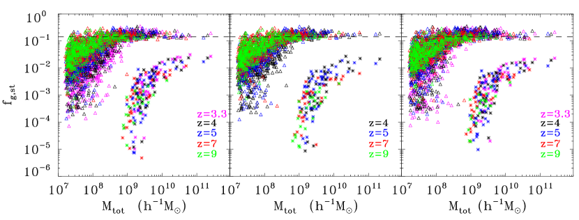
Figure 2.— Gas and stellar mass fractions of objects in our simulations plotted against the total (dark matter + total baryonic) mass of each object. Left panel: simulation FEC; middle panel: simulation NFEC; right panel: simulation FNEC-RT. Open triangles show the gas fraction ($M_{\rm gas}/M_{\rm tot}$), while stars show the star fraction $M_{*}/M_{\rm tot}$. Different colors correspond to different redshifts as detailed in the legend. The horizontal dashed line corresponds to the baryonic mass fraction ($\Omega_{\rm b}/\Omega_{0}=0.14$)

In this section, we discuss relations between global properties of galaxies in our cosmological simulations, how these depend on the detailed physics included in each simulation, and how they compare to the observationally established correlations and our analytic models of §3.

The panels in the figures discussed in this section are arranged in the following way: left panel - FEC simulation (SN feedback, uniform UV background, tabulated heating/cooling rates); middle panel - NFEC simulation (no SN energy feedback, uniform UV background, tabulated heating/cooling rates); right panel - FNEC-RT simulation (SN feedback, 3-D radiative transfer). We do not show the results of the F2NEC-RT simulations in all of the figures for clarity. In all cases, the results of the F2NEC-RT simulations are quite similar to those of the FNEC-RT run.

5.1. Baryonic Content of Simulated Galaxies

Figure 3.— Star-to-baryonic mass ratio vs. gas mass for objects in each of the analyzed simulations. The gas mass here is the total gas in each halo. Left panel: simulation FEC; middle panel: simulation NFEC. Right panel: the FNEC-RT simulation. Different symbols correspond to different redshifts as detailed in the legend. The solid and dashed lines show the results of our analytic model for $z=4$ and $z=9$, respectively.

Figure 2 shows the gas and stellar mass fractions (total gas mass over total dynamical mass, and stellar mass mass over total dynamical mass, respectively) within the virial radius as a function of the virial mass for all objects in the simulations. For systems with $M\gtrsim 10^{9}\,{\rm M_{\odot}}$, the gas fractions are approximately independent of mass, while at smaller masses a variety of effects (e.g., gas stripping, reionization) act to suppress the gas fractions and increase the scatter. This result is qualitatively consistent with the findings of the previous studies (e.g., Gnedin, 2000; Chiu et al., 2001; Tassis et al., 2003; Hoeft et al., 2006). Figure 2 also shows that the stellar fractions for the redshifts and masses under consideration is an order of magnitude smaller than the gas fractions. This is due both to the inefficiency of star formation in these small systems and the fact that we analyze them at high redshifts, where they did not have the sufficient amount of time to convert their gas into stars. Most interestingly, the stellar fractions drop sharply in systems with $M\lesssim 5\times 10^{9}\rm\,M_{\odot}$. The objects with smaller masses do contain a universal share of the baryons in the form of gas, but fail to convert a sizeable fraction of it into stars. Note that all three simulations shown produced very similar results. This demonstrates explicitly that the inefficiency of star formation at small masses is not due to SN feedback. We note however that objects in these small-mass systems are resolved with just a few thousand DM particles. Convergence tests with much higher resolution simulations are therefore needed to test whether inefficient star formation at the smallest masses is not a numerical artefact.

Figure 4.— Gas metallicity vs. stellar metallicity. Left panel: simulation FEC; middle panel: simulation NFEC; right panel: FNEC-RT simulation. Different symbols correspond to different redshifts as detailed in the legend. The solid line corresponds to $Z_{\rm gas}=Z_{*}$.

Figure 3 shows the star-to-baryonic mass ratio of the simulated galaxies plotted against their gas mass. A tight correlation between the two quantities exists, although it cannot be described by a single power law for the entire range of masses examined here. At the high-mass end, $M_{\rm g}\gtrsim 10^{9}\,{\rm M_{\odot}}$, the stellar mass is roughly proportional to the baryonic mass (and hence, in the gas-rich regime, to the gas mass). At lower masses, however, the relation exhibits a break and becomes considerably steeper as the stellar mass of low-mass objects is suppressed (see also Chiu et al., 2001). This correlation is central in identifying the origin of the scalings between the rest of the global properties we present below. The solid and dashed lines represent the prediction of the model discussed in § 3, for redshifts $z=4$ and $z=9$, respectively. The agreement with the simulation data is excellent. Here again we see that the results of the three different simulations are consistent with each other.

5.2. Correlations Involving Metallicities

Figure 5.— Ratio between total mass and stellar mass (assumed to be proportional to the mass-to-light ratio of each object), plotted against stellar metallicity. Left panel: simulation FEC; middle panel: simulation NFEC; right panel: FNEC-RT simulation. Different symbols correspond to different redshifts as detailed in the legend. The solid line corresponds to the $M_{\rm tot}/M_{*}\propto Z^{-1}$ scaling

.

Figure 6.— Stellar metallicity as a function of stellar mass. Left panel: simulation FEC; middle panel: simulation NFEC; right panel: FNEC-RT simulation. Different symbols correspond to different redshifts as detailed in the legend. The solid and dashed lines show the results of our analytic model for $z=4$ and $z=9$, respectively.

Before we proceed to discuss the correlation of the metallicities in the simulated galaxies with other observables, we should make a note about the distinction between stellar and gas metallicities. Metallicities in stars represent an average metallicity over the star formation history of the observed object, while gas metallicities are actually representative of the amount of metals currently present in the interstellar medium. Observationally, either one or both can be measured and used. For example, Dekel & Woo (2003) use stellar metallicities for dE galaxies and gas oxygen abundance for dIrr, while Prada & Burkert (2002) use stellar metallicities in all cases. The metallicity in the gas and in the stars, although not the same in general, are related to each other. This is particularly true for the high-redshift galaxies in our simulations. Figure 4 shows the metallicity in the gas versus the metallicity in stars for every object in our simulations at different redshifts. The solid line corresponds to the one-to-one relation $Z_{\rm gas}=Z_{*}$. Indeed, for the objects and redshifts we consider, the metallicity of stars tracks that of the gas very closely.

A tight correlation observed for the nearby dwarf galaxies is the correlation of the dynamical mass-to-light ratio and metallicity (Prada & Burkert, 2002). In § 3.2 we showed that such a correlation should naturally arise in low-metallicity dwarf galaxies without gas outflows and regardless of their star formation rate as long as their baryon mass is approximately proportional to their total mass. Figure 5 clearly shows that for galaxies in our simulations the ratio of the total (baryonic + dark matter) to stellar mass is tightly correlated with metallicity, independently of the details of star formation and cooling and inclusion of SN feedback. The form of the correlation, $M/M_{*}\propto Z^{-1}$ is similar to that exhibited by the observed dwarf galaxies. The correlation arises for objects at the earliest epochs, which implies that a similar correlation should be expected to hold for the observed galaxies at high redshifts.

Basic assumptions in the derivation of this correlation is that $M_{\rm gas}\propto M$ and $Z\ll Z_{\odot}$, implying that at the time this correlation is being established, the galaxy is in the gas-rich, low-metallicity regime. For galaxies in which star formation is inefficient and which have not lost substantial amount of gas (due to, e.g., ram or tidal stripping), it is clear that both assumptions are likely to hold until late times. Such galaxies may move along the correlation as they evolve, but they will remain on the same line. However, such galaxies are not the only objects which may retain this correlation until the current cosmic epoch: in galaxies where star formation is halted early on (when our derivation assumptions are still valid) and gas is stripped from them, neither the metallicity nor the dark matter or the stellar mass of the galaxy would be affected. Hence the correlation between $M/M_{*}$ and $Z$ would be preserved. This would then be a typical example of a “fossil” correlation, established in the early phases of the evolution of a galaxy and preserved until the present cosmic epoch due to lack of additional evolution of the observable quantities involved.

Figure 6 shows the mass-weighted metallicity of stars of the simulated galaxies as a function of stellar mass. The correlation of the two quantities is very tight and can be described by a power law at small masses. At large stellar masses, $M_{*}\gtrsim 5\times 10^{8}\,{\rm M_{\odot}}$, the correlation becomes shallower. This is qualitatively consistent with the flattening of the $Z-M_{*}$ relation found in the SDSS data (Tremonti et al., 2004), although in their observations the break occurs at much larger masses: $m\sim 3\times 10^{10}\,{\rm M_{\odot}}$. Note, however, that this figure should not be directly compared to the present-day correlation over a wide range of stellar masses because massive galaxies will undergo substantial evolution in both their stellar mass and metallicity between $z=3$ and the present, while the evolution of dwarf galaxies is expected to be much slower. For some of the dwarf galaxies the evolution can be halted at high redshifts if their gas is removed by some process (e.g., ram pressure stripping). Thus, the comparison with the correlations exhibited by the local galaxies is most meaningful for smaller mass objects.

The solid lines in Figure 6 show the results of our analytic model. The model reproduces the slope of the correlation in the two mass regimes, the location of the break, and the observed redshift evolution seen in the simulated galaxies. The correlation in the model arises mainly due to the inefficiency of star formation in dwarf galaxies and the existence of star formation threshold, without gas outflows. Interestingly, direct extrapolation of the model to $z=0$ indicates that the flattening of the $M_{*}-Z$ relation shifts to $M_{*}\sim{\rm few}\times 10^{10}\,{\rm M_{\odot}}$, in agreement with the SDSS data. However, the reader should keep in mind that certain assumptions ($Z\ll Z_{\odot}$, $M_{*}\ll M_{\rm gas}$) of our analytic model are expected to eventually break down at late times (especially for the higher-mass objects), and hence additional effects may become important in shaping the present-day properties of higher-mass galaxies.

5.3. Correlations Involving Stellar and Total Masses

Figure 7.— Stellar mass within $R_{*}$ over $R_{*}^{2}$ (where $R_{*}$ is the half-light radius, which includes $50\%$ of the stellar mass of each object), plotted against stellar mass. Left panel: simulation FEC; middle panel: simulation NFEC; right panel: FNEC-RT simulation. Different symbols correspond to different redshifts as detailed in the legend. The solid line corresponds to the prediction of out analytic model for $z=4$.

Figure 7 shows the stellar surface density, $\mu_{*}$, against galaxy stellar mass. The surface density is calculated from the simulation data as $\mu_{*}\propto M_{*}/R_{*}^{2}$, where $R_{*}$ is the half-light radius, defined as the radius which includes $50\%$ of the stellar mass. The data occupy a primary locus in the $\mu_{*}-M_{*}$ plane, which is traced by the prediction of our analytic model, in which stellar surface density is calculated as $\mu\propto M_{*}/r_{\rm th}^{2}$. At masses $M_{*}\lesssim 10^{8}\,{\rm M_{\odot}}$ there are several outliers, as in this regime star formation becomes more stochastic. As for the other considered correlations, we see that the results of different simulations are consistent, although the NFEC and FNEC-RT simulations do show a higher $\mu_{*}$ for comparable $M_{*}$ at the high-$M_{*}$ end, an indication that in these simulations the stellar populations appear to be more concentrated. We should note however that stellar surface densities are probably less reliable than global properties, such as stellar mass, because they depend on the internal structure of the stellar distribution in galaxies and may be more susceptible to resolution effects.

Figure 8 shows the stellar mass of the objects in our simulations as a function of their maximum rotational velocity (the Tully-Fisher relation). A break of the scaling law exists at a stellar mass of $\sim 10^{8}\,{\rm M_{\odot}}$. For objects with stellar masses above the break, the stellar mass scales as $V_{\rm m}^{\alpha}$ with the best fit slopes of $3.41\pm 0.33$, $3.34\pm 0.33$, and $3.37\pm 0.22$ for the FEC, NFEC, and FNEC-RT simulations. Below the break the $V_{\rm m}-M_{*}$ relation steepens considerably. The location of objects on the $M_{*}-V_{\rm m}$ plane exhibits a considerable shift with redshift. This is a trivial consequence of the redshift-dependence of the virial density.

Figure 8.— Maximum circular velocity as a function of stellar mass (Tully-Fisher relation). Left panel: simulation FEC; middle panel: simulation NFEC; right panel: FNEC-RT simulation. Different symbols correspond to different redshifts as detailed in the legend. The solid and dashed lines show the results of our analytic model for $z=4$ and $z=9$, respectively. In the lower row plots we have shifted $V_{\rm m}$ by a factor of $(1+z)^{-0.5}$ to correct for the explicit redshift dependence entering $V_{\rm m}$ through its dependence on the virial radius.

From the virial theorem we have

$$V_{\rm m}\propto\sqrt{M/R_{\rm vir}}\,.$$ (7)

At the high redshifts under consideration, the universe is matter-dominated, and the virial overdensity $\delta_{\rm vir}=\rho_{\rm vir}/\rho_{\rm m}-1\approx 18\pi^{2}$ is essentially independent of $z$. The virial radius is then determined from the relation

$$\frac{4}{3}\pi R_{\rm vir}^{3}\rho_{\rm m}(z)(1+\delta_{\rm vir})=M\,.$$ (8)

Given that $\rho_{\rm m}(z)=\rho_{\rm m,0}(1+z)^{3}$, we get

$$R_{\rm vir}\propto\frac{M^{1/3}}{1+z}\,.$$ (9)

and hence

$$V_{\rm m}\propto M^{1/3}\sqrt{1+z}\,.$$ (10)

In the lower panels of Figure 8, we have scaled the $V_{\rm m}$ values of all data points of the upper panel by $\sqrt{1+z}$ to correct for this redshift evolution. Using $M\propto M_{\rm gas}$ and the $M_{*}=M_{*}(M_{\rm gas})$ dependence calculated using our analytic model, we get the solid and dashed lines shown in Figure 8, for $z=4$ and $z=9$, respectively. Once again, the model describes the results of the simulation very well.

Finally, Figure 9 shows the baryonic Tully-Fisher relation, where the total baryonic mass (stars and gas) of each object is plotted against $V_{\rm m}$. In this case, the $M_{\rm baryon}\propto V_{\rm m}^{3}$ scaling (represented by the solid line) shows no evidence of a break. This is similar to the behavior of the observed dwarfs, which exhibit a break in the $M_{*}-V_{\rm m}$ relation, but a tight power law $M_{\rm b}-V_{\rm m}$ relation (see § 2).

Figure 9.— Maximum circular velocity as a function of baryonic mass (baryonic Tully-Fisher relation). Left panel: simulation FEC; middle panel: simulation NFEC; right panel: FNEC-RT simulation. Different symbols correspond to different redshifts as detailed in the legend. The solid line corresponds to the $M_{\rm baryon}\propto V_{\rm m}^{3}$ scaling. In the lower row plots we have shifted $V_{\rm m}$ by a factor of $(1+z)^{-0.5}$ to correct for the explicit redshift dependence entering $V_{\rm m}$ through its dependence on the virial radius.

5.4. The Effective Yield

Figure 10.— Effective yield as a function of circular velocity of galaxies in our simulations at $z=4$. Left column: simulation FEC (with supernova energy feedback); right column: simulation NFEC (no supernova energy feedback). Upper panel: effective yield $y_{\rm eff}^{\rm tot}$ calculated taking into account the mass of gas, stars, and metals within the virial radius of each object; lower panel: effective yield $y_{\rm eff}^{\rm obs}$ calculated using the metallicity of the stellar disk and the gas fraction calculated using all cold gas within the halo.

The effective yield, defined as

$$y_{\rm eff}=\frac{Z}{\ln(1/f_{\rm g})},$$ (11)

has been widely used as a diagnostic of the evolution of the baryonic component of galaxies, and more specifically as a “litmus test” of the validity of the closed-box approximation. Here, $f_{\rm g}=M_{\rm gas}/(M_{*}+M_{\rm gas})$ is the fraction of baryons in the gas phase. Under the closed-box assumption, the effective yield is always equal to the true yield $y_{\rm true}$, defined as the mass in newly synthesized metals returned to the ISM by a stellar population normalized to the stellar mass of this population locked-up in stellar remnants and long-lived stars.

Edmunds (1990) showed that $y_{\rm eff}$ cannot exceed $y_{\rm true}$. Values of $y_{\rm eff}$ lower than $y_{\rm true}$ are indicative of the deviations from the closed-box model due to either inflows or outflows of gas and metals. Observationally, dwarf galaxies ($V_{\rm m}\lesssim 100{\rm\,km/s}$) have low values of $y_{\rm eff}$. This has been interpreted as strong evidence for significant outflows of metals and/or gas, which can reduce the metallicity and/or the gas fraction and are expected to be more prevalent in smaller objects with shallower gravitational potentials (Garnett, 2002; Tremonti et al., 2004; Pilyugin et al., 2004).

In the previous section we showed that global correlations of galaxy properties arise in our simulations without SN-driven outflows. We have shown that these correlations can be reproduced with an open-box evolution with cosmological mass inflow but no outflows and 1) mass-dependent gas distribution given by equation (B3) and 2) star formation obeying the Kennicutt law with a surface density threshold. In this model the correlations, similar to those of observed galaxies, arise due to the increasing fraction of gas at surface densities below the star formation threshold density (and, correspondingly, inefficiency of star formation) in smaller mass objects. This trend, in turn, is due to inefficiency of cooling and more extended gas distributions for smaller masses. Given that the observed values of the effective yield are considered to be evidence for outflows, in this section we compare the predictions of our simulations for the values of the effective yield.

Upper panels of Figure 10 show the effective yield as a function of circular velocity for the objects in simulations FEC (with feedback) and NFEC (no feedback) at $z=4$. Here $y_{\rm eff}^{\rm tot}$ is calculated taking into account all of the gas and metals inside the virial radius of each object. As expected, in the absence of outflows the effective yield is constant and is close to the true yield adopted in simulations.

However, we should recognize that in observations the gas fraction only includes gas of densities and temperatures accessible through HI observations (e.g., Tremonti et al., 2004; Garnett, 2002; Pilyugin et al., 2004; Lee et al., 2006a). If a fraction of metals resides in the gas phase that is not observed, the measured effective yield will be lower, just as in the case when the enriched gas is ejected from the system completely. The lower panels in Figure 10 show the values of $y_{\rm eff}^{\rm obs}$ calculated using metals only within the stellar extent, defined as the radius that includes $90\%$ of the total stellar mass, and cold gas only ($T\lesssim 10^{4}$K). The metallicity entering the “observable” effective yield is calculated as the ratio of the metal mass within the $90\%$ stellar mass radius, and the gas mass within the same radius. The gas entering the gas fraction is all gas within the halo with $T\lesssim 10^{4}$K. In this case, there is a marked decrease of $y_{\rm eff}^{\rm obs}$ with decreasing circular velocity at $V_{\rm m}\lesssim 100\rm\,km\,s^{-1}$. The values of the effective yield for the small-mass systems are now comparable to those measured for dwarf galaxies. The decreasing effective yield for lower mass systems suggests that a fraction of metals in these dwarf galaxies is not in the observed cold gas. Given that the effective yield within the virial radius is constant and is equal to its true value, the extra metals must reside within the virial radius but in a hot phase gas, detectable perhaps only by its absorption in spectra of background sources and which is thus not included in the calculation of the gas fraction.

In order to reproduce the correct trend with galaxy mass, low-mass objects should have a larger fraction of the metals residing in the unobservable gas phase.

Figure 11.— Fraction of metal mass within the cold gas disk. Left column: simulation FEC (with supernova energy feedback); right column: simulation NFEC (no supernova energy feedback).

Figure 11 shows the fraction of the metal mass within the cold gas disk, $f_{Z}^{\rm cold}$ and shows that our simulated galaxies do indeed exhibit such a trend. For higher-mass galaxies, this fraction is close to unity, indicating that most of the metals are in the cold gas phase. For low-mass galaxies, however, this fraction is significantly below unity, which means that a significant fraction of metals is in the hotter, unobservable gas. It is this trend that is responsible for the decreasing effective yield values for smaller mass galaxies in the bottom panels of Figure 10. The left and right columns, corresponding to simulations FEC and NFEC respectively, show similar trends, which shows that supernova-driven outflows are not responsible in our simulations, and therefore are not necessarily responsible in nature, for the presence of metals outside of the cold phase.

There is widespread turbulence in the interstellar medium of our simulated galaxies, driven by gravitational instabilities, cold accretion flows (Birnboim & Dekel, 2003; Kereš et al., 2005) reaching well inside the virial radius and stirring up the gas. However, the dominant source of both turbulence in the cold gas as well as mixing of metals in the hot phase are most likely mergers with other galaxies and dark matter subhalos, frequent at high redshifts. There is also the possibility that numerical diffusion also contributes to some extent to the efficient spread of metals within the virial radius of each object. Higher resolution simulations are required to quantify this effect.

If this picture is also applicable in nature, the prediction of our model would be that, in the case of small dwarfs with low values of the observed effective yield, the gas well outside of the extent of the observable cold disk should be significantly enriched with heavy elements. Although to our knowledge there are no current observational constraints on the metallicity of such gas, metallicity measurements in absorption and tests of our conjecture may be possible in the future. The current measurements for $\sim L_{\ast}$ galaxies indicate that cold gas is significantly enriched to large radii where little or none in situ star formation should be occuring (Chen et al., 2005). In addition, direct measurements of metal abundances at different radii show that metallicity gradients in dwarfs galaxies are weak to at least four exponential disk scale lengths (Lee et al., 2006b, and references therein). This may indicate mixing of metals in the gaseous disks is indeed efficient.

6. Discussion

Before a detailed comparison with observational results is attempted, it is important to consider how the results that we obtain for simulated galaxies at high-redshifts can relate to the galaxies observed at lower redshifts. Our analytic model shows that the correlations we observe in the simulated galaxies arise because galaxies are gas rich and star formation is increasingly inefficient for lower mass systems (which is due to the existence of density threshold for star formation). These results thus are not applicable to galaxies which formed significant fraction of their stars under different conditions.

However, we argue that our results are applicable to certain types of the nearby dwarf galaxies. All of such galaxies could have undergone outflow-free evolution in the gas-rich regime at high redshift, similar to the our simulated galaxies. Their subsequent fates could be roughly classified into three scenario. Some galaxies could have continued to grow their mass and form stars and consumed most of their gas. Such galaxies could have formed most of their stars in the regime where our results are not applicable. This scenario likely applies for those small-mass, high-$z$ systems that have experienced significant mass growth and became massive objects today. Another scenario is that star formation could have been truncated at high redshifts, while still in the gas-rich regime, by ram pressure and tidal forces from the nearby massive galaxy. Such scenario is probably applicable for the nearby dwarf spheroidal galaxies (Kravtsov et al., 2004; Mayer et al., 2007). Finally, the third scenario is that the mass of a high-$z$ dwarf system remained low throughout its evolution. In this case most of the stars could have formed in the low-efficient mode of star formation and the galaxy may have remained in the gas-rich regime until $z=0$.

In either one of the latter two scenarios, high-redshift correlations between metallicity, total mass, stellar mass and surface brightness would be preserved to $z=0$. Note that both nearby gas-poor dwarf spheroidals and gas-rich dwarf irregulars exhibit similar correlations of their global properties such as luminosity and metallicity (e.g., Grebel et al., 2003). The slopes of these correlations are indeed very close to the ones we find in our models of high-redshift objects. This may indicate that the evolution of these galaxies has proceeded according to the last two scenarios.

It is thus interesting to examine how our simulation results high-redshift results compare with observations of dwarf galaxies in the present-day universe. In Figure 12 we plot observed properties of dwarf galaxies, the $z=4$ results from the FEC simulation, and the predictions of the analytic model for the same redshift. The upper left panel shows the metallicity as a function of stellar mass. Observational data are taken from Dekel & Woo (2003) (in turn taken from Mateo, 1998, van den Bosch, 2000 and references therein) and from (Lee et al., 2006a, their Table 1). In the case of the Lee et al. (2006a) data, we used the conversion relation fitted by (Simon et al., 2006, their Eq. 16) to convert $12+\log({\rm O/H})$ to $[{\rm Fe/H}]$. The upper right panel shows the surface brightness as a function of stellar mass. In the lower left panel, we plot the stellar mass as a function of the maximum circular velocity (the Tully-Fisher relation), corrected against explicit evolution with redshift. Finally, in the lower right panel we show the effective yield as a function of maximum circular velocity. The overplotted observational points are taken from (Lee et al., 2006a, their Table 5), (Garnett, 2002, their Table 4) and (Pilyugin et al., 2004, we have used data on oxygen abundances and gas fractions from their Table 7 to compute the effective yield). The effective yield in the simulated objects has been calculated using the metals and gas within the stellar disk to calculate the metallicity, but all of the cold ($\lesssim 10^{4}{\,\rm K}$), HI-observable gas in each halo to calculate $f_{\rm gas}$, so as to be directly comparable with the observational data. Although the scatter is appreciable both within the same dataset but most prominently between different datasets, the correlations present in the simulation results are generally very similar with the ones found in the observational data.

Figure 12.— Observational data overplotted with results from the FEC simulation (z=4). The solid line corresponds to the analytic model prediction, also for $z=4$. Upper left panel: metallicity vs stellar mass. Observational data from Dekel & Woo (2003) and Lee et al. (2006a). Upper right panel: surface brightness vs stellar mass. Observational data from Dekel & Woo (2003). Lower left panel: Stellar mass vs maximum rotational velocity (Tully-Fisher relation) corrected for explicit redshift evolution. Observational data from Dekel & Woo (2003) and Lee et al. (2006a). Lower right panel: effective yield vs maximum rotational velocity. Observational data from Lee et al. (2006a), Garnett (2002) and Pilyugin et al. (2004).

We have shown in §5 that in all of our models, tight correlations, similar to those observed in present-day dwarfs, are developed already at very high redshifts between observables of low-mass galaxies, and they are preserved at least until $z\sim 3$. Energy feedback for supernovae and galactic winds was not found to be either necessary or important for establishing these correlations. Our interpretation of these correlations in our models and the corresponding ones in observed systems is that they occur as a result of the inefficiency of star formation in low-mass systems, due to inefficient cooling and the associated low gas surface-densities (a concept consistent with observations suggesting that in low-mass galaxies the surface density of cold gas is typically low, e.g., van Zee et al., 1997; Martin & Kennicutt, 2001; Auld et al., 2006). As a result, stellar mass and metal enrichment are increasingly suppressed at lower masses, resulting in the observed correlations between stellar mass and other observables. The inefficiency of star formation below the critical gas surface density also helps to explain the observed gas fractions as a function of galaxy luminosity and surface brightness (van den Bosch, 2000), the stellar truncation radii and gas extent in the observed disks (van den Bosch, 2001), the shallow slope of the faint-end of the galaxy luminosity function (Verde et al., 2002; Croton et al., 2006), the paucity of faint dwarf galaxies in the Local Group (Verde et al., 2002; Kravtsov et al., 2004), and observations of extreme HI-dominated dwarfs (Begum et al., 2005, 2006; Warren et al., 2004, 2006), which are not deficient in baryons but are nevertheless underluminous. These results imply that the star formation law governing conversion of cold gas into stars, rather than SN-driven outflows, is the dominant factor in shaping properties of faint galaxies.

In addition, there are observational indications that feedback does not in fact drive significant amounts of gas out of low-mass galaxies. Given that lower-mass galaxies would be more susceptible to strong supernova-driven gas outflows, one could expect that gas fractions should decrease with decreasing stellar mass. However, the opposite trend is observed (McGaugh & de Blok, 1997; Bell & de Jong, 2000; Garnett, 2002; Geha et al., 2006). In fact, many of the smallest galaxies have gas fractions in excess of 0.8-0.9 (Geha et al., 2006; Lee et al., 2006a).

At the same time however, there is indirect evidence for the importance of metal loss in winds. The high metallicity of diffuse intergalactic gas in groups and clusters (e.g., Renzini et al., 1993) and in the intergalactic medium around galaxies (e.g., Adelberger et al., 2005) is generally attributed to the action of winds. The winds may also play a role in faster evolution of the stellar mass-metallicity relation (De Rossi et al., 2006).

An interesting additional constraint comes from the observed HI mass function (HIMF) of galaxies (Zwaan et al., 2005). Its small-mass end is significantly shallower than the expected mass function of dark matter halos, implying that some sort of suppression of the gas content in halos is needed. At this point, there is no accepted explanation of the shallow small-mass end of the HIMF, although Mo et al. (2005) have recently argued that it can be explained by a combination of gas heating by the cosmic UV background and preheating of accreting gas by filaments and pancakes in which galaxies are embedded. It is interesting that regardless of the nature of suppression mechanism it should be almost independent of halo mass. Strong mass dependence of gas suppression would likely introduce a break in the baryonic Tully-Fisher relation, which is not observed.

From a chemical evolution point of view, outflows would constitute a departure from closed-box evolution. The quantity that has been traditionally used to quantify the metallicity evolution of a galaxy and its deviation from the closed-box model is the effective yield, $y_{\rm eff}$ (Garnett, 2002; Pilyugin et al., 2004; Tremonti et al., 2004). Lower-mass galaxies ($V_{\rm m}\lesssim 100{\rm\,km/s}$) have in fact been observed to have an effective yield lower than the closed-box model prediction for their observed gas fraction, and this has been traditionally interpreted as an indication for metal outflows. Recently, Dalcanton (2006) showed that outflows of gas with the same average metallicity as the host galaxy can only have a minor effect on the effective yield and cannot reproduce the observed reduction of $y_{\rm eff}$ with respect to the closed-box value in low-mass objects, and suggested that metal-enhanced outflows may instead be responsible for this effect.

In this paper, we show that there is an alternative explanation for the trend for decreased effective yields at the lowest-mass objects. The effective mixing in the ISM at these high redshifts spreads the metals produced through star formation to larger regions in small galaxies than are accessible through observations. When the effective yield in our simulated galaxies is calculated taking into account gas, stars and metals out to the virial radius of each object, no dependence of the effective yield with mass is observed. Conversely, when we calculate the effective yield taking into account only the gas, stars and metals that would be accessible to observations, a trend of decreasing effective yield with mass is revealed, similar to the one seen in observational data. This trend becomes much less pronounced in higher-mass galaxies, consistent with the findings of Erb et al. (2006) who found no appreciable dependence of effective yield on stellar mass for objects with $M_{*}\gtrsim 10^{9}{\rm M_{\odot}}$ and for $z\sim 2$.

We would like to stress again that gas outflows escaping the host halo are not required to explain this trend, although they may affect the exact form of the relation (normalization and slope) and its evolution. Note however that gas flows within the host halo may be important in spreading the produced metals to regions considerably more extended than the stellar disk. The consistency between results from our simulations with and without energy feedback from supernovae suggests that some other process drives turbulence and large-scale motions of the interstellar medium, such as gravitational instabilities, galaxy mergers, or cold accretion flows. This explanation of the trend of effective yield with galaxy mass can be potentially tested by measurements of the metallicity of the gas in the outskirts of the gaseous disks of dwarf galaxies.

7. Conclusions

In this paper, we use a suite of high-resolution cosmological simulations to examine the role of different physical processes in establishing the observed scaling relations of dwarf galaxies. All simulations included a recipe for star formation and metal enrichment of the ISM. Three simulations (FEC, FNEC-RT, F2NEC-RT) additionally included energy feedback from supernovae to the ISM. Simulations FNEC-RT and F2NEC-RT followed detailed 3-D radiative transfer from individual UV sources and the chemistry network of ionic species of hydrogen, helium, and molecular hydrogen to determine the radiative heating and cooling of the baryonic gas, while the other two simulations used tabulated heating and cooling rates and a uniform ionizing background. In order to interpret our simulation results, we develop and use an analytic model, which follows the evolution of the dynamical mass, gas, and stellar components as well as the metallicity of galaxies. We assumed an open box model with no outflows but with accretion of mass at a rate proportional to the galaxy mass, and star formation following the Kennicutt law with a critical density threshold for star formation. Our main results and conclusions can be summarized as follows.

• In all simulations, correlations between global quantities, such as the stellar mass-metallicity relation, very similar to those observed for the nearby dwarf galaxies arise in simulated galaxies with stellar masses $10^{5}{\rm M_{\odot}}\lesssim M_{*}\lesssim 10^{8}{\rm M_{\odot}}$ for $z\gtrsim 3.3$.

• In galaxies of higher masses these correlations exhibit a break and the dependence of global properties on stellar mass flattens off. A similar flattening of the correlations is also found in observational data, although the location of the break may have evolved to higher masses by the present epoch (e.g., Tremonti et al., 2004).

• The key finding of this study is that neither the inclusion of supernova energy feedback, nor the inclusion of 3-D radiative transfer significantly affects any of these correlations, a strong indication that thermal and radiative processes (as well as associated galactic outflows and winds) are not required for the observed correlations to arise. Using our analytic model, we show that these correlations in the simulated galaxies arise due the increasing inefficiency of star formation with decreasing mass of the object. The inefficiency of conversion of gas into stars and its dependence on mass are due to the critical gas column density threshold of the star formation law.

• We thus argue that trends similar to those exhibited by observed dwarf galaxies can arise without loss of gas and metals in winds, although winds may affect the exact form of the relation (normalization and slope) and its evolution.

• The observed trends of a decreasing effective yield with decreasing galaxy mass can be reproduced in our simulated galaxies reasonably well, and without winds, if the effective yield is calculated taking into account only the gas, stars, and metals that would be accessible to observations. We show that this trend is due to efficient mixing in the ISM, driven by disk instabilities, mergers, and possibly cold accretion flows. The efficient mixing redistributes the metals far beyond the stellar extent in smaller mass galaxies. Thus a significant fraction of metals in small galaxies is outside the stellar extent leading to a decrease of the estimated yield if only metals within the stellar radius are taken into account. This explanation can potentially be tested by measurements of the gas metallicity in the outskirts of the gaseous disks of dwarf galaxies.

Appendix A Gas Mass Accretion Rate

In the spherical collapse model, an overdensity of mass $M$ at a time $t$ accretes matter at a rate $F=dM/dt\propto M$ (Fillmore & Goldreich, 1984; Bertschinger, 1985). Such a relation is also consistent with the results of cosmological simulations, in which halo mass grows with time as $M(z)\propto\exp[-Cz]$ (Wechsler et al., 2002), which gives $dM/dt=f(z)M$. In general, $f(z)$ depends nontrivially on cosmic time (with the exception of the Einstein-de Sitter universe where the evolution is self-similar and the $f$ scales with time simply as $\propto t^{-1}$), as well as the cosmological parameters.

Since we consider early epochs in the evolution of galaxies we assume that the baryon mass is dominated by gas. For example, for the simulated halos in the redshifts of interest: $M_{\rm gas}\gtrsim 10M_{*}$. We assume thus that $M_{\rm gas}\approx M_{\rm b}=\Omega_{\rm b}M/\Omega_{\rm m}$, so

$$F=f(z)M_{\rm gas}\,.$$ (A1)

An expression for $f(z)$ is obtained by using the following simple recipe:

$$F=4\pi[r_{\rm vir}(z)]^{2}(1+\delta_{\rm ext})\rho_{{\rm m},z}(z)v_{\rm acc}(z)\,,$$ (A2)

where $\rho_{{\rm m},z}=\rho_{{\rm m},0}(1+z)^{3}$ is the mean matter density of the universe at redshift $z$, $r_{\rm vir}(z)=[3M/4\pi\rho_{{\rm m},z}(1+\delta_{\rm vir})]^{1/3}$ is the virial radius of an object of mass $M$ at redshift $z$, $\delta_{\rm vir}$ is the virial overdensity (equal to $18\pi^{2}\approx 178$ for the high redshifts considered here), $1+\delta_{\rm ext}$ is the local compression factor right outside the virial radius of the object, and $v_{\rm acc}(z)=\sqrt{2GM/r_{\rm vir}(z)}$ is the free-fall velocity. Equation (A2) is only approximate, and we use the value of $(1+\delta_{\rm ext})$ to set its exact normalization so that it adequately reproduces our simulations results, which we find to be the case for $1+\delta_{\rm ext}\approx 20$. Similar values of the external compression factor used in analytic cosmological accretion models yield results in general agreement with the accretion rates and energetics of objects in cosmological simulations (Pavlidou & Fields, 2006).

Appendix B Star Formation Rate

To calculate $\psi(M_{\rm gas})$ we assume that gas in each halo settles into an exponential disk obeying the empirical Kennicutt star formation law, with stars forming only above a certain surface gas density threshold. Specifically, we assume that the star formation rate per surface area, $\dot{\Sigma}_{*}$, depends on the surface density of gas, $\Sigma_{\rm g}$, as

$$\dot{\Sigma}_{*}=2.5\times 10^{-4}\left(\frac{\Sigma_{\rm g}}{{\rm M_{\odot}}{\rm\,pc}^{-2}}\right)^{1.4}{\rm M_{\odot}}{\rm\,kpc}^{-2}{\rm yr}^{-1}\,$$ (B1)

(Kennicutt, 1998). The surface gas density profile is assumed to be

$$\Sigma_{\rm g}(r)=\Sigma_{0}\exp\left(-\frac{r}{r_{\rm d}(z)}\right)\,.$$ (B2)

Following Kravtsov et al. (2004), we adopt the following scaling of the disk scale radius, $r_{d}$, with the total halo mass:

$$r_{\rm d}(z)=2^{-1/2}\lambda r_{\rm vir}(z)\exp\left[c\left(\frac{M_{4}}{M}\right)^{2/3}(1+z)^{-1}\right]$$ (B3)

where $M_{4}=2.2\times 10^{10}M_{\odot}$ is the total mass of a halo with virial temperature $10^{4}K$ virializing at $z=0$, and $\lambda$ is the angular momentum parameter, which has a log-normal distribution of values with scale and shape parameters $0.045$ and $0.56$ respectively (e.g., Vitvitska et al., 2002, with the peak of the distribution at $\lambda=0.033$). The finite spread in possible angular momentum parameters contributes to the scatter in the observed correlations. We take $c=0.08$ by calibrating against our simulations data. The redshift dependence in the exponential enters through the dependence of the virial temperature on the redshift of virialization.

The scaling given by equation (B3) adopts the commonly used scaling ($r_{d}\propto\lambda r_{\rm vir}$) for massive halos (Mo et al., 1998), while for systems with the virial temperatures $T_{\rm vir}\lesssim 10^{4}{\rm K}$, it assumes that the gas cannot cool efficiently and cannot settle into a rotationally supported disk but settles into a more extended equilibrium configuration in the halo (see Kravtsov et al., 2004). As a result, the associated gas surface density decreases steeply with decreasing mass and star formation is inefficient or is completely suppressed in smaller objects. It is this inefficiency of star formation in dwarf galaxies that is primarily responsible for the observed correlations.

Star formation is suppressed for gas surface densities $\Sigma_{\rm g}>\Sigma_{\rm th}\approx 5\,{\rm M_{\odot}}{\rm pc^{-2}}$ (Martin & Kennicutt, 2001), which implies the threshold radius of

$$r_{\rm th}(z)=r_{\rm d}(z)\ln\frac{\Sigma_{0}(z)}{\Sigma_{\rm th}}\,.$$ (B4)

This radius decreases with decreasing galaxy mass. In other words, star formation proceeds within smaller radii in galaxies of smaller masses.

The star formation rate $\psi$ can then be calculated as follows:

$$\psi(M_{\rm gas},z) = \int_{0}^{r_{\rm th}}\dot{\Sigma}_{*}2\pi rdr$$

$$= 8\times 10^{-4}{\rm M_{\odot}}{\,\rm yr^{-1}}\left(\frac{r_{\rm d}(z)}{{\rm kpc}}\right)^{2}\left(\frac{\Sigma_{0}(z)}{{\rm M_{\odot}}{\rm\,pc^{-2}}}\right)^{1.4}$$

$$\times\left[1-\left(1+\frac{1.4r_{\rm th}(z)}{r_{\rm d}(z)}\right)\exp\left(-\frac{1.4r_{\rm th}(z)}{r_{\rm d}(z)}\right)\right]\,.$$

In turn, $\Sigma_{0}$ and its redshift dependence can be obtained through

$$M_{\rm gas}=\int_{0}^{\infty}2\pi rdr\Sigma_{\rm g}(r)=2\pi[r_{\rm d}(z)]^{2}\Sigma_{0}(z)\,.$$ (B6)

where $r_{\rm d}$ is obtained as a function of $M_{\rm gas}$ from equation (B3) assuming $M_{\rm gas}\approx\Omega_{\rm b}M/\Omega_{\rm m}$.

Using equation (A1) for the accretion rate and equation (B) for the star formation rate, we can integrate equations (3) and (4) numerically. As we show in §5, the agreement of the resulting dependence of $M_{*}$ on $M_{\rm gas}$ with the relation obeyed by the simulated galaxies (see Fig. 3) is striking, especially when one takes into account that the values of the parameters $\lambda$ and $\Sigma_{\rm th}$ are either on or very close to their “most probable” values.

References

- Adelberger et al. (2005) Adelberger, K. L., Shapley, A. E., Steidel, C. C., Pettini, M., Erb, D. K., & Reddy, N. A. 2005, ApJ, 629, 636
- Aloisi et al. (2003) Aloisi, A., Savaglio, S., Heckman, T. M., Hoopes, C. G., Leitherer, C., & Sembach, K. R. 2003, ApJ, 595, 760
- Arimoto & Yoshii (1987) Arimoto, N. & Yoshii, Y. 1987, A&A, 173, 23
- Auld et al. (2006) Auld, R., de Blok, W. J. G., Bell, E., & Davies, J. I. 2006, MNRAS, 366, 1475
- Begum et al. (2005) Begum, A., Chengalur, J. N., & Karachentsev, I. D. 2005, A&A, 433, L1
- Begum et al. (2006) Begum, A., Chengalur, J. N., Karachentsev, I. D., Kaisin, S. S., & Sharina, M. E. 2006, MNRAS, 365, 1220
- Bell & de Jong (2000) Bell, E. F. & de Jong, R. S. 2000, MNRAS, 312, 497
- Bell & de Jong (2001) —. 2001, ApJ, 550, 212
- Benson et al. (2003) Benson, A. J., Bower, R. G., Frenk, C. S., Lacey, C. G., Baugh, C. M., & Cole, S. 2003, ApJ, 599, 38
- Bernardi et al. (2003) Bernardi, M., Sheth, R. K., Annis, J., Burles, S., & et al. 2003, AJ, 125, 1849
- Bertschinger (1985) Bertschinger, E. 1985, ApJS, 58, 39
- Birnboim & Dekel (2003) Birnboim, Y. & Dekel, A. 2003, MNRAS, 345, 349
- Blanton et al. (2003) Blanton, M. R., Hogg, D. W., Bahcall, N. A., Baldry, I. K., & et al. 2003, ApJ, 594, 186
- Blitz & Rosolowsky (2006) Blitz, L. & Rosolowsky, E. 2006, ApJ submitted (astro-ph/0605035)
- Brooks et al. (2006) Brooks, A. M., Governato, F., Booth, C. M., Willman, B., Gardner, J. P., Wadsley, J., Stinson, G., & Quinn, T. 2006, ApJ submitted (astro-ph/0609620)
- Cazaux & Spaans (2004) Cazaux, S. & Spaans, M. 2004, ApJ, 611, 40
- Chen et al. (2005) Chen, H.-W., Kennicutt, Jr., R. C., & Rauch, M. 2005, ApJ, 620, 703
- Chiu et al. (2001) Chiu, W. A., Gnedin, N. Y., & Ostriker, J. P. 2001, ApJ, 563, 21
- Cole et al. (1994) Cole, S., Aragon-Salamanca, A., Frenk, C. S., Navarro, J. F., & Zepf, S. E. 1994, MNRAS, 271, 781
- Croton et al. (2006) Croton, D. J., Springel, V., White, S. D. M., De Lucia, G., Frenk, C. S., Gao, L., Jenkins, A., Kauffmann, G., Navarro, J. F., & Yoshida, N. 2006, MNRAS, 365, 11
- Dalcanton (2006) Dalcanton, J. J. 2006, ApJ in press (astro-ph/0608590)
- Dalgarno & McCray (1972) Dalgarno, A. & McCray, R. A. 1972, ARA&A, 10, 375
- De Rossi et al. (2006) De Rossi, M. E., Tissera, P. B., & Scannapieco, C. 2006, ArXiv Astrophysics e-prints
- Dekel & Silk (1986) Dekel, A. & Silk, J. 1986, ApJ, 303, 39
- Dekel & Woo (2003) Dekel, A. & Woo, J. 2003, MNRAS, 344, 1131
- D’Ercole & Brighenti (1999) D’Ercole, A. & Brighenti, F. 1999, MNRAS, 309, 941
- Dolphin et al. (2005) Dolphin, A. E., Weisz, D. R., Skillman, E. D., & Holtzman, J. A. 2005, astro-ph/0506430
- Draine (1981) Draine, B. T. 1981, ApJ, 245, 880
- Driver (1999) Driver, S. P. 1999, ApJ, 526, L69
- Edmunds (1990) Edmunds, M. G. 1990, MNRAS, 246, 678
- Erb et al. (2006) Erb, D. K., Shapley, A. E., Pettini, M., Steidel, C. C., Reddy, N. A., & Adelberger, K. L. 2006, ApJ, 644, 813
- Ferguson & Binggeli (1994) Ferguson, H. C. & Binggeli, B. 1994, A&A Rev., 6, 67
- Ferland et al. (1998) Ferland, G. J., Korista, K. T., Verner, D. A., Ferguson, J. W., Kingdon, J. B., & Verner, E. M. 1998, PASP, 110, 761
- Ferrara & Tolstoy (2000) Ferrara, A. & Tolstoy, E. 2000, MNRAS, 313, 291
- Fillmore & Goldreich (1984) Fillmore, J. A. & Goldreich, P. 1984, ApJ, 281, 1
- Gallazzi et al. (2005) Gallazzi, A., Charlot, S., Brinchmann, J., White, S. D. M., & Tremonti, C. A. 2005, MNRAS, 362, 41
- Garnett (2002) Garnett, D. R. 2002, ApJ, 581, 1019
- Garnett & Shields (1987) Garnett, D. R. & Shields, G. A. 1987, ApJ, 317, 82
- Geha et al. (2006) Geha, M., Blanton, M. R., Masjedi, M., & West, A. A. 2006, ApJ in press (astro-ph/0608295)
- Gnedin (2000) Gnedin, N. Y. 2000, ApJ, 542, 535
- Gnedin & Abel (2001) Gnedin, N. Y. & Abel, T. 2001, New Astronomy, 6, 437
- Grebel et al. (2003) Grebel, E. K., Gallagher, III, J. S., & Harbeck, D. 2003, AJ, 125, 1926
- Gurovich et al. (2004) Gurovich, S., McGaugh, S. S., Freeman, K. C., Jerjen, H., Staveley-Smith, L., & De Blok, W. J. G. 2004, Publications of the Astronomical Society of Australia, 21, 412
- Heckman et al. (2000) Heckman, T. M., Lehnert, M. D., Strickland, D. K., & Armus, L. 2000, ApJS, 129, 493
- Hoeft et al. (2006) Hoeft, M., Yepes, G., Gottlöber, S., & Springel, V. 2006, MNRAS, 371, 401
- Iliev et al. (2006) Iliev, I. T., Ciardi, B., Alvarez, M. A., & et al. 2006, MNRAS submitted (astro-ph/0603199)
- Kauffmann et al. (2003) Kauffmann, G., Heckman, T. M., White, S. D. M., & et al. 2003, MNRAS, 341, 54
- Kauffmann et al. (1993) Kauffmann, G., White, S. D. M., & Guiderdoni, B. 1993, MNRAS, 264, 201
- Kennicutt (1998) Kennicutt, R. C. 1998, ApJ, 498, 541
- Kereš et al. (2005) Kereš, D., Katz, N., Weinberg, D. H., & Davé, R. 2005, MNRAS, 363, 2
- Klypin et al. (2001) Klypin, A., Kravtsov, A. V., Bullock, J. S., & Primack, J. R. 2001, ApJ, 554, 903
- Kobayashi et al. (2006) Kobayashi, C., Springel, V., & White, S. D. M. 2006, MNRAS submitted (astro-ph/0604107)
- Kobulnicky & Kewley (2004) Kobulnicky, H. A. & Kewley, L. J. 2004, ApJ, 617, 240
- Kravtsov (1999) Kravtsov, A. V. 1999, Ph.D. Thesis
- Kravtsov (2003) —. 2003, ApJ, 590, L1
- Kravtsov et al. (2004) Kravtsov, A. V., Gnedin, O. Y., & Klypin, A. A. 2004, ApJ, 609, 482
- Kravtsov et al. (1997) Kravtsov, A. V., Klypin, A. A., & Khokhlov, A. M. 1997, ApJS, 111, 73
- Lacey et al. (1993) Lacey, C., Guiderdoni, B., Rocca-Volmerange, B., & Silk, J. 1993, ApJ, 402, 15
- Larson (1974) Larson, R. B. 1974, MNRAS, 169, 229
- Lecavelier des Etangs et al. (2004) Lecavelier des Etangs, A., Désert, J.-M., Kunth, D., Vidal-Madjar, A., Callejo, G., Ferlet, R., Hébrard, G., & Lebouteiller, V. 2004, A&A, 413, 131
- Lee et al. (2006a) Lee, H., Skillman, E. D., Cannon, J. M., Jackson, D. C., Gehrz, R. D., Polomski, E. F., & Woodward, C. E. 2006a, ApJ submitted (astro-ph/0605036)
- Lee et al. (2006b) Lee, H., Skillman, E. D., & Venn, K. A. 2006b, ApJ, 642, 813
- Lequeux et al. (1979) Lequeux, J., Peimbert, M., Rayo, J. F., Serrano, A., & Torres-Peimbert, S. 1979, A&A, 80, 155
- Mac Low & Ferrara (1999) Mac Low, M.-M. & Ferrara, A. 1999, ApJ, 513, 142
- Marcolini et al. (2006) Marcolini, A., D’Ercole, A., & Brighenti, F. 2006, MNRAS submitted (astro-ph/0602386)
- Marri & White (2003) Marri, S. & White, S. D. M. 2003, MNRAS, 345, 561
- Martin (2005) Martin, C. L. 2005, ApJ, 621, 227
- Martin & Kennicutt (2001) Martin, C. L. & Kennicutt, R. C. 2001, ApJ, 555, 301
- Martin et al. (2002) Martin, C. L., Kobulnicky, H. A., & Heckman, T. M. 2002, ApJ, 574, 663
- Mateo (1998) Mateo, M. L. 1998, ARA&A, 36, 435
- Matthews et al. (1998) Matthews, L. D., van Driel, W., & Gallagher, J. S. 1998, AJ, 116, 2196
- Mayer et al. (2007) Mayer, L., Kazantzidis, S., Mastropietro, C., & Wadsley, J. 2007, Nature, 445, 738
- McGaugh (2005) McGaugh, S. S. 2005, ApJ, 632, 859
- McGaugh & de Blok (1997) McGaugh, S. S. & de Blok, W. J. G. 1997, ApJ, 481, 689
- McGaugh et al. (2000) McGaugh, S. S., Schombert, J. M., Bothun, G. D., & de Blok, W. J. G. 2000, ApJ, 533, L99
- Miller & Scalo (1979) Miller, G. E. & Scalo, J. M. 1979, ApJS, 41, 513
- Mo et al. (1998) Mo, H. J., Mao, S., & White, S. D. M. 1998, MNRAS, 295, 319
- Mo et al. (2005) Mo, H. J., Yang, X., van den Bosch, F. C., & Katz, N. 2005, MNRAS, 363, 1155
- Navarro & Steinmetz (1997) Navarro, J. F. & Steinmetz, M. 1997, ApJ, 478, 13
- Navarro & White (1993) Navarro, J. F. & White, S. D. M. 1993, MNRAS, 265, 271
- Navarro & White (1994) —. 1994, MNRAS, 267, 401
- Ott et al. (2005) Ott, J., Walter, F., & Brinks, E. 2005, MNRAS, 358, 1453
- Pavlidou & Fields (2006) Pavlidou, V. & Fields, B. D. 2006, ApJ in print
- Penston (1970) Penston, M. V. 1970, ApJ, 162, 771
- Pettini et al. (2001) Pettini, M., Shapley, A. E., Steidel, C. C., Cuby, J.-G., Dickinson, M., Moorwood, A. F. M., Adelberger, K. L., & Giavalisco, M. 2001, ApJ, 554, 981
- Pilyugin et al. (2004) Pilyugin, L. S., Vílchez, J. M., & Contini, T. 2004, A&A, 425, 849
- Prada & Burkert (2002) Prada, F. & Burkert, A. 2002, ApJ, 564, L73
- Renzini et al. (1993) Renzini, A., Ciotti, L., D’Ercole, A., & Pellegrini, S. 1993, ApJ, 419, 52
- Savaglio et al. (2005) Savaglio, S., Glazebrook, K., Le Borgne, D., & et al. 2005, ApJ, 635, 260
- Scannapieco et al. (2006) Scannapieco, C., Tissera, P. B., White, S. D. M., & Springel, V. 2006, MNRAS submitted (astro-ph/0604524)
- Simon et al. (2006) Simon, J. D., Prada, F., Vilchez, J. M., Blitz, L., & Robertson, B. 2006, ApJ in press (astro-ph/0606570)
- Skillman et al. (1989) Skillman, E. D., Kennicutt, R. C., & Hodge, P. W. 1989, ApJ, 347, 875
- Slyz et al. (2005) Slyz, A. D., Devriendt, J. E. G., Bryan, G., & Silk, J. 2005, MNRAS, 356, 737
- Somerville & Primack (1999) Somerville, R. S. & Primack, J. R. 1999, MNRAS, 310, 1087
- Springel & Hernquist (2003) Springel, V. & Hernquist, L. 2003, MNRAS, 339, 289
- Strickland et al. (2004) Strickland, D. K., Heckman, T. M., Colbert, E. J. M., Hoopes, C. G., & Weaver, K. A. 2004, ApJ, 606, 829
- Sutherland & Dopita (1993) Sutherland, R. S. & Dopita, M. A. 1993, ApJS, 88, 253
- Tassis et al. (2003) Tassis, K., Abel, T., Bryan, G. L., & Norman, M. L. 2003, ApJ, 587, 13
- Thacker & Couchman (2001) Thacker, R. J. & Couchman, H. M. P. 2001, ApJ, 555, L17
- Tremonti et al. (2004) Tremonti, C. A., Heckman, T. M., Kauffmann, G., & et al. 2004, ApJ, 613, 898
- van den Bosch (2000) van den Bosch, F. C. 2000, ApJ, 530, 177
- van den Bosch (2001) —. 2001, MNRAS, 327, 1334
- van Zee & Haynes (2006) van Zee, L. & Haynes, M. P. 2006, ApJ, 636, 214
- van Zee et al. (1997) van Zee, L., Haynes, M. P., Salzer, J. J., & Broeils, A. H. 1997, AJ, 113, 1618
- Veilleux et al. (2005) Veilleux, S., Cecil, G., & Bland-Hawthorn, J. 2005, ARA&A, 43, 769
- Verde et al. (2002) Verde, L., Oh, S. P., & Jimenez, R. 2002, MNRAS, 336, 541
- Verheijen (2001) Verheijen, M. A. W. 2001, ApJ, 563, 694
- Vitvitska et al. (2002) Vitvitska, M., Klypin, A. A., Kravtsov, A. V., Wechsler, R. H., Primack, J. R., & Bullock, J. S. 2002, ApJ, 581, 799
- Warren et al. (2004) Warren, B. E., Jerjen, H., & Koribalski, B. S. 2004, AJ, 128, 1152
- Warren et al. (2006) —. 2006, AJ, 131, 2056
- Wechsler et al. (2002) Wechsler, R. H., Bullock, J. S., Primack, J. R., Kravtsov, A. V., & Dekel, A. 2002, ApJ, 568, 52
- Wong & Blitz (2002) Wong, T. & Blitz, L. 2002, ApJ, 569, 157
- Woosley & Weaver (1995) Woosley, S. E. & Weaver, T. A. 1995, ApJS, 101, 181
- Young et al. (1996) Young, J. S., Allen, L., Kenney, J. D. P., Lesser, A., & Rownd, B. 1996, AJ, 112, 1903
- Zaritsky et al. (1994) Zaritsky, D., Kennicutt, R. C., & Huchra, J. P. 1994, ApJ, 420, 87
- Zwaan et al. (2005) Zwaan, M. A., Meyer, M. J., Staveley-Smith, L., & Webster, R. L. 2005, MNRAS, 359, L30