Dynamical vacuum energy, holographic quintom, and the reconstruction of scalar-field dark energy

Xin Zhang

Institute of Theoretical Physics, Chinese Academy of Sciences, P.O.Box 2735, Beijing 100080, People’s Republic of China
Interdisciplinary Center of Theoretical Studies, Chinese Academy of Sciences, P.O.Box 2735, Beijing 100080, People’s Republic of China

When taking the holographic principle into account, the vacuum energy will acquire dynamical property that its equation of state is evolving. The current available observational data imply that the holographic vacuum energy behaves as quintom-type dark energy. We adopt the viewpoint of that the scalar field models of dark energy are effective theories of an underlying theory of dark energy. If we regard the scalar field model as an effective description of such a holographic vacuum theory, we should be capable of using the scalar field model to mimic the evolving behavior of the dynamical vacuum energy and reconstructing this scalar field model according to the fits of the observational dataset. We find the generalized ghost condensate model is a good choice for depicting the holographic vacuum energy since it can easily realize the quintom behavior. We thus reconstruct the function $h(\phi)$ of the generalized ghost condensate model using the best-fit results of the observational data.

Many cosmological experiments, such as observations of large scale structure [1], searches for type Ia supernovae [2], and measurements of the cosmic microwave background anisotropy [3], all indicate that the expansion of the universe is undergoing cosmic acceleration at the present time. This cosmic acceleration is viewed as due to a mysterious dominant component, dark energy, with negative pressure. The combined analysis of cosmological observations suggests that the universe is spatially flat, and consists of about $70\%$ dark energy, $30\%$ dust matter (cold dark matter plus baryons), and negligible radiation. Although we can affirm that the ultimate fate of the universe is determined by the feature of dark energy, the nature of dark energy as well as its cosmological origin remain enigmatic at present. The most obvious theoretical candidate of dark energy is the cosmological constant $\Lambda$ (vacuum energy) [4, 5] which has the equation of state $w=-1$. However, as is well known, there are two difficulties arise from the cosmological constant scenario, namely the two famous cosmological constant problems — the “fine-tuning” problem and the “cosmic coincidence” problem [6]. The fine-tuning problem asks why the vacuum energy density today is so small compared to typical particle scales. The vacuum energy density is of order $10^{-47}{\rm GeV}^{4}$, which appears to require the introduction of a new mass scale 14 or so orders of magnitude smaller than the electroweak scale. The second difficulty, the cosmic coincidence problem, says “Since the energy densities of vacuum energy and dark matter scale so differently during the expansion history of the universe, why are they nearly equal today”? To get this coincidence, it appears that their ratio must be set to a specific, infinitesimal value in the very early universe.

An alternative proposal for dark energy is the dynamical dark energy scenario. The cosmological constant puzzles may be better interpreted by assuming that the vacuum energy is canceled to exactly zero by some unknown mechanism and introducing a dark energy component with a dynamically variable equation of state. The dynamical dark energy proposal is often realized by some scalar field mechanism which suggest that the energy form with negative pressure is provided by a scalar field evolving down a proper potential. Actually, this mechanism is enlightened to a great extent by the inflationary cosmology. As we have known, the occurrence of the current accelerating expansion of the universe is not the first time for the expansion history of the universe. There is significant observational evidence strongly supports that the universe underwent an early inflationary epoch, over sufficiently small time scales, during which its expansion rapidly accelerated under the driven of an “inflaton” field which had properties similar to those of a cosmological constant. The inflaton field, to some extent, can be viewed as a kind of dynamically evolving dark energy. Hence, the scalar field models involving a minimally coupled scalar field are proposed, inspired by inflationary cosmology, to construct dynamically evolving models of dark energy. The only difference between the dynamical scalar-field dark energy and the inflaton is the energy scale they possess. So far, a host of scalar-field dark energy models have been studied, including quintessence [7], K-essence [8], tachyon [9], phantom [10], ghost condensate [11, 12] and quintom [13] etc.. Generically, there are two points of view on the scalar-field models of dynamical dark energy. One viewpoint regards the scalar field as a fundamental field of the nature. The nature of dark energy is, according to this viewpoint, completely attributed to some fundamental scalar field which is omnipresent in supersymmetric field theories and in string/M theory. The other viewpoint supports that the scalar field model is an effective description of an underlying theory of dark energy. On the whole, it seems that the latter is the mainstream point of view. Since we regard the scalar field model as an effective description of an underlying theory of dark energy, a question arises asking: What is the underlying theory of the dark energy? Of course, hitherto, this question is far beyond our present knowledge, because that we can not entirely understand the nature of dark energy before a complete theory of quantum gravity is established. However, although we are lacking a quantum gravity theory today, we still can make some attempts to probe the nature of dark energy according to some principles of quantum gravity. The holographic dark energy model is just an appropriate example, which is constructed in the light of the holographic principle of quantum gravity theory. That is to say, the holographic dark energy model possesses some significant features of an underlying theory of dark energy.

The distinctive feature of the cosmological constant or vacuum energy is that its equation of state is always exactly equal to $-1$. However, when considering the requirement of the holographic principle originating from the quantum gravity speculation, the vacuum energy will become dynamically evolving dark energy. Actually, the dark energy problem may be in principle a problem belongs to quantum gravity [14]. In the classical gravity theory, one can always introduce a cosmological constant to make the dark energy density be an arbitrary value. However, a complete theory of quantum gravity should be capable of making the property of dark energy, such as the equation of state, be determined definitely and uniquely [14]. Currently, an interesting attempt for probing the nature of dark energy within the framework of quantum gravity is the so-called “holographic dark energy” proposal [15, 16, 17, 18]. It is well known that the holographic principle is an important result of the recent researches for exploring the quantum gravity (or string theory) [19]. This principle is enlightened by investigations of the quantum property of black holes. Simply speaking, in a quantum gravity system, the conventional local quantum field theory will break down. The reason is rather simple: For a quantum gravity system, the conventional local quantum field theory contains too many degrees of freedom, and such many degrees of freedom will lead to the formation of black hole so as to break the effectiveness of the quantum field theory.

For an effective field theory in a box of size $L$, with UV cut-off $\Lambda_{c}$ the entropy $S$ scales extensively, $S\sim L^{3}\Lambda_{c}^{3}$. However, the peculiar thermodynamics of black hole [20] has led Bekenstein to postulate that the maximum entropy in a box of volume $L^{3}$ behaves nonextensively, growing only as the area of the box, i.e. there is a so-called Bekenstein entropy bound, $S\leq S_{BH}\equiv\pi M_{P}^{2}L^{2}$. This nonextensive scaling suggests that quantum field theory breaks down in large volume. To reconcile this breakdown with the success of local quantum field theory in describing observed particle phenomenology, Cohen et al. [15] proposed a more restrictive bound – the energy bound. They pointed out that in quantum field theory a short distance (UV) cut-off is related to a long distance (IR) cut-off due to the limit set by forming a black hole. In other words, if the quantum zero-point energy density $\rho_{\rm de}$ is relevant to a UV cut-off, the total energy of the whole system with size $L$ should not exceed the mass of a black hole of the same size, thus we have $L^{3}\rho_{\rm de}\leq LM_{P}^{2}$. This means that the maximum entropy is in order of $S_{BH}^{3/4}$. When we take the whole universe into account, the vacuum energy related to this holographic principle [19] is viewed as dark energy, usually dubbed holographic dark energy. The largest IR cut-off $L$ is chosen by saturating the inequality so that we get the holographic dark energy density

$$\rho_{\rm de}=3c^{2}M_{P}^{2}L^{-2}~{},$$ (1)

where $c$ is a numerical constant, and $M_{P}\equiv 1/\sqrt{8\pi G}$ is the reduced Planck mass. Hereafter, we will use the unit $M_{P}=1$ for convenience. If we take $L$ as the size of the current universe, for instance the Hubble scale $H^{-1}$, then the dark energy density will be close to the observed data. However, Hsu [17] pointed out that this yields a wrong equation of state for dark energy. Li [18] subsequently proposed that the IR cut-off $L$ should be taken as the size of the future event horizon

$$R_{\rm eh}(a)=a\int_{t}^{\infty}{dt^{\prime}\over a(t^{\prime})}=a\int_{a}^{\infty}{da^{\prime}\over Ha^{\prime 2}}~{}.$$ (2)

Then the problem can be solved nicely and the holographic dark energy model can thus be constructed successfully. The holographic dark energy scenario may provide simultaneously natural solutions to both dark energy problems as demonstrated in Ref.[18]. The holographic dark energy model has been tested and constrained by various astronomical observations [21, 22, 23]. For other extensive studies, see e.g. [24].

Consider now a spatially flat FRW (Friedmann-Robertson-Walker) universe with matter component $\rho_{\rm m}$ (including both baryon matter and cold dark matter) and holographic dark energy component $\rho_{\rm de}$, the Friedmann equation reads

$$3H^{2}=\rho_{\rm m}+\rho_{\rm de}~{},$$ (3)

or equivalently,

$${H^{2}\over H_{0}^{2}}=\Omega_{\rm m}^{0}a^{-3}+\Omega_{\rm de}{H^{2}\over H_{0}^{2}}~{}.$$ (4)

Note that we always assume spatial flatness throughout this paper as motivated by inflation. Combining the definition of the holographic dark energy (1) and the definition of the future event horizon (2), we derive

$$\int_{a}^{\infty}{d\ln a^{\prime}\over Ha^{\prime}}={c\over Ha\sqrt{\Omega_{\rm de}}}~{}.$$ (5)

We notice that the Friedmann equation (4) implies

$${1\over Ha}=\sqrt{a(1-\Omega_{\rm de})}{1\over H_{0}\sqrt{\Omega_{m}^{0}}}~{}.$$ (6)

Substituting (6) into (5), one obtains the following equation

$$\int_{x}^{\infty}e^{x^{\prime}/2}\sqrt{1-\Omega_{\rm de}}dx^{\prime}=ce^{x/2}\sqrt{{1\over\Omega_{\rm de}}-1}~{},$$ (7)

where $x=\ln a$. Then taking derivative with respect to $x$ in both sides of the above relation, we get easily the dynamics satisfied by the dark energy, i.e. the differential equation about the fractional density of dark energy,

$$\Omega^{\prime}_{\rm de}=-(1+z)^{-1}\Omega_{\rm de}(1-\Omega_{\rm de})\left(1+{2\over c}\sqrt{\Omega_{\rm de}}\right),$$ (8)

where the prime denotes the derivative with respect to the redshift $z$. This equation describes behavior of the holographic dark energy completely, and it can be solved exactly [18]. From the energy conservation equation of the dark energy, the equation of state of the dark energy can be given [18]

$$w=-1-{1\over 3}{d\ln\rho_{\rm de}\over d\ln a}=-{1\over 3}(1+{2\over c}\sqrt{\Omega_{\rm de}})~{}.$$ (9)

Note that the formula $\rho_{\rm de}={\Omega_{\rm de}\over 1-\Omega_{\rm de}}\rho_{\rm m}^{0}a^{-3}$ and the differential equation of $\Omega_{\rm de}$ (8) are used in the second equal sign. It can be seen clearly that the equation of state of the holographic dark energy evolves dynamically and satisfies $-(1+2/c)/3\leq w\leq-1/3$ due to $0\leq\Omega_{\rm de}\leq 1$. Hence, we see clearly that when taking the holographic principle into account the vacuum energy becomes dynamically evolving dark energy. The parameter $c$ plays a significant role in this model. If one takes $c=1$, the behavior of the holographic dark energy will be more and more like a cosmological constant with the expansion of the universe, such that ultimately the universe will enter the de Sitter phase in the far future. As is shown in [18], if one puts the parameter $\Omega_{\rm de}^{0}=0.73$ into (9), then a definite prediction of this model, $w_{0}=-0.903$, will be given. On the other hand, if $c<1$, the holographic dark energy will exhibit appealing behavior that the equation of state crosses the “cosmological-constant boundary” (or “phantom divide”) $w=-1$ during the evolution. This kind of dark energy is referred to as “quintom” [13] which is slightly favored by current observations [25, 26]. If $c>1$, the equation of state of dark energy will be always larger than $-1$ such that the universe avoids entering the de Sitter phase and the Big Rip phase. Hence, we see explicitly, the value of $c$ is very important for the holographic dark energy model, which determines the feature of the holographic dark energy as well as the ultimate fate of the universe.

The holographic dark energy model has been tested and constrained by various astronomical observations [21, 22, 23]. In recent works [21, 22], it has been explicitly shown that regarding the observational data including type Ia supernovae (SN), cosmic microwave background (CMB), baryon acoustic oscillation (BAO), and the X-ray gas mass fraction of galaxy clusters (X-ray gas), the holographic dark energy behaves like a quintom-type dark energy. This indicates that the numerical parameter $c$ in the model is less than 1. The main constraint results are summarized as follows:

1. Using only the SN data to constrain the holographic dark energy model, we get the fit results: $c=0.21^{+0.41}_{-0.12}$, $\Omega_{\rm m}^{0}=0.47^{+0.06}_{-0.15}$, with the minimal chi-square corresponding to the best fit $\chi^{2}_{\rm min}=173.44$ [21]. In this fitting, the 157 gold data points listed in Riess et al. [27], including 14 high redshift SN (gold) data from the HST/GOODS program, have been used to constrain the model. For the plot of the confidence level contours of $68\%$, $95\%$ and $99\%$ in the $(c,\Omega_{\rm m}^{0})$ plane see Fig.2 of Ref.[21]. We notice in this figure that the current SN Ia data do not strongly constrain the parameters $\Omega_{\rm m}^{0}$ and $c$ (in $2\sigma$), in particular $c$, in the considered ranges. According to the best fit result, the value of $c$ is significant smaller than 1, resulting in that the present equation-of-state of dark energy is $w_{0}=-2.64$, which seems not a reasonable result. The present deceleration parameter is $q_{0}=-1.60$ and the deceleration/acceleration happens at $z_{T}=0.27$. Of course, other observations may impose further constraints. For instance, the CMB and LSS data can provide us with useful complements to the SN data for constraining cosmological models. It has been shown in Ref.[21] that it is very important to find other observational quantities irrelevant to $H_{0}$ as complement to SN Ia data. Such suitable data can be found in the probes of CMB and BAO.

2. Combining the information from SN Ia [27], CMB [3] and BAO [28], the fitting for the holographic dark energy model gives the parameter constraints in 1 $\sigma$: $c=0.81^{+0.23}_{-0.16}$, $\Omega_{\rm m}^{0}=0.28\pm 0.03$, with $\chi_{\rm min}^{2}=176.67$ [21]. For the confidence contour plot see Fig.6 of Ref.[21]. We see clearly that a great progress has been made when we perform a joint analysis of SN Ia, CMB, and BAO data. Note that the best fit value of c is also less than 1, though in $1\sigma$ range it can slightly larger than 1. For the SN+CMB+BAO joint analysis, according to the best fit, we derive that the deceleration parameter $q$ has a value of $q_{0}=-0.61$ at present. The transition from deceleration to acceleration ($q(z_{T})=0$) occurs at a redshift of $z_{T}=0.63$. The equation-of-state parameter $w$ is slightly smaller than $-1$ at present, $w_{0}=-1.03$. These results look very rational, and also favor a quintom-type holographic dark energy.

3. Although the SN+CMB+BAO joint analysis provides a fairly good constraint result for the holographic dark energy model, it is, however, necessary to test dark energy model and constrain the parameters using as many techniques as possible. Different tests might provide different constraints on the parameters of the model, and a comparison of results determined from different methods allows us to make consistency checks. Therefore, the X-ray gas mass fraction of rich clusters, as a function of redshift, has also been used to constrain the holographic dark energy model [22]. The main results, i.e. the 1 $\sigma$ fit values for $c$ and $\Omega_{\rm m}^{0}$ are: $c=0.61^{+0.45}_{-0.21}$ and $\Omega_{m}^{0}=0.24^{+0.06}_{-0.05}$, with the best-fit chi-square $\chi_{\rm min}^{2}=25.00$ [22]. The plot of 1, 2 and 3 $\sigma$ confidence level contours in the $(c,\Omega_{\rm m}^{0})$ plane is shown in Fig.1 of Ref.[22]. We notice that the fit value of $c$ is less than 1 in 1 $\sigma$ range, though it can be slightly larger than 1. This implies that according to the $f_{\rm gas}$ constraints the holographic dark energy basically behaves as a quintom-type dark energy in 1 $\sigma$ range. At the best-fit, we derive that the equation of state of dark energy $w$ has a value of $w_{0}=-1.29$ and the deceleration parameter $q$ has a value of $q_{0}=-0.97$ at present. The typical characteristic of the quintom-type dark energy is that the equation of state can cross $-1$. For this case, the crossing behavior $(w(z_{C})=-1)$ happens at a redshift of $z_{C}=0.62$. In addition, the transition from deceleration to acceleration $(q(z_{T})=0)$ occurs at the redshift $z_{T}=0.70$.

4. Finally, we shall mention the results of a Monte Carlo simulation of the SNAP mission for analyzing the holographic dark energy model. To find the expected precision of the SNAP, one must assume a fiducial model, and then simulate the experiment assuming it as a reference model. We can use SNAP specifications to construct mock SN catalogues. The best fit values for the model parameters are $c=0.92$ and $\Omega_{\rm m}^{0}=0.23$, when assuming a $\Lambda$CDM model as fiducial model with $\Omega_{\rm m}^{0}=0.27$ and $h=0.71$. For the predicted confidence level contours in the $(c,\Omega_{\rm m}^{0})$ plane for this simulation see Fig.9 of Ref.[21]. We notice with interest that the precision type Ia supernova observations will still support a quintom type holographic dark energy.

On the whole, through the various observational constraints, we conclude that the parameter $c$ is smaller than 1 so as to make the holographic dark energy behave as a quintom-type dark energy. We refer to this case as “holographic quintom”. In the light of the best fit results of various observational data analyses, we plot in Fig.1 the evolutions of the equation of state of dark energy component.

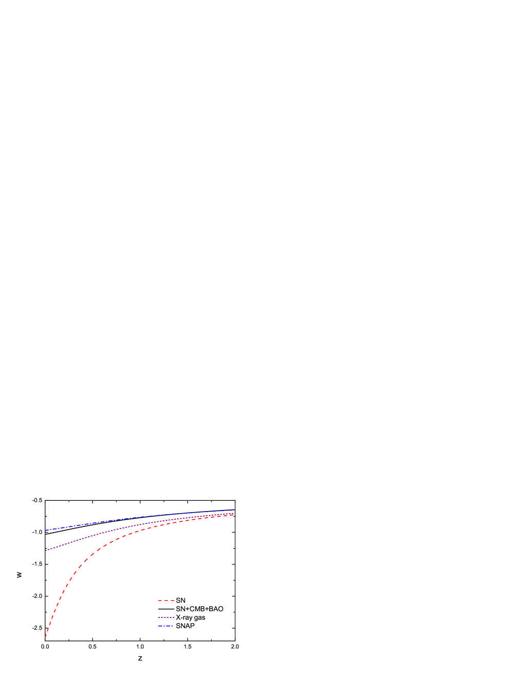
Figure 1: The evolutions of the equation of state of holographic dark energy. Here we use the best fit results of the type Ia supernovae, the joint analysis of SN+CMB+BAO, the X-ray gas mass fraction of galaxy clusters, and the Monte Carlo simulation of SNAP mission, respectively. In the concrete, $c=0.21$ and $\Omega_{\rm m}^{0}=0.47$ for SN; $c=0.81$ and $\Omega_{\rm m}^{0}=0.28$ for SN+CMB+BAO; $c=0.61$ and $\Omega_{\rm m}^{0}=0.24$ for X-ray gas; $c=0.92$ and $\Omega_{\rm m}^{0}=0.23$ for SNAP.

As has been analyzed above, the holographic dark energy scenario reveals the dynamical nature of the vacuum energy. When taking the holographic principle into account, the vacuum energy density will evolve dynamically. In particular, the analysis of the observational data indicates that the holographic vacuum energy is likely to behave as quintom dark energy. On the other hand, as has already mentioned, the scalar field dark energy models are often viewed as effective description of the underlying theory of dark energy. However, the underlying theory of dark energy can not be achieved before a complete theory of quantum gravity is established. We can, nevertheless, speculate on the underlying theory of dark energy by taking some principles of quantum gravity into account. The holographic dark energy model is no doubt a tentative in this way. We are now interested in that if we assume the holographic vacuum energy scenario as the underlying theory of dark energy, how the scalar field model can be used to effectively describe it.

It should be pointed out that the quintom type dark energy whose equation-of-state crosses the cosmological-constant boundary ($w=-1$) can not be realized by an ordinary minimally coupled scalar field [$p=X-V(\phi)$]. This transition of crossing $w=-1$ can occur for the Lagrangian density $p(\phi,X)$ in which $\partial{p}/\partial{X}$ changes sign from positive to negative, but we require nonlinear terms in $X$ to realize the $w=-1$ crossing [29, 30]. It has been shown in Ref.[30] that a simple one-field model, generalized ghost condensate, can easily realize the crossing cosmological-constant boundary. We shall use this scalar field model to effectively describe the holographic quintom vacuum energy, and perform the reconstruction of such a scalar model. For the reconstruction of dark energy models, see e.g. [30, 31, 32, 33, 34, 35, 36, 37].

First, let us consider the Lagrangian density of a general scalar field $p(\phi,X)$, where $X=-g^{\mu\nu}\partial_{\mu}\phi\partial_{\nu}\phi/2$ is the kinetic energy term. Note that $p(\phi,X)$ is a general function of $\phi$ and $X$, and we have used a sign notation $(-,+,+,+)$. Identifying the energy momentum tensor of the scalar field with that of a perfect fluid, we can easily derive the energy density, $\rho_{\rm de}=2Xp_{X}-p$, where $p_{X}=\partial p/\partial X$. Thus, in a spatially flat FRW universe, the dynamic equations for the scalar field are

$$3H^{2}=\rho_{\rm m}+2Xp_{X}-p,$$ (10)

$$2\dot{H}=-\rho_{\rm m}-2Xp_{X},$$ (11)

where $X=\dot{\phi}^{2}/2$ in the cosmological context. Introducing a dimensionless quantity

$$r\equiv H^{2}/H_{0}^{2},$$ (12)

we find from Eqs.(10) and (11) that

$$p=[(1+z)r^{\prime}-3r]H_{0}^{2},$$ (13)

$$\phi^{\prime 2}p_{X}={r^{\prime}-3\Omega_{\rm m}^{0}(1+z)^{2}\over r(1+z)},$$ (14)

where prime denotes a derivative with respect to $z$. The equation of state for dark energy is given by

$$w={p\over\dot{\phi}^{2}p_{X}-p}={(1+z)r^{\prime}-3r\over 3r-3\Omega_{\rm m}^{0}(1+z)^{3}}.$$ (15)

Next, if we establish a correspondence between the holographic vacuum energy and the scalar field dark energy, we should choose a scalar field model in which crossing the cosmological-constant boundary is possible. So, let us consider the generalized ghost condensate model proposed in Ref.[30], with the Lagrangian density

$$p=-X+h(\phi)X^{2},$$ (16)

where $h(\phi)$ is a function in terms of $\phi$. Dilatonic ghost condensate model [12] corresponds to a choice $h(\phi)=ce^{\lambda\phi}$. From Eqs. (13) and (14) we obtain

$$\phi^{\prime 2}={12r-3(1+z)r^{\prime}-3\Omega_{\rm m}^{0}(1+z)^{3}\over r(1+z)^{2}},$$ (17)

$$h(\phi)={6(2(1+z)r^{\prime}-6r+r(1+z)^{2}\phi^{\prime 2})\over r^{2}(1+z)^{4}\phi^{\prime 4}}\rho_{\rm c0}^{-1},$$ (18)

where $\rho_{\rm c0}=3H_{0}^{2}$ represents the present critical density of the universe. The generalized ghost condensate describes the holographic vacuum energy, provided that

$$r={\Omega_{\rm m}^{0}(1+z)^{3}\over 1-\Omega_{\rm de}},$$ (19)

$$r^{\prime}={\Omega_{\rm m}^{0}(1+z)^{2}\over 1-\Omega_{\rm de}}\left[3-\Omega_{\rm de}\left(1+{c\over 2}\sqrt{\Omega_{\rm de}}\right)\right],$$ (20)

where $\Omega_{\rm de}$ satisfies the deferential equation (8).

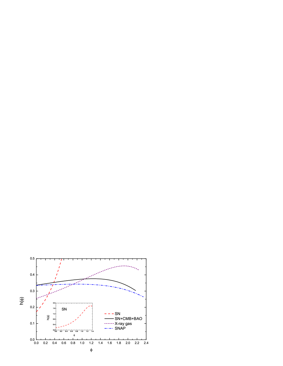
Figure 2: Reconstruction of the generalized ghost condensate model according to the holographic dark energy scenario. In this plot, we show the cases of function $h(\phi)$, in unit of $\rho_{\rm c0}^{-1}$, corresponding to the best fit results of SN, SN+CMB+BAO, X-ray gas and SNAP, respectively.

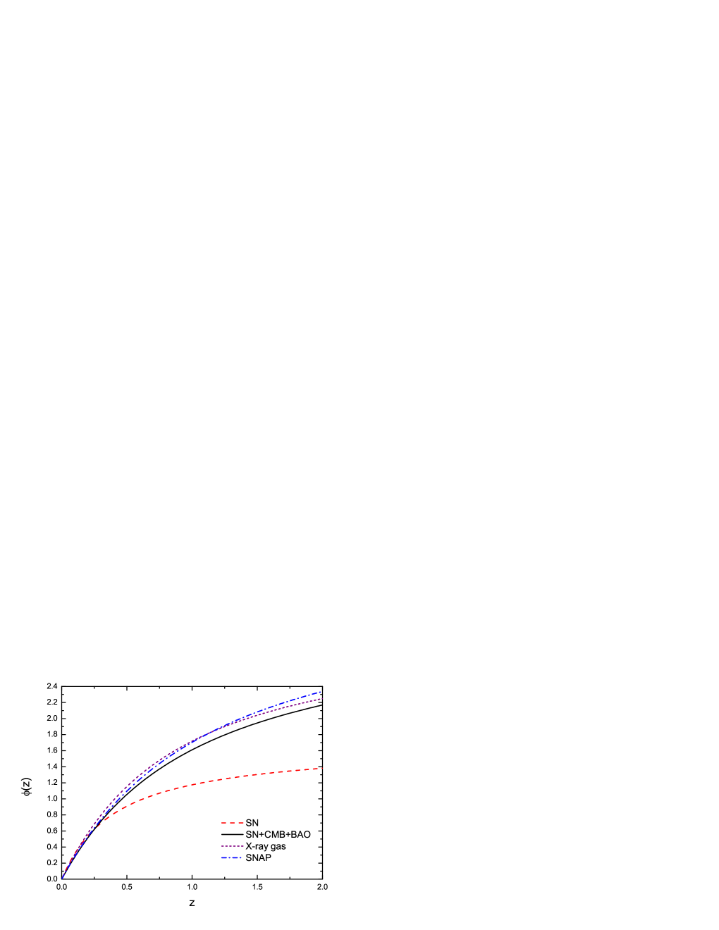
Figure 3: Reconstruction of the generalized ghost condensate model according to the holographic dark energy scenario. In this plot, we show the evolutions of the scalar field $\phi(z)$, corresponding to the best fit results of SN, SN+CMB+BAO, X-ray gas and SNAP, respectively.

The reconstruction for $h(\phi)$ is plotted in Fig.2, using the best-fit values of $c$ and $\Omega_{\rm m}^{0}$ from the observational data analyses of SN Ia, SN+CMB+BAO, X-ray gas and SNAP (simulation), respectively. The crossing of the cosmological-constant boundary corresponds to $hX=1/2$. The system can enter the phantom region ($hX<1/2$) without discontinuous behavior of $h$ and $X$. In addition, the evolution of the scalar field $\phi(z)$ is also determined by the reconstruction program, see Fig.3. It should be mentioned that the reconstruction of the generalized ghost condensate model has been carried out in Ref.[30] by using the best-fit results of the parametrization for the Hubble parameter $r(x)=\Omega_{\rm m}^{0}x^{3}+A_{0}+A_{1}x+A_{2}x^{2}$, where $x=1+z$ and $A_{0}=1-A_{1}-A_{2}-\Omega_{\rm m}^{0}$, from the SN Gold dataset [25]. Our reconstruction result is consistent with that of Ref.[30], except for the $c=0.21$ case (since the SN fit result for the holographic dark energy model is not reasonable, for details see Ref.[21]). The future high-precision observations are expected to determine the value of $c$ and the functional form of $h(\phi)$ more accurately.

In conclusion, we suggest in this paper a correspondence between the holographic dark energy scenario and a scalar field dark energy model. We adopt the viewpoint of that the scalar field models of dark energy are effective theories of an underlying theory of dark energy. The underlying theory, though has not been achieved presently, is presumed to possess some features of a quantum gravity theory, which can be explored speculatively by taking into account the holographic principle of quantum gravity theory. Consequently, the vacuum energy acquires the dynamical property when imposing the holographic principle. Moreover, the current available observational data imply that the holographic vacuum energy behaves as quintom-type dark energy, i.e. the equation-of-state of dark energy crosses the cosmological-constant boundary $w=-1$ during the evolution history. If we regard the scalar field model as an effective description of such a theory (holographic vacuum), we should be capable of using the scalar field model to mimic the evolving behavior of the dynamical vacuum energy and reconstructing this scalar field model according to the fits of the observational dataset. We find the generalized ghost condensate model is a good choice for depicting the holographic vacuum energy, since it can easily realize the quintom behavior. We thus reconstructed the function $h(\phi)$ of the generalized ghost condensate model using the best-fit results of the observational data. We hope that the future high precision observations (e.g. SNAP) may be capable of determining the fine property of the dark energy and consequently reveal some significant features of the underlying theory of dark energy.

References

-
[1]
M. Tegmark et al. [SDSS Collaboration],
Phys. Rev. D 69, 103501 (2004)
[astro-ph/0310723];
K. Abazajian et al. [SDSS Collaboration], Astron. J. 128, 502 (2004) [astro-ph/0403325];
K. Abazajian et al. [SDSS Collaboration], Astron. J. 129, 1755 (2005) [astro-ph/0410239]. -
[2]
A. G. Riess et al. [Supernova Search Team Collaboration],
Astron. J. 116, 1009 (1998)
[astro-ph/9805201];
S. Perlmutter et al. [Supernova Cosmology Project Collaboration], Astrophys. J. 517, 565 (1999) [astro-ph/9812133];
P. Astier et al., Astron. Astrophys. 447, 31 (2006) [astro-ph/0510447]. -
[3]
D. N. Spergel et al. [WMAP Collaboration],
Astrophys. J. Suppl. 148, 175 (2003)
[astro-ph/0302209];
D. N. Spergel et al., astro-ph/0603449. - [4] A. Einstein, Sitzungsber. K. Preuss. Akad. Wiss. 142 (1917) [Einglish translation in The Principle of Relativity (Dover, New York, 1952), p. 177].
-
[5]
S. Weinberg,
Rev. Mod. Phys. 61 1 (1989);
V. Sahni and A. A. Starobinsky, Int. J. Mod. Phys. D 9, 373 (2000) [astro-ph/9904398];
S. M. Carroll, Living Rev. Rel. 4 1 (2001) [astro-ph/0004075];
P. J. E. Peebles and B. Ratra, Rev. Mod. Phys. 75 559 (2003) [astro-ph/0207347];
T. Padmanabhan, Phys. Rept. 380 235 (2003) [hep-th/0212290]. - [6] P. J. Steinhardt, in Critical Problems in Physics, edited by V. L. Fitch and D. R. Marlow (Princeton University Press, Princeton, NJ, 1997).
-
[7]
P. J. E. Peebles and B. Ratra,
Astrophys. J. 325 L17 (1988);
B. Ratra and P. J. E. Peebles, Phys. Rev. D 37 3406 (1988);
C. Wetterich, Nucl. Phys. B 302 668 (1988);
J. A. Frieman, C. T. Hill, A. Stebbins and I. Waga, Phys. Rev. Lett. 75, 2077 (1995) [astro-ph/9505060];
M. S. Turner and M. J. White, Phys. Rev. D 56, 4439 (1997) [astro-ph/9701138];
R. R. Caldwell, R. Dave and P. J. Steinhardt, Phys. Rev. Lett. 80, 1582 (1998) [astro-ph/9708069];
A. R. Liddle and R. J. Scherrer, Phys. Rev. D 59, 023509 (1999) [astro-ph/9809272];
I. Zlatev, L. M. Wang and P. J. Steinhardt, Phys. Rev. Lett. 82, 896 (1999) [astro-ph/9807002];
P. J. Steinhardt, L. M. Wang and I. Zlatev, Phys. Rev. D 59, 123504 (1999) [astro-ph/9812313]. -
[8]
C. Armendariz-Picon, V. F. Mukhanov and P. J. Steinhardt,
Phys. Rev. Lett. 85, 4438 (2000)
[astro-ph/0004134];
C. Armendariz-Picon, V. F. Mukhanov and P. J. Steinhardt, Phys. Rev. D 63, 103510 (2001) [astro-ph/0006373]. -
[9]
A. Sen,
JHEP 0207, 065 (2002)
[hep-th/0203265];
T. Padmanabhan, Phys. Rev. D 66, 021301 (2002) [hep-th/0204150]. -
[10]
R. R. Caldwell,
Phys. Lett. B 545, 23 (2002)
[astro-ph/9908168];
R. R. Caldwell, M. Kamionkowski and N. N. Weinberg, Phys. Rev. Lett. 91, 071301 (2003) [astro-ph/0302506]. - [11] N. Arkani-Hamed, H. C. Cheng, M. A. Luty and S. Mukohyama, JHEP 0405, 074 (2004) [hep-th/0312099].
- [12] F. Piazza and S. Tsujikawa, JCAP 0407, 004 (2004) [hep-th/0405054].
-
[13]
B. Feng, X. L. Wang and X. M. Zhang,
Phys. Lett. B 607, 35 (2005)
[astro-ph/0404224];
B. Feng, M. Li, Y. S. Piao and X. M. Zhang, Phys. Lett. B 634, 101 (2006) [astro-ph/0407432];
Z. K. Guo, Y. S. Piao, X. M. Zhang and Y. Z. Zhang, Phys. Lett. B 608, 177 (2005) [astro-ph/0410654];
X. Zhang, Commun. Theor. Phys. 44, 762 (2005);
X. F. Zhang, H. Li, Y. S. Piao and X. M. Zhang, Mod. Phys. Lett. A 21, 231 (2006) [astro-ph/0501652];
H. Wei, R. G. Cai and D. F. Zeng, Class. Quant. Grav. 22, 3189 (2005) [hep-th/0501160];
M. Z. Li, B. Feng and X. M. Zhang, JCAP 0512, 002 (2005) [hep-ph/0503268];
A. Anisimov, E. Babichev and A. Vikman, JCAP 0506, 006 (2005) [astro-ph/0504560];
H. Wei and R. G. Cai, Phys. Lett. B 634, 9 (2006) [astro-ph/0512018];
H. Wei and R. G. Cai, Phys. Rev. D 73, 083002 (2006) [astro-ph/0603052];
Z. K. Guo, Y. S. Piao, X. Zhang and Y. Z. Zhang, astro-ph/0608165;
Y. F. Cai, H. Li, Y. S. Piao and X. M. Zhang, gr-qc/0609039. - [14] E. Witten, hep-ph/0002297.
- [15] A. G. Cohen, D. B. Kaplan and A. E. Nelson, Phys. Rev. Lett. 82, 4971 (1999) [hep-th/9803132].
-
[16]
P. Horava and D. Minic,
Phys. Rev. Lett. 85, 1610 (2000)
[hep-th/0001145];
S. D. Thomas, Phys. Rev. Lett. 89, 081301 (2002). - [17] S. D. H. Hsu, Phys. Lett. B 594, 13 (2004) [hep-th/0403052].
- [18] M. Li, Phys. Lett. B 603, 1 (2004) [hep-th/0403127].
-
[19]
G. ’t Hooft,
gr-qc/9310026;
L. Susskind, J. Math. Phys. 36, 6377 (1995) [hep-th/9409089]. -
[20]
J. D. Bekenstein, Phys. Rev. D 7 (1973) 2333;
J. D. Bekenstein, Phys. Rev. D 9 (1974) 3292; J. D. Bekenstein, Phys. Rev. D 23 (1981) 287;
J. D. Bekenstein, Phys. Rev. D 49 (1994) 1912;
S. W. Hawking, Commun. Math. Phys. 43 (1975) 199;
S. W. Hawking, Phys. Rev. D 13 (1976) 191. - [21] X. Zhang and F. Q. Wu, Phys. Rev. D 72, 043524 (2005) [astro-ph/0506310].
- [22] Z. Chang, F. Q. Wu and X. Zhang, Phys. Lett. B 633, 14 (2006) [astro-ph/0509531].
-
[23]
Q. G. Huang and Y. G. Gong,
JCAP 0408, 006 (2004)
[astro-ph/0403590];
K. Enqvist, S. Hannestad and M. S. Sloth, JCAP 0502 004 (2005) [astro-ph/0409275];
J. Shen, B. Wang, E. Abdalla and R. K. Su, Phys. Lett. B 609 200 (2005) [hep-th/0412227];
H. C. Kao, W. L. Lee and F. L. Lin, Phys. Rev. D 71 123518 (2005) [astro-ph/0501487]. -
[24]
Q. G. Huang and M. Li,
JCAP 0408, 013 (2004)
[astro-ph/0404229];
K. Enqvist and M. S. Sloth, Phys. Rev. Lett. 93, 221302 (2004) [hep-th/0406019];
K. Ke and M. Li, Phys. Lett. B 606, 173 (2005) [hep-th/0407056];
Q. G. Huang and M. Li, JCAP 0503, 001 (2005) [hep-th/0410095];
X. Zhang, Int. J. Mod. Phys. D 14, 1597 (2005) [astro-ph/0504586];
D. Pavon and W. Zimdahl, Phys. Lett. B 628, 206 (2005) [gr-qc/0505020];
B. Wang, Y. Gong and E. Abdalla, Phys. Lett. B 624, 141 (2005) [hep-th/0506069];
H. Kim, H. W. Lee and Y. S. Myung, Phys. Lett. B 632, 605 (2006) [gr-qc/0509040];
S. Nojiri and S. D. Odintsov, Gen. Rel. Grav. 38, 1285 (2006) [hep-th/0506212];
E. Elizalde, S. Nojiri, S. D. Odintsov and P. Wang, Phys. Rev. D 71, 103504 (2005) [hep-th/0502082];
B. Hu and Y. Ling, Phys. Rev. D 73, 123510 (2006) [hep-th/0601093];
H. Li, Z. K. Guo and Y. Z. Zhang, Int. J. Mod. Phys. D 15, 869 (2006) [astro-ph/0602521];
M. R. Setare and S. Shafei, JCAP 0609, 011 (2006) [gr-qc/0606103];
M. R. Setare, Phys. Lett. B 642, 1 (2006) [hep-th/0609069];
M. R. Setare, hep-th/0609104;
H. M. Sadjadi and M. Honardoost, gr-qc/0609076. - [25] U. Alam, V. Sahni and A. A. Starobinsky, JCAP 0406, 008 (2004) [astro-ph/0403687].
- [26] D. Huterer and A. Cooray, Phys. Rev. D 71, 023506 (2005) [astro-ph/0404062].
- [27] A. G. Riess et al. [Supernova Search Team Collaboration], Astrophys. J. 607, 665 (2004) [astro-ph/0402512].
- [28] D. J. Eisenstein et al. [SDSS Collaboration], Astrophys. J. 633, 560 (2005) [astro-ph/0501171].
- [29] A. Vikman, Phys. Rev. D 71, 023515 (2005) [astro-ph/0407107].
-
[30]
S. Tsujikawa, Phys. Rev. D 72, 083512 (2005)
[astro-ph/0508542];
E. J. Copeland, M. Sami and S. Tsujikawa, hep-th/0603057. - [31] T. D. Saini, S. Raychaudhury, V. Sahni and A. A. Starobinsky, Phys. Rev. Lett. 85, 1162 (2000) [astro-ph/9910231].
-
[32]
A. A. Starobinsky, JETP Lett. 68, 757 (1998) [Pis’ma Zh. Eksp.
Teor. Fiz. 68, 721 (1998)] [astro-ph/9810431];
D. Huterer and M. S. Turner, Phys. Rev. D 60, 081301 (1999) [astro-ph/9808133];
T. Nakamura and T. Chiba, Mon. Not. R. Astron. Soc. 306, 696 (1999) [astro-ph/9810447]. - [33] B. Boisseau, G. Esposito-Farese, D. Polarski and A. A. Starobinsky, Phys. Rev. Lett. 85, 2236 (2000) [gr-qc/0001066].
-
[34]
M. Szydlowski and W. Czaja,
Phys. Rev. D 69, 083518 (2004)
[gr-qc/0305033];
M. Szydlowski and W. Czaja, Phys. Rev. D 69, 083507 (2004) [astro-ph/0309191]. - [35] X. Zhang, astro-ph/0604484.
-
[36]
Z. K. Guo, N. Ohta and Y. Z. Zhang,
Phys. Rev. D 72, 023504 (2005)
[astro-ph/0505253];
H. Li, Z. K. Guo and Y. Z. Zhang, Mod. Phys. Lett. A 21, 1683 (2006) [astro-ph/0601007];
Z. K. Guo, N. Ohta and Y. Z. Zhang, astro-ph/0603109. - [37] W. Zhao and Y. Zhang, Phys. Rev. D 73, 123509 (2006) [astro-ph/0604460].