Gravitational Lens Time Delays: A Statistical Assessment of Lens Model Dependences and Implications for the Global Hubble Constant

Abstract

Time delays between lensed multiple images have been known to provide an interesting probe of the Hubble constant, but such application is often limited by degeneracies with the shape of lens potentials. We propose a new statistical approach to examine the dependence of time delays on the complexity of lens potentials, such as higher-order perturbations, non-isothermality, and substructures. Specifically, we introduce a reduced time delay of the dimensionless form, and explore its behavior analytically and numerically as a function of the image configuration that is characterized by the asymmetry and opening angle of the image pair. In particular we derive a realistic conditional probability distribution for a given image configuration from Monte-Carlo simulations. We find that the probability distribution is sensitive to the image configuration such that more symmetric and/or smaller opening angle image pairs are more easily affected by perturbations on the primary lens potential. On average time delays of double lenses are less scattered than those of quadruple lenses. Furthermore, the realistic conditional distribution allows a new statistical method to constrain the Hubble constant from observed time delays. We find that 16 published time delay quasars constrain the Hubble constant to be $H_{0}=70\pm 6\,{\rm km\,s^{-1}Mpc^{-1}}$, where the value and its error are estimated using jackknife resampling. Systematic errors coming from the heterogeneous nature of the quasar sample and the uncertainty of the input distribution of lens potentials can be larger than the statistical error. After including rough estimates of the sizes of important systematic errors, we find $H_{0}=68\pm 6({\rm stat.})\pm 8({\rm syst.})\,{\rm km\,s^{-1}Mpc^{-1}}$. The reasonable agreement of the value of the Hubble constant with other estimates indicates the usefulness of our new approach as a cosmological and astrophysical probe, particularly in the era of large-scale synoptic surveys.

1. Introduction

It has been known that time delays between multiple images of strong gravitational lens systems offer an interesting method to measure the Hubble constant $H_{0}$, the most fundamental cosmological parameter that governs the length and time scale of our universe (Refsdal, 1964). A huge advantage of this method is that it does not rely on so-called distance ladder and can measure the global Hubble constant independently of any local measurements. Motivated by this time delays have been measured in more than 10 lensed quasar systems (see, e.g., Kochanek, 2006). The situation as it presents is, however, somewhat confusing and controversial. Kochanek (2002, 2003) claimed from the analysis of several lens systems that the Hubble constant should be relatively low, $H_{0}\sim 50\,{\rm km\,s^{-1}Mpc^{-1}}$. The time delay of SDSS J1650+4251 also prefers the low Hubble constant (Vuissoz et al., 2007). On the other hand, Koopmans et al. (2003) performed systematic mass modeling of B1608+656 using all available data from radio to optical and found constrained the value of the Hubble constant to be $H_{0}=75^{+7}_{-6}\,{\rm km\,s^{-1}Mpc^{-1}}$. The analysis of the smallest separation lens B0218+357 yields $H_{0}=78\pm 3\,{\rm km\,s^{-1}Mpc^{-1}}$ (Wucknitz et al., 2004). By combining time delays in 10 lensed quasar systems Saha et al. (2006) obtained $H_{0}=72^{+8}_{-11}\,{\rm km\,s^{-1}Mpc^{-1}}$.

The large variation of derived values of the Hubble constant from time delays reflects the fact that time delays are quite sensitive to mass distributions of lens objects, which leads to strong degeneracies between lens mass profiles and the Hubble constant. The most fundamental, mathematically rigorous degeneracy is the mass-sheet degeneracy (Falco et al., 1985); inserting an uniform sheet instead of decreasing the mass normalization of lenses changes estimated values of the Hubble constant while leaving unchanged the image observables. This degeneracy implies that the derived values of the Hubble constant also degenerates with radial density profiles of of lens galaxies (Refsdal & Surdej, 1994; Witt et al., 1995; Keeton & Kochanek, 1997; Witt et al., 2000; Saha, 2000; Tada & Futamase, 2000; Wucknitz, 2002; Treu & Koopmans, 2002; Kochanek, 2002, 2003; Oguri & Kawano, 2003; Rusin et al., 2003; Schechter, 2005; Mörtsell et al., 2005; Kawano & Oguri, 2006). In addition, it may degenerate with the angular structure of lenses as well (Zhao & Qin, 2003; Saha & Williams, 2006). The sensitivity of time delays on mass profiles suggests that by assuming the Hubble constant, which can be determined by other methods (Freedman et al., 2001; Tegmark et al., 2006; Spergel et al., 2007), we can put constraints on mass distributions of lenses, in particular radial density profiles (e.g., Oguri et al., 2004; Kochanek et al., 2006b; Dobke & King, 2006).

One way to overcome the degeneracies is to adopt lens systems whose lens potentials can well be constrained by many observational constraints. An example of such constraints comes from lensed images of quasar host galaxies. The lensed host galaxies often form Einstein rings, which accurately and independently determines the structure of the lens potential as well as the shape of the lensed host galaxy (e.g., Keeton et al., 2000; Kochanek et al., 2001; Koopmans et al., 2003). The small-scale structure of lensed quasars, such as radio jets and sub-components, determine lens potentials in a similar way as Einstein rings (e.g., Cohn et al., 2001; Wucknitz et al., 2004). Furthermore, the measurement of velocity dispersions of lens galaxies serves as useful constraints on mass distributions, helping to break degeneracies between mass models (e.g., Treu & Koopmans, 2002). Lens systems for which these strong additional constraints are available, sometime referred as “golden lenses”, have been thought to be an effective probe of the Hubble constant.

Another potentially powerful, but less studied, method to measure the Hubble constant is a statistical approach. Even if each individual lens lacks strong constraints that allow detailed investigations of the mass distribution, by combining many lens systems one can put tight constraints on the Hubble constant. As mentioned above, this approach was in some sense demonstrated recently by Saha et al. (2006) who combined 10 lensed quasar systems to constrain the Hubble constant. A caveat is that lensed quasars sometimes suffer from selection effects. For instance, brighter lensed quasars with larger image separations are more likely to lie in dense environments such as groups and clusters (Oguri et al., 2005; Oguri, 2006), thus the Hubble constant from those lensed quasars may be systematically higher than the true value without any correction of the effect of dark matter along the line of sight. This indicates the importance of well-defined statistical sample of lensed quasars for which we can quantitatively estimate and correct the selection effect. While the statistical sample has been very limited so far, containing $\sim 20$ lenses even for the largest lens sample (Myers et al., 2003; Browne et al., 2003), larger lens surveys will be soon available by ongoing/future lens surveys such as done by the Sloan Digital Sky Survey (Oguri et al., 2006), the Large Synoptic Survey Telescope (LSST), and the Supernova/Acceleration Probe (SNAP). Future lens surveys will also find strong lensing of distant supernovae (e.g., Oguri et al., 2003) for which time delays can easily be measured (but see Dobler & Keeton, 2006). Therefore the statistical approach is growing its importance.

In this paper, we study how time delays depend on various properties of the lens potential and image configurations, which is essential for the determination of the Hubble constant from time delays. Using both analytic and numerical methods, we show how time delays are affected by several complexity of the lens potential, such as radial mass profiles, external perturbations, higher order multipoles, and substructures. We then derive the expected distributions of time delays by adopting realistic lens potentials. The distribution, in turn, can be used to derive statistically the value of the Hubble constant from observed time delays. This approach differs from the statistical argument by Saha et al. (2006) in the sense that they fit image positions of individual lens systems to constrain the Hubble constant and then combined results of all the lens systems: Our new approach does not even require modeling of each lens system. This has an advantage that we can include lens systems that have too few constraints to determine the lens potential. In this sense the approach is extension of study by Oguri et al. (2002) in which only spherical halos are considered to compute time delay distributions. We note that the methodology is similar to that adopted by Keeton et al. (2003, 2005) who derived distributions of flux ratios of image pairs to identify small-scale structure in lens galaxies.

In addition to the measurement of the Hubble constant, the sensitivity of time delays on mass models, which we explore in this paper, offers guidance on the usefulness of each time delay measurement as a cosmological or astrophysical probe: If time delays at some image configuration is quite sensitive to detailed structure of the lens such as higher-order multipole terms with small amplitudes or substructures, which are difficult to be constrained even for best-studied lens systems, it is almost hopeless to use these time delays to extract either radial mass profiles or the Hubble constant. Our result can be used to assess quantitatively which lens systems are more suitable for detailed studies, i.e., less sensitive to the complexity of the lens potential. There has been several insightful analytic work (e.g., Witt et al., 2000; Kochanek, 2002), but here we perform more systematic and comprehensive survey of model dependences of time delays by parameterizing image configurations of lensed quasar systems using dimensionless quantities.

This paper is organized as follows. In §2 we introduce several dimensionless quantities that are used to explore the model dependence of time delays. We study the sensitivity of time delays on the various lens potentials analytically in §3. Section 4 is devoted to construct the conditional distribution of time delays from realistic Monte-Carlo simulations. We compare it with observed time delays in §5, and constrain the Hubble constant in §6. Finally discussion of our results and conclusion are given in §7. Throughout the paper we adopt a flat universe with the matter density $\Omega_{M}=0.24$ and the cosmological constant $\Omega_{\Lambda}=0.76$ (Tegmark et al., 2006), although our results are only weakly dependent on the specific choice of the cosmological parameters. The Hubble constant is sometimes described by the dimensionless form $h\equiv H_{0}/(100\,{\rm km\,s^{-1}Mpc^{-1}})$.

2. Characterizing Time Delay Quasars

Let us consider a lens system in which a source at ${\mathbf{u}}=(u,v)$ is multiply imaged at the image positions ${\mathbf{x}}_{i}=(x_{i},y_{i})$. We also use the polar coordinates for the image positions, ${\mathbf{x}}_{i}=(x_{i},y_{i})=(r_{i}\cos\theta_{i},r_{i}\sin\theta_{i})$. We always choose the center of the lens object as the origin of the coordinates. Time delays between these multiply images are given by (e.g., Blandford & Narayan, 1986)

$$\Delta t_{ij} = \frac{1+z_{l}}{2c}\frac{D_{\rm ol}D_{\rm os}}{D_{\rm ls}}$$ (1)

$$\times\left[({\mathbf{x}}_{i}-{\mathbf{u}})^{2}-({\mathbf{x}}_{j}-{\mathbf{u}})^{2}-2\phi({\mathbf{x}}_{i})+2\phi({\mathbf{x}}_{j})\right],$$

where $z_{l}$ is the redshift of the lens, $c$ is the speed of light, and $D_{\rm ol}$, $D_{\rm os}$, and $D_{\rm ls}$ are angular diameter distances from the observer to the lens, from the observer to the source, and from the lens to the source, respectively. The lens potential $\phi({\mathbf{x}})$ is related to the surface mass density of the lens $\Sigma({\mathbf{x}})$ by the Poisson equation:

$$\nabla^{2}\phi({\mathbf{x}})=2\kappa({\mathbf{x}})=2\frac{\Sigma({\mathbf{x}})}{\Sigma_{\rm crit}},$$ (2)

with $\Sigma_{\rm crit}=c^{2}D_{\rm os}/(4\pi GD_{\rm ol}D_{\rm ls})$ being the critical surface mass density ($G$ is the gravitational constant). Note that image positions and source positions are related by the lens equation

$${\mathbf{u}}={\mathbf{x}}_{i}-\nabla\phi({\mathbf{x}}_{i}).$$ (3)

Equation (1) involves unobservable quantities such as ${\mathbf{u}}$ and $\phi({\mathbf{x}})$, indicating that time delays in general depend on details of mass models. However, Witt et al. (2000) has shown that for generalized isothermal potential

$$\phi({\mathbf{x}})=rF(\theta),$$ (4)

where $F(\theta)$ is an arbitrary function of $\theta$, time delays can be expressed in a very simple form involving only the observed image positions:

$$\Delta t_{ij}=\frac{1+z_{l}}{2c}\frac{D_{\rm ol}D_{\rm os}}{D_{\rm ls}}(r_{j}^{2}-r_{i}^{2}),$$ (5)

where $r_{i}$ denote the distance of image $i$ from the center of the lens galaxy. Motivated by this analytic result, in this paper we consider the reduced time delay that is defined by:

$$\Xi \equiv \left|\frac{\Delta t_{ij}}{r_{j}^{2}-r_{i}^{2}}\right|\frac{2c}{1+z_{l}}\frac{D_{\rm ls}}{D_{\rm ol}D_{\rm os}}$$ (6)

$$= \left|\frac{({\mathbf{x}}_{i}-{\mathbf{u}})^{2}-({\mathbf{x}}_{j}-{\mathbf{u}})^{2}-2\phi({\mathbf{x}}_{i})+2\phi({\mathbf{x}}_{j})}{r_{j}^{2}-r_{i}^{2}}\right|.$$

In this definition, the reduced time delay $\Xi$ is always unity if the lens potential can be expressed by equation (4), but can deviate from unity if the lens potential has more complicated structures. In particular, from the analysis of Kochanek (2002) we obtain $\Xi=2(1-\langle\kappa\rangle)$ at the lowest order of expansion, where $\langle\kappa\rangle$ is the average surface density in the annulus bounded by the images. This indicates that the deviation from the isothermal mass distribution has a direct impact on the reduced time delay. But as we will see later it is affected to some extent by other factors such as external perturbations or small-scale structures as well. Thus we can regard the reduced time delay as a measure of the complexity of the lens. In addition, equation (6) indicates that we can compute reduced time delays for observed lensed quasar systems with measured time delays by assuming the value of the Hubble constant. In this sense, the reduced time delay $\Xi$ is a key quantity that represents a link between measured time delays of lens systems and theoretical lens models. We point out that $\Xi$ is dimensionless because time delays are proportional to the square of the size of a lens (the Einstein radius). This allows us to directly compare values of reduced time delays for different lens systems that have different sizes.

We note that Saha (2004) adopted similar but different dimensionless quantity to explore the dependence of time delays on mass models. In the paper, the parameter essentially same as equation (6) was also considered, but it was discarded because of the correlation with time delays. However, the correlation just reflects the effect of surrounding dark matter that is larger for wider separation lenses (Oguri et al., 2005; Oguri, 2006). Put another way, such correlation is naturally expected from very different mass distributions and environments between small ($\sim 1^{\prime\prime}$) and large ($\gtrsim 3^{\prime\prime}$) separation lenses. Indeed the apparent lack of the correlation between time delays and the scaled time delays in Saha (2004) comes mostly from the large scatter among different image configurations: The effect of external mass is hindered by the large scatter his parametrization involves. Therefore in this paper we propose equation (6) as useful quantity to extract the mass dependences on time delays.

Previous analytic calculations of time delays suggest that the model dependence of time delays is a strong function of image configurations (Witt et al., 2000; Kochanek, 2002). In this paper we characterize image configurations by the following two parameters. One is the asymmetry of the images define by

$$R_{ij}\equiv\left|\frac{r_{j}-r_{i}}{r_{j}+r_{i}}\right|.$$ (7)

Again, $R_{ij}$ is dimensionless and does not depend on the size of the lens: $R_{ij}\sim 0$ means the images are roughly at the same distance from the lens galaxy, while $R_{ij}\sim 1$ indicates very asymmetric configurations that one image lies very close to the lens center and the other image is far apart from the lens. The other parameter we use is the opening angle of images:

$$\theta_{ij}\equiv\cos^{-1}\left(\frac{{\mathbf{x}}_{i}\cdot{\mathbf{x}}_{i}}{r_{i}r_{j}}\right).$$ (8)

In this definition, if the images are directly opposite each other, $\theta_{ij}\sim 180^{\circ}$. On the other hand, close image pairs such as merging images near cusp and fold catastrophe have $\theta_{ij}\sim 0^{\circ}$. Note that both $R_{ij}$ and $\theta_{ij}$ are observables in the sense that they can be derived without ambiguity for each observed lens system as long as the lens galaxy is identified: We do not have to perform mass modeling to compute these quantity from observations. In summary, our task of this paper is to explore model dependences of reduced time delay $\Xi$ as a function of image configurations parameterized by $R_{ij}$ and $\theta_{ij}$.

3. Analytic Examination

In this section, we analytically examine the behavior of the reduced time delay $\Xi$ (eq. [6]) for various lens potentials, before showing the distribution of $\Xi$ for realistic complicated mass distributions. For this purpose, it is convenient to study in terms of multipole expansion: We consider the lens potential of the following from

$$\phi({\mathbf{x}})=\sum\frac{c_{n}}{\beta}R_{\rm Ein}^{2-\beta}r^{\beta}\cos n(\theta-\theta_{n}),$$ (9)

where $c_{n}$ is the dimensionless amplitude and $\theta_{n}$ is the position angle. The coefficients are chosen such that $R_{\rm Ein}$ becomes the Einstein radius of the system if the amplitude of the monopole term is $c_{0}=1$. Note that an external shear (e.g., Kochanek, 1991; Keeton et al., 1997) can be described by this expression as $\beta=n=2$ and $c_{n}=-\gamma$. For this potential the reduced time delay is given by (Witt et al., 2000):

$$\Xi=\left|1+\sum 2(1-\beta)\frac{\phi({\mathbf{x}}_{j})-\phi({\mathbf{x}}_{i})}{r_{j}^{2}-r_{i}^{2}}\right|.$$ (10)

This can be rewritten as

$$\Xi=\left|1+\sum c_{n}\left(\frac{2R_{\rm Ein}}{r_{j}+r_{i}}\right)^{2-\beta}X(R_{ij},\theta_{ij})\cos(n\theta_{n}-\delta)\right|,$$ (11)

where $\delta$ and $X(R_{ij},\theta_{ij})$ are defined by

$$\tan\delta\equiv\frac{r_{j}^{\beta}\sin n\theta_{j}-r_{i}^{\beta}\sin n\theta_{i}}{r_{j}^{\beta}\cos n\theta_{j}-r_{i}^{\beta}\cos n\theta_{i}},$$ (12)

$$X(R_{ij},\theta_{ij}) \equiv \frac{1-\beta}{2\beta}\frac{1}{R_{ij}}\left[(1+R_{ij})^{2\beta}+(1-R_{ij})^{2\beta}\right.$$ (13)

$$\left.-2(1-R_{ij}^{2})^{\beta}\cos n\theta_{ij}\right]^{1/2}.$$

Here we assumed $r_{j}>r_{i}$ without loss of generality. Note that $R_{ij}$ and $\theta_{ij}$ were defined in equations (7) and (8), respectively.

The above expression of $\Xi$ (eq. [11]) has several important implications. First, $\theta_{n}$ comes only in the last cosine term, thus assuming $n\neq 0$ and $c_{n}$ is small $\Xi>1$ and $\Xi<1$ occurs equally if $\theta_{n}$ is uncorrelated with the image configuration (as we will see later, however, this is not necessarily the case). This indicates that we can reduce the effect of multipole terms by averaging many lens systems, suggesting the usefulness of our statistical approach. Second, since $2R_{\rm E}/(r_{j}+r_{i})\sim 1$ in most cases, the dependence of the potential ($\beta$) and image configurations ($R_{ij}$ and $\theta_{ij}$) on the deviation from $\Xi=1$ is encapsulated in $X(R_{ij},\theta_{ij})$, aside from the overall amplitude $c_{n}$. In what follows, we use $X(R_{ij},\theta_{ij})$ to study the behavior of $\Xi$.

First, we consider quite symmetric cases ($R_{ij}\rightarrow 0$) for which images are nearly the same distance from the lens center. Depending on the opening angles, limiting behaviors are given by

$$X(R_{ij}\rightarrow 0,\theta_{ij})\approx\left\{\begin{array}[]{ll}{\displaystyle 1-\beta}&(\cos n\theta_{ij}=1)\\ {\displaystyle\frac{1-\beta}{\sqrt{2}\beta R_{ij}}}&(\cos n\theta_{ij}=0)\\ {\displaystyle\frac{1-\beta}{\beta R_{ij}}}&(\cos n\theta_{ij}=-1).\end{array}\right.$$ (14)

Therefore, $X(R_{ij},\theta_{ij})$ diverges unless $\cos n\theta_{ij}=1$. More rigorously, we should take the limit of $R_{ij}\rightarrow 0$ and $\theta_{ij}\rightarrow 0$:

$$X(R_{ij}\rightarrow 0,\theta_{ij}\rightarrow 0)\approx(1-\beta)\left[1+\left(\frac{n\theta_{ij}}{2\beta R_{ij}}\right)^{2}\right]^{1/2},$$ (15)

indicating that the divergence at the symmetric limit can be avoided if $\theta_{ij}\ll R_{ij}$, or more appropriately $1-\cos n\theta_{ij}\ll R_{ij}^{2}$. Since close image pairs are always near the circumference of the critical curve that has a nearly circular shape centered on the lens galaxy, such pairs in general have $R_{ij}\ll\theta_{ij}$, indicating the divergence cannot be avoided for two close images. On the other hand, the divergence may not occur for opposite images ($\theta_{ij}\sim 180^{\circ}$), but only if $n$ is even number.

Inversely, if images are very asymmetric ($R_{ij}\rightarrow 1$), $X(R_{ij},\theta_{ij})$ reduces to the following simple form

$$X(R_{ij}\rightarrow 1,\theta_{ij})\approx\frac{2^{\beta-1}(1-\beta)}{\beta}.$$ (16)

This does not depends on $\theta_{ij}$, thus the opening angle is no longer important in this situation. However it shows stronger dependence on the radial slope $\beta$.

Figure 1.— The behaviors of $X(R_{ij},\theta_{ij})$ (eq. [13]) as a function of the asymmetry parameter $R_{ij}$. From thick to thin lines, the radial slope $\beta$ is changed from $0.5$ to $4.0$. From top to bottom panels, the opening angle $\theta_{ij}$ is fixed to $\cos n\theta_{ij}=-1$, $0$, and $1$, respectively.

Figure 2.— Same as Figure 1, but $X(R_{ij},\theta_{ij})$ is plotted as a function of the opening angle $\theta_{ij}$ while fixing $R_{ij}=0.1$ (top panel), $0.5$ (middle panel), and $0.9$ (bottom panel).

Finally we plot $X(R_{ij},\theta_{ij})$ for various parameter values in Figures 1 and 2. In Figure 1, $X(R_{ij},\theta_{ij})$ is plotted as a function of the asymmetry $R_{ij}$. It grows quite rapidly as $R_{ij}$ approaches to zero for $\cos n\theta_{ij}\neq 1$. It also shows stronger sensitivity on the slope $\beta$ at larger $R_{ij}$. As is clear in Figure 2, the opening angle $\theta_{ij}$ becomes more important for more symmetric lenses. All these behaviors are consistent with analytical arguments presented above.

4. Time Delays in Realistic Lens Models

In this section, we consider more realistic situations to in order to study expected spread of the reduced time delay $\Xi$ as a function of image configurations. Specifically we adopt theoretically and observationally determined distributions of lens potentials such as ellipticities, external shear, substructures, and multipole components to make predictions on realistic probability distributions of $\Xi$. The methodology is similar to that in Keeton et al. (2003, 2005) who studied cusp and fold relations to identify lenses with small-scale structure.

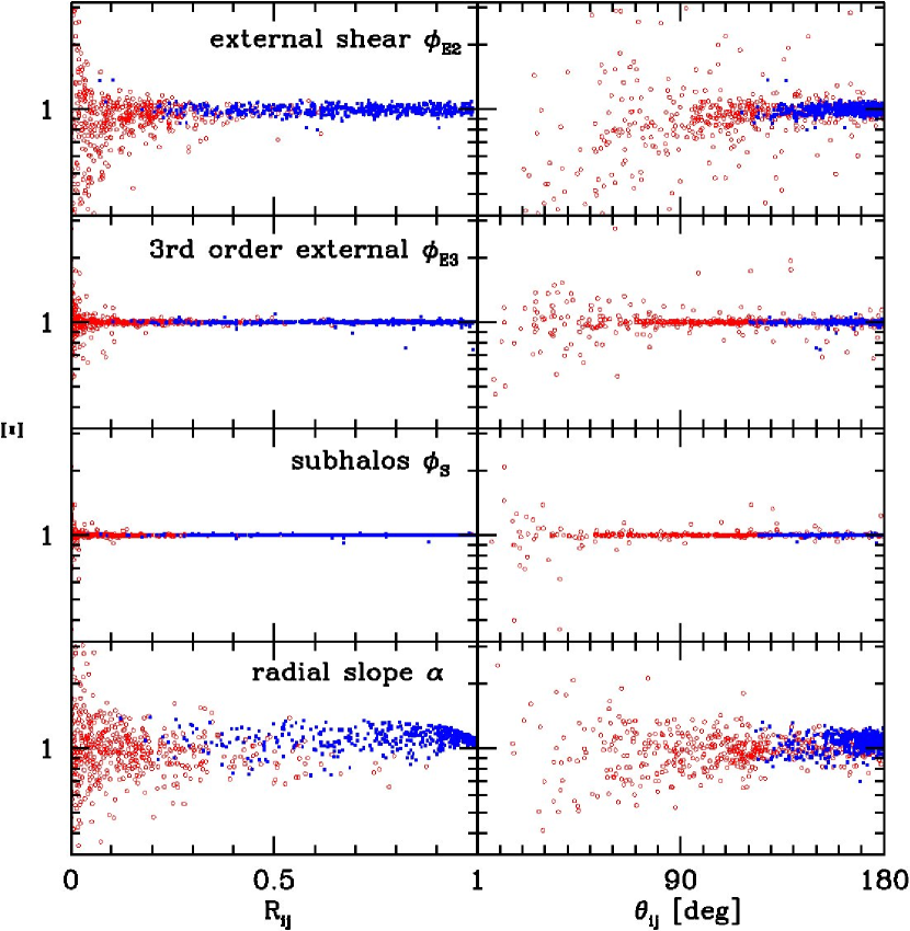
Figure 3.— Dependences of the reduced time delay $\Xi$ on several lens potentials as a function of asymmetry $R_{ij}$ (left panels) or opening angle $\theta_{ij}$ (right panels). In each panel, reduced time delays of 500 double lenses (filled squares) and 500 quadruple lenses (open circles) obtained by the Monte-Carlo simulations are plotted. Magnification bias is not considered at this stage. From top to bottom panels, we consider the external shear $\phi_{\rm E2}$ (eq. [21]), third order external perturbation $\phi_{\rm E3}$ (eq. [22]), subhalos $\phi_{\rm S}$ (eq. [24]), and non-isothermality $\alpha\neq 1$ in the primary lens potential $\phi_{\rm G}$ (eq. [19]). Besides the bottom panels, we adopt an isothermal elliptical lens as primary lens galaxies (eq. [19], $\alpha=1$) and ignore the other perturbations (e.g., in the second row we only consider $\phi_{\rm E3}$ and ignore the external shear and subhalos), thus the effect of each potential can be measured by the deviation from $\Xi=1$. In all simulations higher order multipoles (eq. [20]) are included.

4.1. Input Models

As primary lens galaxies we only consider elliptical galaxies because most ($>80$%) of quasar lenses are caused by massive elliptical galaxies (e.g., Turner et al., 1984; Kochanek, 2006; Möller et al., 2007). We model the lens galaxy as a power-law elliptical mass distribution. The surface mass distribution is given by

$$\kappa_{\rm G}({\mathbf{x}})=\frac{\alpha}{2}\left[\frac{R_{\rm Ein}}{r\sqrt{1-\epsilon\cos 2(\theta-\theta_{e})}}\right]^{2-\alpha},$$ (17)

where $R_{\rm Ein}$ is the Einstein ring radius and $\theta_{e}$ is the position angle of ellipse. The case $\alpha=1$ corresponds to the standard singular isothermal mass distribution. The ellipticity $e$, which is defined by $e=1-q$ with $q$ being the axis ratio of the ellipse, is related to $\epsilon$ by

$$\epsilon=\frac{1-(1-e)^{2}}{1+(1-e)^{2}}.$$ (18)

The corresponding lens potential can be described by

$$\phi_{\rm G}({\mathbf{x}})=\frac{1}{\alpha}R_{\rm Ein}^{2-\alpha}r^{\alpha}G(\theta),$$ (19)

with $G(\theta)$ being the complex function of $\theta$, but notice that $G(\theta)=1$ if $e=0$.

Many previous work has shown that lens galaxies indeed have nearly isothermal mass distribution. Rusin & Kochanek (2005) obtained $\alpha=0.94\pm 0.17$ by combining the Einstein radii of many lensed quasars with the fundamental plane relation of elliptical galaxies. The slope of the galaxy density profile $\alpha=1.09\pm 0.01$ constrained from the faint third image of PMN J1632$-$0033 is consistent with the nearly isothermal density profile (Winn et al., 2004). Detailed mass modeling of B1933+503 also indicates nearly isothermal profile of the lens galaxy (Cohn et al., 2001). By using measured velocity dispersions of lens galaxies of several lensed quasars, Treu & Koopmans (2004, see also ) derived $\alpha=1.25\pm 0.2$. Koopmans et al. (2006) put tighter constrains $\alpha=0.99^{+0.03}_{-0.02}$, but the results are derived from a sample of much lower redshift lens systems than typical time delay quasars. From these results, in this paper we adopt the Gaussian distribution $\alpha=1\pm 0.15$ as a conservative input distribution of the slope. For the ellipticity, we use the Gaussian distribution with median $e=0.3$ and dispersion $0.16$ that is consistent with observed distributions of isodensity contour shapes of elliptical galaxies (Bender et al., 1989; Saglia et al., 1993; Jorgensen et al., 1995; Rest et al., 2001; Sheth et al., 2003).

To allow more complex mass distribution of the galaxy, we add higher order multipole terms to the potential:

$$\phi_{\rm M}({\mathbf{x}})=\frac{1}{\alpha}R_{\rm Ein}^{2-\alpha}r^{\alpha}\sum_{m}(1-m^{2})A_{m}\cos m(\theta-\theta_{m}).$$ (20)

The factor $1-m^{2}$ is inserted such that $A_{m}$ denotes the standard parametrization for the deviation of the mass density from an ellipsoid. We include only $m=3$ and $4$ terms, because $m\geq 5$ perturbations have generally not been reported. For both $A_{3}$ and $A_{4}$, the amplitudes are distributed by the Gaussian with mean zero and dispersion $0.01$ that is roughly consistent with reported distributions (Bender et al., 1989; Saglia et al., 1993; Rest et al., 2001). It is also compatible with the level of the deviation inferred from individual modeling of lensed quasar systems (Trotter et al., 2000; Kawano et al., 2004; Kochanek & Dalal, 2004; Congdon & Keeton, 2005; Yoo et al., 2006). We assume that position angles of these multipole perturbations and that of an ellipsoid are uncorrelated with each other. In addition, we neglect the correlation of $e$ and $A_{4}$ (Keeton et al., 2003) for simplicity. Note that these multipole perturbations do not affect $\Xi$ if the lens galaxy is isothermal, $\alpha=1$, but can change quantitative results when combined with non-isothermal profiles and/or other small-scale structures. Since the effect of $A_{4}$ itself is small, we expect the effect of the correlation between $e$ and $A_{4}$, which we have neglected here, is also small.

We also include external perturbations that are known to be important for individual mass modeling (e.g., Keeton et al., 1997). The potential of lowest order external shear is given by

$$\phi_{\rm E2}({\mathbf{x}})=-\frac{\gamma}{2}r^{2}\cos 2(\theta-\theta_{\gamma}).$$ (21)

We adopt a log-normal distribution with median $\gamma=0.05$ and dispersion 0.2 dex for the distribution of shear amplitude. It is consistent with expected shear distribution from $N$-body simulations (Holder & Schechter, 2003; Dalal & Watson, 2004). In addition to external shear, we consider third order external perturbation (Kochanek, 1991; Bernstein & Fischer, 1999)

$$\phi_{\rm E3}({\mathbf{x}})=\frac{\sigma}{4}R_{\rm Ein}^{-1}r^{3}\left[\cos(\theta-\theta_{\sigma})-\cos 3(\theta-\theta_{\sigma})\right].$$ (22)

Here we assumed the external perturber is a singular isothermal object to relate the amplitudes and position angles of $n=1$ and $n=3$ terms. In general we have $\sigma\approx\gamma^{2}$ (Bernstein & Fischer, 1999), thus for the amplitude we adopt a log-normal distribution with median $\sigma=\gamma^{2}$ and dispersion 0.2 dex. The adopted amplitude is roughly consistent with values obtained from mass modeling of individual lens systems (e.g., Kawano et al., 2004). We allow small mis-alignment of the position angle $\theta_{\sigma}$, which could happen when the external perturber is not spherical, by adopting the Gaussian distribution around $\theta_{\gamma}$ with dispersion $10^{\circ}$.

Figure 4.— Contours of constant conditional probability $p(\Xi|R_{ij})$ (left panels) and $p(\Xi|\theta_{ij})$ (right panels) computed from Monte-Carlo simulations of realistic lens potentials. The contours are drawn at the 68% (solid lines), 95% (dashed lines), and 99.7% (dotted lines) confidence levels. Upper panels show the conditional probability for double lenses, whereas lower panels are for quadruple lenses. For double lenses we show $p(\Xi|\theta_{ij})$ only at $\theta_{ij}\gtrsim 110^{\circ}$ because we have too few image pairs with $\theta_{ij}\lesssim 110^{\circ}$ to construct the probability distribution.

Finally we consider substructures in the lens galaxy. A significant fraction of substructures (subhalos) in galaxies have been predicted as a natural consequence of cold dark matter cosmology (Moore et al., 1999; Klypin et al., 1999). Anomalous flux ratios observed in many gravitational lens systems indicate that substructures are indeed present (Metcalf & Madau, 2001; Chiba, 2002; Dalal & Kochanek, 2002; Bradač et al., 2002; Keeton et al., 2005; Kochanek & Dalal, 2004; Metcalf et al., 2004; Chiba et al., 2005). Note that small perturbations may also come from small halos along the line-of-sight (Keeton, 2003; Chen et al., 2003; Oguri, 2005; Metcalf, 2005). Although time delays are thought to be less sensitive to small-scale structure than flux ratios that are determined by the second derivative of the time delay surface, they might be affected to some extent particularly when two images are close to each other. We model each subhalo by pseudo-Jaffe (truncated singular isothermal) profile. The lens potential of this profile is

$$\phi_{{\rm PJ},k}({\mathbf{x}}) = b_{k}\left[r-\sqrt{r^{2}+a^{2}_{k}}\right.$$ (23)

$$\left.-\frac{a_{k}}{2}\ln\left|\frac{\sqrt{r^{2}+a^{2}_{k}}-a_{k}}{\sqrt{r^{2}+a^{2}_{k}}+a_{k}}\right|+a_{k}\ln r\right],$$

where $a_{k}$ is a truncation radius and $b_{k}$ is a mass normalization that coincides the Einstein radius for sufficiently large $a_{k}$. We adopt $a_{k}=\sqrt{b_{k}R_{\rm E}}$ assuming the truncation radius of the tidal radius of the subhalo (see, e.g., Metcalf & Madau, 2001). For the velocity distribution we assume $N(>v)=(10v/V)^{-2.7}$ inside three times the Einstein radius of the lens galaxy, where $v$ and $V$ are velocity dispersions of the subhalo and halo, respectively. The velocities can be converted to $b_{k}$ through $b_{k}/R_{\rm E}\propto(v/V)^{2}$. We distribute subhalos randomly with an uniform spatial density in the projected two-dimensional plane in order to take account of the suggested anti-bias of the subhalo spatial distribution (De Lucia et al., 2004; Mao et al., 2004; Oguri & Lee, 2004). The resulting mass fraction of subhalos at around the Einstein radius is $\sim 0.5$%, being consistent with the expectation from $N$-body simulations and analytic calculation (e.g., Mao et al., 2004; Oguri, 2005). The effect of subhalos is described by the sum of the lens potential of each subhalo:

$$\phi_{\rm S}({\mathbf{x}})=\sum_{k}\phi_{{\rm PJ},k}({\mathbf{x}}-{\mathbf{x}}_{{\rm sub},k})-\frac{1}{2}r^{2}\bar{\kappa}_{\rm sub}.$$ (24)

Here we subtracted the convergence averaged over all subhalos, $\kappa_{\rm sub}$, to conserve the total mass and radial profile of the lens galaxy. We include only 100 most massive subhalos mainly for computational reason, but small subhalos are expected to have only very small effect on time delays.

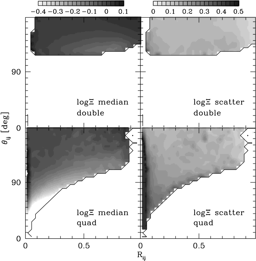
Figure 5.— Contour plot of median (left panels) and scatter (right panels) of the conditional probability $p(\Xi|R_{ij},\theta_{ij})$ in the $R_{ij}$-$\theta_{ij}$ plane. Here the scatter is defined by the 68% confidence interval width in units of $\log\Xi$. The probability distribution for double (upper panels) and quadruple (lower panels) lenses are shown separately. Thick solid lines indicate the limit beyond which the number of image pairs in Monte-Carlo simulations is too small to construct the conditional probability.

4.2. Simulation Method

Using the model described above, we perform a large Monte-Carlo simulation containing $>10^{6}$ lensed image pairs. The simulation is done by first generating a lens potential according to the distributions summarized in §4.1. All lengths are scaled by the Einstein ring radius $R_{\rm E}$: Since our results do not depend on adopted length scales, we fix $R_{\rm E}$ to unity in the simulations. We generate 10000 different lens potentials in total. For each lens potential, we place random sources with an uniform density of $\sim 100R_{\rm E}^{-2}$ in the source plane. We use a public software lensmodel (Keeton, 2001) to solve the lens equation and compute time delays between multiple images. The uniform sampling in the source plane indicates that each lens potential is automatically weighted by the lensing cross section (see Keeton et al., 2003). To account for magnification bias as well, for each source we compute the total magnification factor $\mu_{\rm tot}$, and when constructing probability distributions of reduced time delays (see below) we include a weight of $\mu_{\rm tot}^{q-1}$, where $q$ is a power-law slope of the luminosity function of source quasars. We adopt $q=2.1$ that is relevant for lenses identified by the CLASS (Myers et al., 2003).

From the ensemble of image pairs, we compute conditional probability distribution functions of the reduced time delay $\Xi$ for given values of the asymmetry $R_{ij}$ and/or opening angle $\theta_{ij}$, i.e., $p(\Xi|R_{ij})$, $p(\Xi|\theta_{ij})$, and $p(\Xi|R_{ij},\theta_{ij})$. The probability distributions are computed separately for double and quadruple lenses to see how different distributions they exhibit. In what follow we ignore central faint images that are unobserved in most cases.

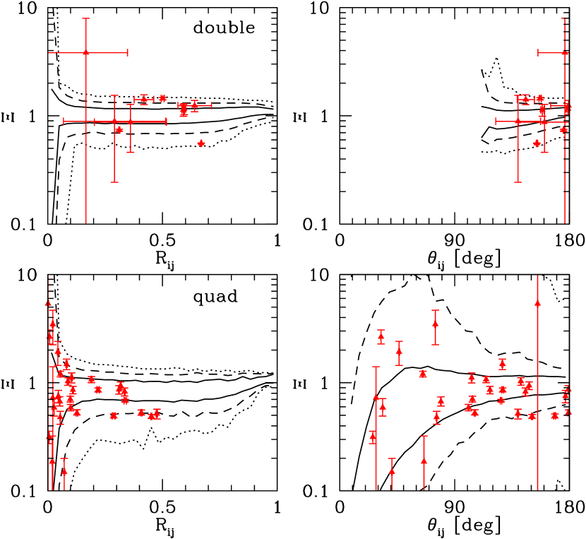
Figure 6.— Same as Figure 4, but observed values of $\Xi$ with error-bars (see Table 4.4) are plotted on the contours by filled triangles with error-bars. The Hubble constant of $h=0.73$ is assumed when computing $\Xi$ from observed time delays.

4.3. Contribution of Each Potential

Before presenting results that include all potentials, it is useful to see how each potential affects the distribution of $\Xi$. To see this we adopt isothermal elliptical lens potential plus multipole terms ($\phi_{\rm G}+\phi_{\rm M}$, $\alpha=1$), and add each lens potential: Since the isothermal galaxy always yields $\Xi=1$ (see §2) the effect of each potential term can be estimated by the deviation from $\Xi=1$. We also study the effect of non-isothermality ($\alpha\neq 1$). The results are summarized in Figure 3. First, the effect of external shear appears as a scatter around $\Xi=1$, which is consistent with discussion above (§3) as well as that of Witt et al. (2000). Both the diverging scatter at $R_{ij}\rightarrow 0$ and the modest increase of the scatter at smaller $\theta_{ij}$ are expected from our analytic examination. The scatter introduced by the third order external perturbation and subhalos is smaller than that of external shear, but it is still noticeable particularly for symmetric configurations. This means that even if we can estimate external shear and its orientation accurately for individual lens system by detailed mass modeling, these third order perturbations or subhalos can shift time delays, although these small perturbations mainly affect image pairs with small opening angles and only increase the scatter rather than shift the mean. We comment that the use of image pairs with small opening angles is also limited by the larger uncertainties of their time delay measurements. As expected, non-isothermality has a large impact on $\Xi$, but the size of its scatter is less dependent on image configurations compared with other potentials.

It is worth noting that there are systematic deviations from $\Xi=1$ for a few specific image configurations. For instance, at small $\theta_{ij}$ external shear preferentially produces image pairs with time delays smaller than the isothermal case. In addition, very asymmetric image pairs ($R_{ij}\sim 1$) tend to have larger time delays when we consider non-isothermal lens galaxies. Such systematic shifts were not predicted in our analytic arguments in §3, thus invite careful consideration. We find that the selection effect can explain these systematic shifts. For very asymmetric pairs, such configurations are possible only when the lens galaxy has a profile steeper than isothermal for which inner critical curve is degenerated at the center. If the density profile is shallower than isothermal, any images (expect central faint images that we ignore in this paper) are outside the inner critical curve. This means that very asymmetric configuration, in which one image lies very close to the center of the lens potential, never occurs for the profile shallower than isothermal. Since shallower profiles correspond to smaller $\Xi$, this increases the mean $\Xi$ at $R_{ij}\sim 1$. The effect of external shear is more complicated, but can be explained as follows. Consider a close pair of two images. If we add external shear whose position angle direction is perpendicular to the segment that connects the two images, it separates two images. On the other hand, external shear that is parallel to the segment makes the two images closer. Therefore, combined with the steep dependence of the frequency of close image pairs on the opening angle, this results in the situation that at fixed small opening angle the direction of external shear is more likely to be parallel to the segment than perpendicular. The discussion in §3 indicates that the parallel shear yields smaller time delays $\Xi<1$ for fixed image positions, thus we can conclude that close image pairs have statistically smaller time delays than those expected without external shear.

4.4. Conditional Probability Distributions

We are now ready to compute conditional probability distributions of the reduced time delay $\Xi$ with all lens potentials presented in §4.1. Figure 4 shows contours of constant conditional probability projected to one-dimensional surface, $p(\Xi|R_{ij})$ and $p(\Xi|\theta_{ij})$. The behaviors of contours can well be understood from discussions in §3 and §4.3. In particular, systematically small $\Xi$ at small opening angles and large $\Xi$ for very asymmetric image pairs, which we discussed in §4.3, are clearly seen. It appears quadruple lenses have larger scatter on average: This is because strong perturbations (external shear, third order perturbation and subhalos), which cause the scatter around $\Xi=1$, also enhance the lensing cross section for quadruple images.

To study the conditional probability distribution as a function of both $R_{ij}$ and $\theta_{ij}$, $p(\Xi|R_{ij},\theta_{ij})$, in Figure 5 we plot contours of median and 68% confidence interval of the probability distribution in the $R_{ij}$-$\theta_{ij}$ plane. The features we have discussed, such as the divergence of scatter at $R_{ij}\rightarrow 0$, smaller median time delays for small opening angle pairs, larger median time delays for asymmetric pairs, can be seen in this Figure as well. In addition, the scatter presented here is useful to check which lens systems are less dependent on lens potentials: Our result indicates that asymmetric image pairs that are collinear with their lens galaxies ($\theta_{ij}\sim 180^{\circ}$) have the least scatter and therefore are more suitable for the determination of the Hubble constant. It is interesting to note that in the statistical sense double lenses are more valuable than quadruple lenses because it shows a smaller sensitivity to various lens potentials. In addition, double lenses have advantages of easier measurements of time delays in observations and smaller fractional errors (because double lenses have longer time delays than quads). This is in contrast to individual mass modeling in which quadruple lenses are more useful because of much more observational constraints on mass models.

Table 1Summary of Observed Quasar Time Delays

Lens Name	$N_{\rm img}$	$z_{s}$	$z_{l}$	Images	$R_{ij}$	$\theta_{ij}$ [deg]	$\Delta t$ [days]	$\Xi(h=0.73)$	References
B0218+357	2	0.944	0.685	AB	$0.167\pm 0.181$	$176.5\pm 21.3$	$10.5\pm 0.2$	$3.835\pm 4.155$	1, 2, 3, 4, 5
HE0435$-$1223	4	1.689	0.455	AD	$0.099\pm 0.002$	$103.9\pm 0.2$	$14.4^{+0.9}_{-0.8}$	$0.704^{+0.045}_{-0.041}$	6, 7, 8
				AB	$0.053\pm 0.001$	$79.3\pm 0.2$	$8.0^{+0.8}_{-0.7}$	$0.671^{+0.069}_{-0.060}$
				AC	$0.002\pm 0.002$	$155.1\pm 0.2$	$2.1^{+0.7}_{-0.8}$	$5.360^{+6.070}_{-6.150}$
				BD	$0.046\pm 0.002$	$176.8\pm 0.3$	$6.4\pm 0.8$	$0.750\pm 0.100$
				CD	$0.100\pm 0.002$	$100.9\pm 0.3$	$12.3\pm 0.8$	$0.590\pm 0.040$
				BC	$0.054\pm 0.001$	$75.9\pm 0.3$	$5.9\pm 0.8$	$0.479\pm 0.066$
RXJ0911+0551	4	2.800	0.769	A1B	$0.452\pm 0.003$	$150.8\pm 0.4$	$143.0\pm 6.0$	$0.488\pm 0.021$	9, 10, 11, 12
				A2B	$0.408\pm 0.003$	$179.3\pm 0.5$	$149.0\pm 8.0$	$0.530\pm 0.029$
				A3B	$0.476\pm 0.003$	$139.6\pm 0.5$	$154.0\pm 16.0$	$0.516\pm 0.054$
SBS0909+532	2	1.377	0.830	AB	$0.291\pm 0.223$	$139.7\pm 17.6$	$45.0^{+5.5}_{-0.5}$	$0.891^{+0.657}_{-0.648}$	4, 13, 14, 15
FBQ0951+2635	2	1.246	0.260	AB	$0.591\pm 0.007$	$158.8\pm 1.2$	$16.0\pm 2.0$	$1.134\pm 0.142$	12, 16, 17, 18
Q0957+561	2	1.413	0.36	AB	$0.669\pm 0.002$	$154.5\pm 0.5$	$417.0\pm 1.5$	$0.558\pm 0.002$	19, 20, 21, 22
SDSS J1004+4112	5	1.734	0.68	AB	$0.006\pm 0.001$	$25.9\pm 0.1$	$38.4\pm 1.0$	$0.315\pm 0.041$	23, 24, 25, 26
HE1104$-$1805	2	2.319	0.729	AB	$0.312\pm 0.002$	$175.5\pm 0.3$	$152.2^{+2.8}_{-3.0}$	$0.738^{+0.015}_{-0.016}$	4, 27, 28, 29, 30
PG1115+080	4	1.735	0.310	A1B	$0.105\pm 0.003$	$103.4\pm 0.4$	$11.7\pm 1.2$	$1.115\pm 0.120$	31, 32, 33, 34, 35, 36
				A2B	$0.082\pm 0.004$	$127.5\pm 0.4$	$11.7\pm 1.2$	$1.487\pm 0.166$
				BC	$0.191\pm 0.003$	$114.7\pm 0.3$	$25.0\pm 1.6$	$1.069\pm 0.070$
				A1C	$0.088\pm 0.003$	$141.9\pm 0.3$	$13.3\pm 1.0$	$1.032\pm 0.083$
				A2C	$0.110\pm 0.003$	$117.8\pm 0.3$	$13.3\pm 1.0$	$0.857\pm 0.067$
				A1A2	$0.022\pm 0.003$	$24.1\pm 0.3$	$0.149\pm 0.006$	$0.057\pm 0.007$
RXJ1131$-$1231	4	0.658	0.295	AB	$0.008\pm 0.001$	$32.3\pm 0.1$	$12.0^{+1.5}_{-1.3}$	$2.660^{+0.411}_{-0.376}$	37, 38
				AC	$0.028\pm 0.000$	$33.7\pm 0.0$	$9.6^{+2.0}_{-1.6}$	$0.589^{+0.123}_{-0.098}$
				BC	$0.020\pm 0.001$	$66.0\pm 0.1$	$2.2\pm 1.6$	$0.187\pm 0.136$
				AD	$0.311\pm 0.002$	$179.2\pm 0.1$	$87.0\pm 8.0$	$0.863\pm 0.079$
				BD	$0.318\pm 0.002$	$148.5\pm 0.2$	$99.0\pm 8.0$	$0.940\pm 0.076$
				CD	$0.335\pm 0.002$	$145.5\pm 0.1$	$96.6\pm 8.0$	$0.825\pm 0.068$
B1422+231	4	3.620	0.337	AB	$0.023\pm 0.002$	$28.4\pm 0.2$	$1.5\pm 1.4$	$0.726\pm 0.680$	34, 39, 40
				AC	$0.022\pm 0.003$	$74.9\pm 0.3$	$7.6\pm 2.5$	$3.461\pm 1.216$
				BC	$0.045\pm 0.003$	$46.5\pm 0.3$	$8.2\pm 2.0$	$1.924\pm 0.482$
SBS1520+530	2	1.855	0.717	AB	$0.501\pm 0.007$	$157.1\pm 0.8$	$130.0\pm 3.0$	$1.444\pm 0.037$	41, 42, 43
B1600+434	2	1.589	0.414	AB	$0.640\pm 0.073$	$179.4\pm 14.2$	$51.0\pm 2.0$	$1.242\pm 0.150$	44, 45, 46, 47
B1608+656	4	1.394	0.630	AB	$0.127\pm 0.004$	$105.9\pm 0.4$	$31.5^{+2.0}_{-1.0}$	$0.525^{+0.037}_{-0.023}$	48, 49, 50, 51, 52
				BC	$0.056\pm 0.002$	$65.1\pm 0.3$	$36.0\pm 1.5$	$1.202\pm 0.072$
				BD	$0.338\pm 0.005$	$126.4\pm 0.6$	$77.0^{+2.0}_{-1.0}$	$0.681^{+0.020}_{-0.013}$
				AC	$0.072\pm 0.002$	$40.8\pm 0.2$	$4.5\pm 1.5$	$0.150\pm 0.050$
				AD	$0.220\pm 0.006$	$127.8\pm 0.7$	$45.5\pm 1.5$	$0.858\pm 0.036$
				CD	$0.287\pm 0.006$	$168.5\pm 0.7$	$41.0\pm 1.5$	$0.494\pm 0.021$
SDSS J1650+4251	2	1.547	0.577	AB	$0.420\pm 0.043$	$145.8\pm 6.8$	$49.5\pm 1.9$	$1.415\pm 0.149$	53, 54
PKS1830$-$211	2	2.507	0.89	AB	$0.360\pm 0.157$	$160.5\pm 20.3$	$26.0^{+4.0}_{-5.0}$	$0.874^{+0.401}_{-0.414}$	4, 55, 56, 57, 58
HE2149$-$2745	2	2.033	0.603	AB	$0.594\pm 0.007$	$178.9\pm 1.5$	$103.0\pm 12.0$	$1.161\pm 0.136$	12, 59, 60

Note. — All measured time delays are listed, except time delays between images A1—A3 of RXJ0911+0551 and images A—D of Q2237+030 (Vakulik et al., 2006) for which error-bars are large and therefore the detections are marginal. For Q2237+030, a possible X-ray detection of the time delay between image A and B was also reported by Dai et al. (2003). Errors indicate 1$\sigma$.

References. — (1) Patnaik et al. 1993; (2) Browne et al. 1993; (3) Biggs et al. 1999; (4) Lehár et al. 2000; (5) Cohen et al. 2003; (6) Wisotzki et al. 2002; (7) Morgan et al. 2005; (8) Kochanek et al. 2006b; (9) Bade et al. 1997; (10) Kneib et al. 2000; (11) Hjorth et al. 2002; (12) CASTLES (http://cfa-www.harvard.edu/castles/); (13) Oscoz et al. 1997; (14) Lubin et al. 2000; (15) Ullán et al. 2006; (16) Schechter et al. 1998; (17) Jakobsson et al. 2005; (18) Eigenbrod et al. 2007; (19) Walsh et al. 1979; (20) Young et al. 1981; (21) Kundic et al. 1997; (22) Barkana et al. 1999; (23) Inada et al. 2003; (24) Oguri et al. 2004; (25) Inada et al. 2005; (26) Fohlmeister et al. 2007; (27) Wisotzki et al. 1993; (28) Lidman et al. 2000; (29) Ofek & Maoz 2003; (30) Poindexter et al. 2006; (31) Weymann et al. 1980; (32) Schechter et al. 1997; (33) Barkana 1997; (34) Tonry 1998; (35) Impey et al. 1998; (36) Chartas et al. 2004; (37) Sluse et al. 2003; (38) Morgan et al. 2007; (39) Patnaik et al. 1992; (40) Patnaik & Narasimha 2001; (41) Chavushyan et al. 1997; (42) Burud et al. 2002b; (43) Faure et al. 2002; (44) Jackson et al. 1995; (45) Fassnacht & Cohen 1998; (46) Koopmans et al. 1998; (47) Burud et al. 2000; (48) Myers et al. 1995; (49) Fassnacht et al. 1996; (50) Koopmans & Fassnacht 1999; (51) Fassnacht et al. 2002; (52) Koopmans et al. 2003; (53) Morgan et al. 2003; (54) Vuissoz et al. 2007; (55) Subrahmanyan et al. 1990; (56) Wiklind & Combes 1996; (57) Lovell et al. 1998; (58) Lidman et al. 1999; (59) Wisotzki et al. 1996; (60) Burud et al. 2002a.

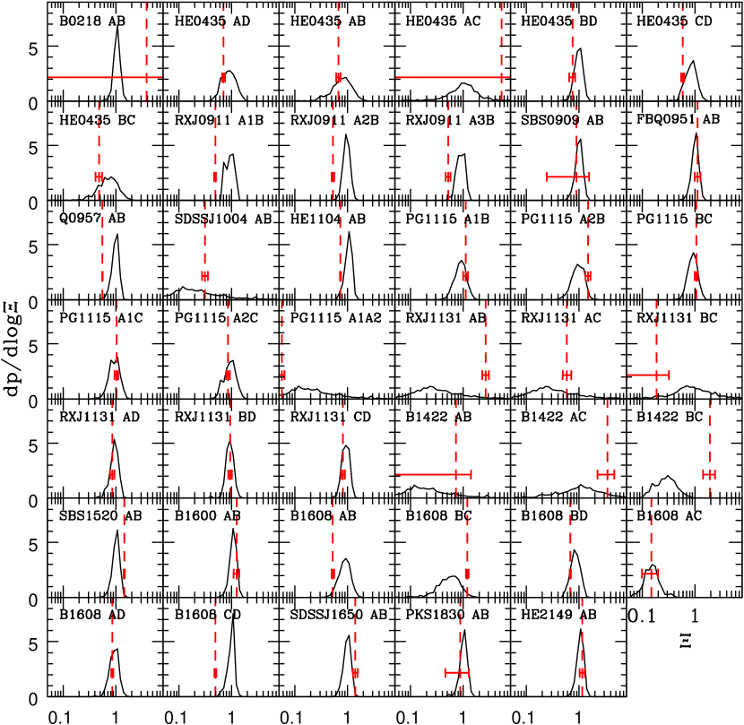
Figure 7.— The conditional probability distributions $p(\Xi|R_{ij},\theta_{ij})$ are compared with reduced time delays $\Xi$ computed from observed time delays of 17 published time delay quasars. Again, the Hubble constant of $h=0.73$ is assumed. Solid line curves are in fact differential probability distribution . In each panel, we draw the differential probability distribution $dp/d\log\Xi$ computed from observed values of $R_{ij}$ and $\theta_{ij}$ by a solid line. Reduced time delays from observed time delays are shown by vertical dashed lines plus error-bars. See Table 4.4 for the summary of observations.

5. Comparison with Observed Time Delays

We now examine if the conditional distribution computed in §4 is consistent with the observed distribution of time delays. Since we need to assume the Hubble constant in order to convert observed time delays to reduce time delays $\Xi$, in this section we adopt $h=0.73$ that was obtained from the combined analysis of the cosmic microwave background (CMB) anisotropy and clustering of galaxies (Tegmark et al., 2006). We derive reduced time delays for the 17 published time delay quasars (41 image pairs), which is summarized in Table 4.4.

First, we compare these reduced time delays with the conditional probability plotted in Figure 4. We show $p(\Xi|R_{ij})$ and $p(\Xi|\theta_{ij})$ with observed values overplotted in Figure 6. It appears that the data are roughly consistent with our probability distribution from simulations. The large scatter of very symmetric lenses is also seen for observed time delays. It is interesting that observed time delays appear to exhibit the decline of time delays at small opening angles, just as our theoretical model predicts. We may need more quasar time delays to confirm this trend observationally.

More directly, observed time delays should be compared with the probability distribution for given $R_{ij}$ and $\theta_{ij}$, i.e., $p(\Xi|R_{ij},\theta_{ij})$. In Figure 7 we compare observed $\Xi$ with the probability distribution of $\Xi$ expected from corresponding image configuration of each image pair. We find that the distributions agree with observed values on average, similarly as Figure 6. The reduced time delays of B0218+357 and SBS0909+532 have larger errors because the positions of the lens galaxies are poorly determined. The large error of HE0435$-$1223 AC comes from small $r_{j}^{2}-r_{i}^{2}$, whereas that of B1422+231 is simply because of the large time delay measurement errors. We comment that RXJ0911+0551 and Q0957+561 has significantly smaller $\Xi$ compared with our model prediction. This is clearly because of the cluster convergence: The two lenses lie in near the centers of clusters and therefore the observed time delays are pushed down by the convergence coming from dark matter in the clusters (see §6). The reduced time delays of B1608+656 and SBS1520+530 are largely offset from the predicted values, and this is probably because of satellite galaxies in the lens systems that significantly affect the time delays. The large time delays of RXJ1131$-$1231 AB and AC were also noted by Morgan et al. (2007): Our result indicates that the broadened theoretical distributions due to small perturbations are enough to explain the observed high values of the time delays. The large offsets of B1422+231 and SDSS J1650+4251 may come from the large uncertainties of measured time delays (see §6).

6. Implications for $H_{0}$

In this section, we turn the problem around and constrain the Hubble constant using the conditional probability distribution constructed from the Monte-Carlo simulations. Although the current sample of observed time delays summarized in Table 4.4 is somewhat heterogeneous and may not be appropriate for the statistical study, we do this to demonstrate how we can constrain the Hubble constant from the probability distribution. We basically take all lens systems listed in Table 4.4, but adopt the following setup to reduce systematic errors.

• We do not use the AB time delay of SDSS J1004+4112. It is a lens system caused by a massive cluster of galaxies, thus our input distribution, which is designed for galaxies, does not represent a fair distribution of lens potentials. Moreover, the center of the lens potential appears to be offset from the position of the brightest cluster galaxy (Oguri et al., 2004), which makes it inaccurate to estimate important parameters such $\Xi$, $R_{ij}$, and $\theta_{ij}$.

• Both RXJ0911+0551 and Q0957+561 are known to reside in the cluster environment, thus they are significantly affected by the cluster convergence $\kappa_{\rm clu}$. Since the mass-sheet degeneracy says $\Xi\propto\Delta t\propto 1-\kappa_{\rm clu}$, we divide reduce time delays $\Xi$ for these two systems by $1-\kappa_{\rm clu}$ in order to deconvolve the effect of the cluster convergence. As the values of $\kappa_{\rm clu}$, we adopt $\kappa_{\rm clu}=0.3\pm 0.04$ for RXJ0911+0551 (Hjorth et al., 2002), and $\kappa_{\rm clu}=0.26\pm 0.08$ for Q0957+561 (Fischer et al., 1997).

In summary, we use 16 lensed quasar systems (40 image pairs) to constrain the Hubble constant. For each image pair, we compute the likelihood as follows:

$$\mathcal{L}_{p}(h)=\int\frac{dp}{d\Xi}(\Xi|R_{ij,{\rm obs}},\theta_{ij,{\rm obs}})G(\Xi|\Xi_{\rm obs}(h))d\Xi,$$ (25)

where $R_{ij,{\rm obs}}$, $\theta_{ij,{\rm obs}}$, $\Xi_{\rm obs}$ are those for this specific image pair listed in Table 4.4, and $G(\Xi|\Xi_{\rm obs}(h))$ indicates the Gaussian distribution with median $\Xi=\Xi_{\rm obs}$. Note that calculating $\Xi_{\rm obs}$ from observed time delays require the Hubble constant $h$, hence $\mathcal{L}_{p}$ is a function of $h$. Then we compute the effective chi-square by summing up the logarithm of the likelihoods:

$$\chi_{\rm eff}(h)=\sum_{\rm quasar}\frac{1}{n_{p}}\sum_{\rm pair}\left[-2\ln\mathcal{L}_{p}(h)\right].$$ (26)

The first summation runs over lens systems, whereas the second summation runs over image pairs for each lens system; the number of pairs for each lens is denoted by $n_{p}$. Note that $n_{p}=1$ all double lens systems, and a quadruple lens system should have $n_{p}\leq{}_{4}{\rm C}_{2}=6$ depending on how many time delays have been observed for the lens system. The factor $1/n_{p}$ was introduced such that all lens systems have equal weight on the effective chi-square irrespective of the number of image pairs. We derive the best-fit value and its error of $h$ by the standard way using a goodness-of-fit parameter $\Delta\chi_{\rm eff}\equiv\chi_{\rm eff}-\chi_{\rm eff}({\rm min})$.

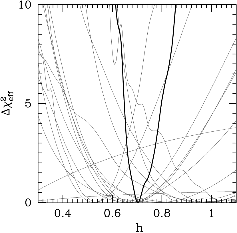
Figure 8.— Statistical constraint on the Hubble constant from 16 time delay quasars (40 image pairs). Thick solid line indicates goodness-of-fit parameter from all 16 lens systems plotted as a function of the Hubble constant $h$. The resulting Hubble constant is $h=0.70^{+0.03}_{-0.02}$ at 68% confidence and $h=0.70^{+0.09}_{-0.05}$ at 95% confidence. The Hubble constant estimated using jackknife resampling has a larger error, $h=0.70\pm 0.06$ at 68% confidence (see text for details). Thin solid lines show goodness-of-fit parameter for each lens system.

We show our result in Figure 8. The Hubble constant measured from the combination of all 16 lens systems is $h=0.70^{+0.03}_{-0.02}$ at 68% confidence and $h=0.70^{+0.09}_{-0.05}$ at 95% confidence. The obtained value is in good agreement with other estimates, such as the local distance measurement using Cepheid calibration (Freedman et al., 2001) and the CMB anisotropy (Tegmark et al., 2006; Spergel et al., 2007). The constraint from each lens system, which is plotted in Figure 8, is summarized in Table 2.

Table 2Hubble Constant from Each Lens System

Lens Name	$h$ ($1\sigma$ range)
B0218+357	0.21 (–)
HE0435$-$1223	1.02 (0.70–1.39)
RXJ0911+0551	0.96 (0.75–1.21)
SBS0909+532	0.84 (0.47–)
FBQ0951+2635	0.67 (0.56–0.81)
Q0957+561	0.99 (0.82–1.17)
HE1104$-$1805	1.04 (0.92–1.22)
PG1115+080	0.66 (0.49–0.84)
RXJ1131$-$1231	0.79 (0.59–1.03)
B1422+231	0.16 (–0.36)
SBS1520+530	0.53 (0.46–0.61)
B1600+434	0.65 (0.54–0.77)
B1608+656	0.89 (0.77–1.20)
SDSS J1650+4251	0.53 (0.44–0.63)
PKS1830$-$211	0.88 (0.58–)
HE2149$-$2745	0.69 (0.57–0.82)
All	0.70 (0.68–0.73)

Note. — The Hubble constant and its error are estimated from the effective chi-square.

We also derive the Hubble constant using the jackknife resampling by regarding each 16 lens system as a subsample. The result $h=0.70\pm 0.06$ at 68% confidence has the same mean but larger error than that estimated from the effective chi-square. There are several possible source of this difference. One is the underestimate of the width of the input distributions. In particular, many of the time delay quasar systems has been claimed to be affected by lens galaxy environments (e.g., Morgan et al., 2005; Fassnacht et al., 2006; Momcheva et al., 2006; Williams et al., 2006; Auger et al., 2007), and thus our input strength of external shear might be somewhat smaller than the true one (see also discussion in §7). Another possible source is the non-Gaussianity of measured time delays: In equation (25) we assumed the Gaussian distribution for the measurement uncertainties of time delays, but sometimes they are quite different from the Gaussian distribution. We note that in our method we can in principle include non-Gaussianity by just replacing $G(\Xi)$ in equation (25) with any appropriate probability distributions, as long as we know such distributions.

7. Discussions and Conclusion

In this paper, we have studied time delays between multiply imaged quasars. Adopting the reduced time delay, which is a measure of how the lens potential is complicated compared with the simple isothermal form, we have explored the dependence of time delays on various complex structure of lens potentials such as external perturbations, non-isothermality, and substructures. The distribution of time delays has been studied as a function of image configuration which we characterize using two dimensionless quantities, the asymmetry and opening angle of an image pair. We have pointed out that the sensitivity on lens potentials is quite dependent on the image configuration. For instance, more symmetric image pairs are more affected by a small change of the lens potential. Image pairs with smaller opening angles are also more sensitive to lens potentials. In particular time delays of close image pairs are very sensitive to higher-order external perturbations and substructures that are very hard to be constrained from mass modeling even for best studied lens systems. In addition, those pairs usually have the largest relative uncertainties of time delay measurements. Therefore we conclude that it is quite difficult to extract any information on the Hubble constant or the mass distribution from close image pairs. It is interesting to note that perturbations on lens potential not only introduce scatter around the mean but also can systematically shift the distribution of time delays. One such example is smaller time delays for smaller opening angle image pairs, which is caused by external shear.

We have performed Monte-Carlo simulations to derive a probability distribution of reduced time delays for each image configuration. Input distributions are determined from observational and theoretical constraints. The distribution is weighted by the lensing cross section and magnification bias, allowing a realistic estimate of time delay distributions. The probability distribution was then compared with observed time delays. We have shown that the distribution of time delays computed from our simulations is in good agreement with observed time delays. In particular, distributions of observed time delays also exhibit strong dependence of image configuration in a consistent manner with our theoretical expectations. The probability distribution can be used to constrain the Hubble constant. We have found that 16 published time delay quasars constrain it to be $h=0.70^{+0.03}_{-0.02}$ at 68% confidence using the effective chi-square or $h=0.70\pm 0.06$ estimated using jackknife resampling, consistent with other estimates.

An important caveat is that our lensed quasar sample is quite heterogeneous. In particular, it should be noted that current time delay quasars (see Table 4.4) have significantly larger image separations on average compared with the other quasar lenses: The median image separation of time delay quasars listed in Table 4.4 is $1\farcs 7$ (image separations before and after the median are $1\farcs 5$ and $2\farcs 1$), whereas that of all lensed quasars is $\sim 1\farcs 4$. Quasar lenses with larger image separations are more likely to lie in dense environments because both the image separation and biased cross section are boosted by surrounding dark matter (Oguri et al., 2005; Oguri, 2006), thus the Hubble constant inferred from those lenses are more affected by the environmental convergence. Indeed, the association of group/cluster has been reported for more than half of the time delay quasars (e.g., Morgan et al., 2005; Fassnacht et al., 2006; Momcheva et al., 2006; Williams et al., 2006; Auger et al., 2007). In addition, our input distributions of external perturbations may be underestimated for these large separation lenses. To estimate this systematic effect, we exclude four lensed quasars with image separation larger than $3^{\prime\prime}$ and repeat the analysis done in §6. The resulting Hubble constant $h=0.67^{+0.04}_{-0.03}$ at 68% confidence from the effective chi-square is consistent with our full result, thus we conclude that the effect of lens galaxy environments is not so drastic here. However, to minimize the systematic effect, in the future we should apply our statistical method to well-defined samples of lensed quasars such as the CLASS (Myers et al., 2003; Browne et al., 2003), SQLS (Oguri et al., 2006), and those obtained in future lens surveys.

Another source of the systematic effect is the uncertainty of our input distribution of lens potentials. Among others, the most important systematic error comes from the uncertainty of the mean value of the slope of the radial profile, $\alpha$. While $\alpha=1$ (isothermal) for the mean appears to be a reasonable choice, direct studies of lens galaxies (e.g., Treu & Koopmans, 2004; Rusin & Kochanek, 2005; Hamana et al., 2007) indicate that the error on the mean $\alpha$ could be as large as 0.1. The derived Hubble constant depends on the slope as $h\propto 2-\alpha$, therefore the change of the mean $\alpha$ systematically shifts the best-fit value. The scaling relation suggests that the 0.1 error of the mean results in 10% error on $h$, indicating that the systematic error may be even larger than the statistical error. Another important systematic effect is caused by external convergence from lens galaxy environments. Since its effect on the Hubble constant is straightforward (e.g., Keeton & Zabludoff, 2004), one can estimate the effect of external convergence rather easily even without including the distribution in the simulation. From the result of Oguri et al. (2005), we expect that the posterior distribution of external convergence with lensing bias taken into account is roughly $\kappa_{\rm ext}\sim 0.03\pm 0.03$ unless the image separation is too large. This, combined with the fact that the Hubble constant scales as $h\propto 1-\kappa_{\rm ext}$, suggest that the effect of external convergence is not so dominant here (note that external convergence was already taken into account for two extreme lenses, Q0957+561 and RXJ0911+0551). By including rough estimates of these two systematic errors, we obtain $h=0.68\pm 0.06({\rm stat.})\pm 0.08({\rm syst.})$, indicating the importance of reducing the systematic error.

Since the Hubble constant is now determined fairly well by other methods, time delays are sometimes used to study mass distributions of lens objects. Our statistical technique offers a new method to study the lens mass distribution. By comparing the probability distributions for different input distributions of lens potentials (e.g., different median slopes of the primary lens galaxy), one can infer which input model is most plausible. Unlike previous statistical studies (e.g., Oguri et al., 2002), this new method allows us to include various complexity of lens potentials relatively easily, particularly the non-spherically symmetric nature of lens potentials. We note that our input distribution of lens potentials was designed for galaxies, but it is straightforward to modify it to that of lensing by other populations, e.g., lensing by a cluster of galaxies.

In summary, our new statistical approach is invaluable for the study of both cosmological parameters and structure of lens potentials. We believe its importance grows more and more in the era of large-scale synoptic surveys such as LSST and SNAP: Quasar lens candidates are easily recognized in these synoptic surveys by making use of strong time variability of quasars (Pindor, 2005; Kochanek et al., 2006a). Strong lensing of distant supernovae offers additional interesting opportunity to apply our statistical technique. The statistical analysis is essential to make efficient use of the large homogeneous samples of strong lenses provided by these surveys.

References

- Auger et al. (2007) Auger, M. W., Fassnacht, C. D., Abrahamse, A. L., Lubin, L. M., & Squires, G. K. 2007, AJ, submitted (astro-ph/0603448)
- Bade et al. (1997) Bade, N., Siebert, J., Lopez, S., Voges, W., & Reimers, D. 1997, A&A, 317, L13
- Barkana (1997) Barkana, R. 1997, ApJ, 489, 21
- Barkana et al. (1999) Barkana, R., Lehár, J., Falco, E. E., Grogin, N. A., Keeton, C. R., & Shapiro, I. I. 1999, ApJ, 520, 479
- Bernstein & Fischer (1999) Bernstein, G., & Fischer, P. 1999, AJ, 118, 14
- Biggs et al. (1999) Biggs, A. D., Browne, I. W. A., Helbig, P., Koopmans, L. V. E., Wilkinson, P. N., & Perley, R. A. 1999, MNRAS, 304, 349
- Bender et al. (1989) Bender, R., Surma, P., Doebereiner, S., Moellenhoff, C., & Madejsky, R. 1989, A&A, 217, 35
- Blandford & Narayan (1986) Blandford, R., & Narayan, R. 1986, ApJ, 310, 568
- Bradač et al. (2002) Bradač, M., Schneider, P., Steinmetz, M., Lombardi, M., King, L. J., & Porcas, R. 2002, A&A, 388, 373
- Browne et al. (1993) Browne, I. W. A., Patnaik, A. R., Walsh, D., & Wilkinson, P. N. 1993, MNRAS, 263, L32
- Browne et al. (2003) Browne, I. W. A., et al. 2003, MNRAS, 341, 13
- Burud et al. (2000) Burud, I., et al. 2000, ApJ, 544, 117
- Burud et al. (2002a) Burud, I., et al. 2002a, A&A, 383, 71
- Burud et al. (2002b) Burud, I., et al. 2002b, A&A, 391, 481
- Chavushyan et al. (1997) Chavushyan, V. H., Vlasyuk, V. V., Stepanian, J. A., & Erastova, L. K. 1997, A&A, 318, L67
- Chen et al. (2003) Chen, J., Kravtsov, A. V., & Keeton, C. R. 2003, ApJ, 592, 24
- Chartas et al. (2004) Chartas, G., Dai, X., & Garmire, G. P. 2004, in the Carnegie Observatories Centennial Symposia Carnegie Observatories Astrophysics Series, Measuring and Modeling the Universe, ed. W. L. Freedman (Pasadena: Carnegie Observatories), http://www.ociw.edu/ociw/symposia/series/symposium2/proceedings.html
- Chiba (2002) Chiba, M. 2002, ApJ, 565, 17
- Chiba et al. (2005) Chiba, M., Minezaki, T., Kashikawa, N., Kataza, H., & Inoue, K. T. 2005, ApJ, 627, 53
- Cohen et al. (2003) Cohen, J. G., Lawrence, C. R., & Blandford, R. D. 2003, ApJ, 583, 67
- Cohn et al. (2001) Cohn, J. D., Kochanek, C. S., McLeod, B. A., & Keeton, C. R. 2001, ApJ, 554, 1216
- Congdon & Keeton (2005) Congdon, A. B., & Keeton, C. R. 2005, MNRAS, 364, 1459
- Dai et al. (2003) Dai, X., Chartas, G., Agol, E., Bautz, M. W., & Garmire, G. P. 2003, ApJ, 589, 100
- Dalal & Kochanek (2002) Dalal, N., & Kochanek, C. S. 2002, ApJ, 572, 25
- Dalal & Watson (2004) Dalal, N., & Watson, C. R. 2004, astro-ph/0409483
- De Lucia et al. (2004) De Lucia, G., Kauffmann, G., Springel, V., White, S. D. M., Lanzoni, B., Stoehr, F., Tormen, G., & Yoshida, N. 2004, MNRAS, 348, 333
- Dobke & King (2006) Dobke, B. M., & King, L. J. 2006, A&A, 460, 647
- Dobler & Keeton (2006) Dobler, G., & Keeton, C. R. 2006, ApJ, 653, 1391
- Eigenbrod et al. (2007) Eigenbrod, A., Courbin, F., & Meylan, G. 2007, A&A, in press (astro-ph/0612419)
- Falco et al. (1985) Falco, E. E., Gorenstein, M. V., & Shapiro, I. I. 1985, ApJ, 289, L1
- Fassnacht et al. (2006) Fassnacht, C. D., Gal, R. R., Lubin, L. M., McKean, J. P., Squires, G. K., & Readhead, A. C. S. 2006, ApJ, 642, 30
- Fassnacht et al. (1996) Fassnacht, C. D., Womble, D. S., Neugebauer, G., Browne, I. W. A., Readhead, A. C. S., Matthews, K., & Pearson, T. J. 1996, ApJ, 460, L103
- Fassnacht & Cohen (1998) Fassnacht, C. D., & Cohen, J. G. 1998, AJ, 115, 377
- Fassnacht et al. (2002) Fassnacht, C. D., Xanthopoulos, E., Koopmans, L. V. E., & Rusin, D. 2002, ApJ, 581, 823
- Faure et al. (2002) Faure, C., Courbin, F., Kneib, J. P., Alloin, D., Bolzonella, M., & Burud, I. 2002, A&A, 386, 69
- Fischer et al. (1997) Fischer, P., Bernstein, G., Rhee, G., & Tyson, J. A. 1997, AJ, 113, 521
- Fohlmeister et al. (2007) Fohlmeister, J., et al. 2007, ApJ, submitted (astro-ph/0607513)
- Freedman et al. (2001) Freedman, W. L., et al. 2001, ApJ, 553, 47
- Hamana et al. (2007) Hamana, T., Ohyama, Y., Chiba, M., & Kashikawa, N. 2007, MNRAS, submitted (astro-ph/0507056)
- Hjorth et al. (2002) Hjorth, J., et al. 2002, ApJ, 572, L11
- Holder & Schechter (2003) Holder, G. P., & Schechter, P. L. 2003, ApJ, 589, 688
- Impey et al. (1998) Impey, C. D., Falco, E. E., Kochanek, C. S., Lehár, J., McLeod, B. A., Rix, H.-W., Peng, C. Y., & Keeton, C. R. 1998, ApJ, 509, 551
- Inada et al. (2003) Inada, N., et al. 2003, Nature, 426, 810
- Inada et al. (2005) Inada, N., et al. 2005, PASJ, 57, L7
- Jackson et al. (1995) Jackson, N., et al. 1995, MNRAS, 274, L25
- Jakobsson et al. (2005) Jakobsson, P., Hjorth, J., Burud, I., Letawe, G., Lidman, C., & Courbin, F. 2005, A&A, 431, 103
- Jorgensen et al. (1995) Jorgensen, I., Franx, M., & Kjaergaard, P. 1995, MNRAS, 273, 1097
- Kawano et al. (2004) Kawano, Y., Oguri, M., Matsubara, T., & Ikeuchi, S. 2004, PASJ, 56, 253
- Kawano & Oguri (2006) Kawano, Y., & Oguri, M. 2006, PASJ, 58, 271
- Keeton (2001) Keeton, C. R. 2001, astro-ph/0102340
- Keeton (2003) Keeton, C. R. 2003, ApJ, 584, 664
- Keeton et al. (2003) Keeton, C. R., Gaudi, B. S., & Petters, A. O. 2003, ApJ, 598, 138
- Keeton et al. (2005) Keeton, C. R., Gaudi, B. S., & Petters, A. O. 2005, ApJ, 635, 35
- Keeton & Kochanek (1997) Keeton, C. R., & Kochanek, C. S. 1997, ApJ, 487, 42
- Keeton et al. (1997) Keeton, C. R., Kochanek, C. S., & Seljak, U. 1997, ApJ, 482, 604
- Keeton & Zabludoff (2004) Keeton, C. R., & Zabludoff, A. I. 2004, ApJ, 612, 660
- Keeton et al. (2000) Keeton, C. R., et al. 2000, ApJ, 542, 74
- Klypin et al. (1999) Klypin, A., Kravtsov, A. V., Valenzuela, O., & Prada, F. 1999, ApJ, 522, 82
- Kneib et al. (2000) Kneib, J.-P., Cohen, J. G., & Hjorth, J. 2000, ApJ, 544, L35
- Kochanek (1991) Kochanek, C. S. 1991, ApJ, 373, 354
- Kochanek (2002) Kochanek, C. S. 2002, ApJ, 578, 25
- Kochanek (2003) Kochanek, C. S. 2003, ApJ, 583, 49
- Kochanek et al. (2006a) Kochanek, C. S., Mochejska, B., Morgan, N. D., & Stanek, K. Z. 2006a, ApJ, 637, L73
- Kochanek (2006) Kochanek, C. S., Schneider, P., Wambsganss, J., 2006, Part 2 of Gravitational Lensing: Strong, Weak & Micro, Proceedings of the 33rd Saas-Fee Advanced Course, G. Meylan, P. Jetzer & P. North, eds. (Springer-Verlag: Berlin), 91
- Kochanek & Dalal (2004) Kochanek, C. S., & Dalal, N. 2004, ApJ, 610, 69
- Kochanek et al. (2001) Kochanek, C. S., Keeton, C. R., & McLeod, B. A. 2001, ApJ, 547, 50
- Kochanek et al. (2006b) Kochanek, C. S., Morgan, N. D., Falco, E. E., McLeod, B. A., Winn, J. N., Dembicky, J., & Ketzeback, B. 2006b, ApJ, 640, 47
- Koopmans et al. (1998) Koopmans, L. V. E., de Bruyn, A. G., & Jackson, N. 1998, MNRAS, 295, 534
- Koopmans & Fassnacht (1999) Koopmans, L. V. E., & Fassnacht, C. D. 1999, ApJ, 527, 513
- Koopmans et al. (2006) Koopmans, L. V. E., Treu, T., Bolton, A. S., Burles, S., & Moustakas, L. A. 2006, ApJ, 649, 599
- Koopmans et al. (2003) Koopmans, L. V. E., Treu, T., Fassnacht, C. D., Blandford, R. D., & Surpi, G. 2003, ApJ, 599, 70
- Kundic et al. (1997) Kundic, T., et al. 1997, ApJ, 482, 75
- Lehár et al. (2000) Lehár, J., et al. 2000, ApJ, 536, 584
- Lidman et al. (1999) Lidman, C., Courbin, F., Meylan, G., Broadhurst, T., Frye, B., & Welch, W. J. W. 1999, ApJ, 514, L57
- Lidman et al. (2000) Lidman, C., Courbin, F., Kneib, J.-P., Golse, G., Castander, F., & Soucail, G. 2000, A&A, 364, L62
- Lovell et al. (1998) Lovell, J. E. J., Jauncey, D. L., Reynolds, J. E., Wieringa, M. H., King, E. A., Tzioumis, A. K., McCulloch, P. M., & Edwards, P. G. 1998, ApJ, 508, L51
- Lubin et al. (2000) Lubin, L. M., Fassnacht, C. D., Readhead, A. C. S., Blandford, R. D., & Kundić, T. 2000, AJ, 119, 451
- Mao et al. (2004) Mao, S., Jing, Y., Ostriker, J. P., & Weller, J. 2004, ApJ, 604, L5
- Metcalf (2005) Metcalf, R. B. 2005, ApJ, 629, 673
- Metcalf & Madau (2001) Metcalf, R. B., & Madau, P. 2001, ApJ, 563, 9
- Metcalf et al. (2004) Metcalf, R. B., Moustakas, L. A., Bunker, A. J., & Parry, I. R. 2004, ApJ, 607, 43
- Möller et al. (2007) Möller, O., Kitzbichler, M., & Natarajan, P. 2007, MNRAS, submitted (astro-ph/0607032)
- Momcheva et al. (2006) Momcheva, I., Williams, K., Keeton, C., & Zabludoff, A. 2006, ApJ, 641, 169
- Moore et al. (1999) Moore, B., Ghigna, S., Governato, F., Lake, G., Quinn, T., Stadel, J., & Tozzi, P. 1999, ApJ, 524, L19
- Morgan et al. (2003) Morgan, N. D., Snyder, J. A., & Reens, L. H. 2003, AJ, 126, 2145
- Morgan et al. (2005) Morgan, N. D., Kochanek, C. S., Pevunova, O., & Schechter, P. L. 2005, AJ, 129, 2531
- Morgan et al. (2007) Morgan, N. D., Kochanek, C. S., Falco, E. E., & Dai, X. 2007, ApJ, submitted (astro-ph/0605321)
- Mörtsell et al. (2005) Mörtsell, E., Dahle, H., & Hannestad, S. 2005, ApJ, 619, 733
- Myers et al. (1995) Myers, S. T., et al. 1995, ApJ, 447, L5
- Myers et al. (2003) Myers, S. T., et al. 2003, MNRAS, 341, 1
- Ofek & Maoz (2003) Ofek, E. O., & Maoz, D. 2003, ApJ, 594, 101
- Oguri (2005) Oguri, M. 2005, MNRAS, 361, L38
- Oguri (2006) Oguri, M. 2006, MNRAS, 367, 1241
- Oguri & Kawano (2003) Oguri, M., & Kawano, Y. 2003, MNRAS, 338, L25
- Oguri et al. (2005) Oguri, M., Keeton, C. R., & Dalal, N. 2005, MNRAS, 364, 1451
- Oguri & Lee (2004) Oguri, M., & Lee, J. 2004, MNRAS, 355, 120
- Oguri et al. (2003) Oguri, M., Suto, Y., & Turner, E. L. 2003, ApJ, 583, 584
- Oguri et al. (2002) Oguri, M., Taruya, A., Suto, Y., & Turner, E. L. 2002, ApJ, 568, 488
- Oguri et al. (2004) Oguri, M., et al. 2004, ApJ, 605, 78
- Oguri et al. (2006) Oguri, M., et al. 2006, AJ, 132, 999
- Oscoz et al. (1997) Oscoz, A., Serra-Ricart, M., Mediavilla, E., Buitrago, J., & Goicoechea, L. J. 1997, ApJ, 491, L7
- Patnaik et al. (1992) Patnaik, A. R., Browne, I. W. A., Walsh, D., Chaffee, F. H., & Foltz, C. B. 1992, MNRAS, 259, 1P
- Patnaik et al. (1993) Patnaik, A. R., Browne, I. W. A., King, L. J., Muxlow, T. W. B., Walsh, D., & Wilkinson, P. N. 1993, MNRAS, 261, 435
- Patnaik & Narasimha (2001) Patnaik, A. R., & Narasimha, D. 2001, MNRAS, 326, 1403
- Pindor (2005) Pindor, B. 2005, ApJ, 626, 649
- Poindexter et al. (2006) Poindexter, S., Morgan, N., Kochanek, C. S., & Falco, E. E. 2006, ApJ, submitted (astro-ph/0612045)
- Refsdal (1964) Refsdal, S. 1964, MNRAS, 128, 307
- Refsdal & Surdej (1994) Refsdal, S., & Surdej, J. 1994, Rep. Prog. Phys., 57, 117
- Rest et al. (2001) Rest, A., van den Bosch, F. C., Jaffe, W., Tran, H., Tsvetanov, Z., Ford, H. C., Davies, J., & Schafer, J. 2001, AJ, 121, 2431
- Rusin & Kochanek (2005) Rusin, D., & Kochanek, C. S. 2005, ApJ, 623, 666
- Rusin et al. (2003) Rusin, D., Kochanek, C. S., & Keeton, C. R. 2003, ApJ, 595, 29
- Saglia et al. (1993) Saglia, R. P., Bender, R., & Dressler, A. 1993, A&A, 279, 75
- Saha (2000) Saha, P. 2000, AJ, 120, 1654
- Saha (2004) Saha, P. 2004, A&A, 414, 425
- Saha et al. (2006) Saha, P., Coles, J., Maccio’, A. V., & Williams, L. L. R. 2006, ApJ, 650, L17
- Saha & Williams (2006) Saha, P., & Williams, L. L. R. 2006, ApJ, 653, 936
- Schechter (2005) Schechter, P. L. 2005, IAU Symposium, 225, 281
- Schechter et al. (1998) Schechter, P. L., Gregg, M. D., Becker, R. H., Helfand, D. J., & White, R. L. 1998, AJ, 115, 1371
- Schechter et al. (1997) Schechter, P. L., et al. 1997, ApJ, 475, L85
- Sheth et al. (2003) Sheth, R. K., et al. 2003, ApJ, 594, 225
- Sluse et al. (2003) Sluse, D., et al. 2003, A&A, 406, L43
- Spergel et al. (2007) Spergel, D. N., et al. 2007, ApJ, submitted (astro-ph/0603449)
- Subrahmanyan et al. (1990) Subrahmanyan, R., Narasimha, D., Pramesh-Rao, A., & Swarup, G. 1990, MNRAS, 246, 263
- Tada & Futamase (2000) Tada, M., & Futamase, T. 2000, Prog. Theor. Phys., 104, 971
- Tegmark et al. (2006) Tegmark, M., et al. 2006, Phys. Rev. D, 74, 123507
- Tonry (1998) Tonry, J. L. 1998, AJ, 115, 1
- Treu & Koopmans (2002) Treu, T., & Koopmans, L. V. E. 2002, MNRAS, 337, L6
- Treu & Koopmans (2004) Treu, T., & Koopmans, L. V. E. 2004, ApJ, 611, 739
- Trotter et al. (2000) Trotter, C. S., Winn, J. N., & Hewitt, J. N. 2000, ApJ, 535, 671
- Turner et al. (1984) Turner, E. L., Ostriker, J. P., & Gott, J. R., III 1984, ApJ, 284, 1
- Ullán et al. (2006) Ullán, A., Goicoechea, L. J., Zheleznyak, A. P., Koptelova, E., Bruevich, V. V., Akhunov, T., & Burkhonov, O. 2006, A&A, 452, 25
- Vakulik et al. (2006) Vakulik, V., Schild, R., Dudinov, V., Nuritdinov, S., Tsvetkova, V., Burkhonov, O., & Akhunov, T. 2006, A&A, 447, 905
- Vuissoz et al. (2007) Vuissoz, C., et al. 2007, A&A, in press (astro-ph/0606317)
- Walsh et al. (1979) Walsh, D., Carswell, R. F., & Weymann, R. J. 1979, Nature, 279, 381
- Weymann et al. (1980) Weymann, R. J., et al. 1980, Nature, 285, 641
- Wiklind & Combes (1996) Wiklind, T., & Combes, F. 1996, Nature, 379, 139
- Williams et al. (2006) Williams, K. A., Momcheva, I., Keeton, C. R., Zabludoff, A. I., & Lehár, J. 2006, ApJ, 646, 85
- Winn et al. (2004) Winn, J. N., Rusin, D., & Kochanek, C. S. 2004, Nature, 427, 613
- Wisotzki et al. (1993) Wisotzki, L., Koehler, T., Kayser, R., & Reimers, D. 1993, A&A, 278, L15
- Wisotzki et al. (1996) Wisotzki, L., Koehler, T., Lopez, S., & Reimers, D. 1996, A&A, 315, L405
- Wisotzki et al. (2002) Wisotzki, L., Schechter, P. L., Bradt, H. V., Heinmüller, J., & Reimers, D. 2002, A&A, 395, 17
- Witt et al. (1995) Witt, H. J., Mao, S., & Schechter, P. L. 1995, ApJ, 443, 18
- Witt et al. (2000) Witt, H. J., Mao, S., & Keeton, C. R. 2000, ApJ, 544, 98
- Wucknitz (2002) Wucknitz, O. 2002, MNRAS, 332, 951
- Wucknitz et al. (2004) Wucknitz, O., Biggs, A. D., & Browne, I. W. A. 2004, MNRAS, 349, 14
- Yoo et al. (2006) Yoo, J., Kochanek, C. S., Falco, E. E., & McLeod, B. A. 2006, ApJ, 642, 22
- Young et al. (1981) Young, P., Gunn, J. E., Oke, J. B., Westphal, J. A., & Kristian, J. 1981, ApJ, 244, 736
- Zhao & Qin (2003) Zhao, H., & Qin, B. 2003, ApJ, 582, 2