Reconstructing the Thomson Optical Depth due to Patchy Reionization with 21-cm Fluctuation Maps

Abstract

Large fluctuations in the electron column density can occur during the reionization process. We investigate the possibility of deriving the electron density fluctuations through detailed mapping of the redshifted 21-cm emission from the neutral medium during reionization. We find that the electron-scattering optical depth and 21-cm differential brightness temperature are strongly anti-correlated, allowing optical depth estimates based entirely on redshifted 21-cm measurements. This should help to isolate the cosmic microwave background (CMB) polarization fluctuations due to reionization, allowing the removal of the patchy reionization polarization signal from the other polarization signals and a measurement of the primordial CMB quadrupole at various locations in the universe at the epoch of reionization. This latter application in principle allows three-dimensional mapping of the primordial density field at $z\sim 1100$ over a large fraction of the Hubble volume.

1. Introduction

Two new frontiers in astrophysics and cosmology are the search for small angle polarization anisotropies in the cosmic microwave background and the efforts to map the redshifted 21-cm emission from neutral hydrogen at the epoch of reionization. On small angular scales, a significant source of CMB polarization comes from Thomson scattering of the primordial quadrupole anisotropy by compact regions of ionized gas. These ionized regions would appear in maps of the neutral gas as holes in a relatively uniform map. Thus we expect that where there are strong sources of Thomson scattering there should be missing 21-cm emission and where there is strong 21-cm emission there should be low Thomson optical depth, $\tau_{\rm es}$, i.e. the two should be anti-correlated. In this paper we investigate the relation between $\tau_{\rm es}$ and neutral hydrogen optical depth in a quantitative way that properly captures the relevant physics using numerical simulations of structure formation with radiative transfer.

This topic is also related to the idea of Kamionkowski & Loeb (1997) for using polarized CMB anisotropy due to Thomson scattering by galaxy clusters of the CMB temperature quadrupole as a means to extract more information about the density field at $z\sim 1100$ than we can measure in the CMB (Sazonov & Sunyaev, 1999; Seto & Sasaki, 2000; Baumann & Cooray, 2003; Portsmouth, 2004; Seto & Pierpaoli, 2005; Bunn, 2006; Shimon et al., 2006). The information content of the quadrupole measurements has been carefully investigated by Bunn (2006) , where it was found that higher redshift clusters are preferred for this, since there is less overlap with our measured CMB sky. Cluster $\tau_{\rm es}$ are typically around 0.005 (Mason & Myers, 2000), and we will show that typical fluctuations of $\tau_{\rm es}$ during reionization can be of comparable size. The quadrupole at the time of reionization should not be affected by the integrated Sachs-Wolfe effect and thus provides a remarkably clean measure of very large scale structure at $z\sim 1100$.

Reionization occurs in a patchy way: strongly-clustered sources create large ionized regions embedded in a mainly neutral medium, which generates CMB polarization anisotropies on small scales. Scattering of the primordial CMB temperature quadrupole leads to linearly polarized signals from ionized regions, where the size of the ionized bubble sets the scale of the anisotropy. On large scales, the relevant quantity is just the mean ionization as a function of redshift, since the small scale structure is averaged out. This is the signal that WMAP detected as the hallmark of reionization.

The amplitude of the expected signal is expected to be on the order of the fluctuations in the electron scattering optical depth times the amplitude of the relevant primordial quadrupole. The latter should be on the order of 15 $\mu K$ but the former is not well constrained at present. Calculations done assuming that the ionization fluctuations can be treated as a Gaussian random field find very small fluctuations, since modes along the line of sight (LOS) tend to average down (Hu, 2000). However, recent simulations (Iliev et al., 2006b; Mellema et al., 2006b) show surprisingly large fluctuations in the optical depth, on the order of 0.01 coming just from the epoch of reionization, as we will show below. This optical depth is larger than that found in even the largest galaxy clusters in the local universe. The all-or-nothing nature of the ionized regions effectively breaks the Limber approximation, often leading to very little cancellation along the LOS. Recent work has suggested that patchy reionization scenarios can result in interesting levels of CMB polarization (Mortonson & Hu, 2006).

In principle, one can use a H I map to synthesize an effective $\tau_{\rm es}$ map and compare with a CMB polarization map to infer the CMB quadrupole at the location of the scattering. Naively, the fluctuation maps (after subtraction of the spatial means) should differ only by an overall amplitude scaling, provided the primordial quadrupole is slowly varying over the epoch of reionization.

We assume a flat $\Lambda$CDM cosmology with parameters ($\Omega_{m},\Omega_{\Lambda},\Omega_{b},h,\sigma_{8},n)=(0.27,0.73,0.044,0.7,0.9,1)$ (Spergel, 2003), where $\Omega_{m}$, $\Omega_{\Lambda}$, and $\Omega_{b}$ are the total matter, vacuum, and baryonic densities in units of the critical density, $\sigma_{8}$ is the present rms linear density fluctuation on the scale of $8h^{-1}{\rm Mpc}$, and $n$ is the index of the primordial power spectrum of density fluctuations.

2. Simulations

Our basic methodology was described in detail in Iliev et al. (2006b). We start by performing a high resolution $100\,h^{-1}$Mpc N-body simulation with a spatial grid of $3248^{3}$ cells, $1624^{3}=4.3$ billion particles, and using the particle-mesh code PMFAST (Merz et al., 2005). This yields detailed halo catalogues, and density and velocity fields at up to 100 roughly equally-spaced times. All halos identified in our simulation volume are assumed to be sources of ionizing radiation with ionizing photon emissivity given by a constant mass-to-light ratio. We follow the time-dependent propagation of the ionization fronts produced by sources in the simulation volume using a detailed radiative transfer and non-equilibrium chemistry code called $C^{2}$-Ray (Mellema et al., 2006a), which has been extensively tested against available analytical solutions (Mellema et al., 2006a) and a number of other cosmological radiative transfer codes (Iliev et al., 2006a). The transport of ionizing radiation is done on a coarsened grid of $203^{3}$ or $406^{3}$ cells, in order to make the problem tractable. These simulations allow for a number of detailed predictions of 21-cm (Mellema et al., 2006b) and kSZ signals (Iliev et al., 2006c, ; Iliev et al. in prep.). In this work we use data from simulation f2000 (see Mellema et al., 2006b), though our conclusions are generic.

3. Fluctuations from Patchy Reionization

3.1. 21-cm Emission Fluctuations

For our assumed cosmology (where dark energy and curvature are dynamically unimportant at the epoch of reionization) and ignoring the peculiar motions (i.e. assuming that the line profile is determined solely by the Hubble expansion) the 21-cm optical depth of a hydrogen cloud can be written as

$$\tau(\nu) = \frac{3hc^{3}A_{10}}{32\pi k_{B}T_{S}\nu_{0}^{2}}\frac{n_{\rm HI}(z)}{H(z)}$$ (1)

$$= {8.5mK\over T_{S}}x_{\rm HI}(1+\delta_{\rho})(1+z)^{3/2},$$

where $A_{10}=2.85\times 10^{-15}$ is the Einstein A-coefficient for spin-flip transition, $T_{S}$ is the 21-cm transition spin temperature, $\nu_{0}$ is the rest-frame line frequency, $H(z)=H_{0}{\Omega_{m}}^{1/2}(1+z)^{3/2}$ is the Hubble constant at redshift $z$, and $n_{\rm HI}(z)$ is the hydrogen number density, $x_{\rm HI}$ is the mass-weighted neutral fraction of hydrogen and $\delta_{\rho}$ is the local overdensity (e.g. Iliev et al., 2002). For simplicity, we assume that the spin temperature is much greater than the CMB temperature, which should be a good approximation after the earliest phases of reionization, and that $\tau\ll 1$, in which case the 21-cm differential brightness temperature is given by:

$$\Delta T_{b}(\nu) = {T_{S}-T_{\rm cmb}\over 1+z}[1-e^{-\tau(\nu)}]$$ (2)

$$\approx 8.5\,mK\,x_{HI}\left(1+{\delta_{\rho}}\right)(1+z)^{1/2}.$$

We can express the neutral fraction in terms of the mean ionized fraction and fluctuations around the mean

$$x_{\rm HI}\equiv 1-\bar{x}_{m}-\delta x,$$ (3)

where $\bar{x}_{m}$ is the mean mass-weighted ionized fraction and $\delta x$ is the fluctuation in the ionized hydrogen fraction. Combining equations (2) and (3) yields

$$\Delta T_{b}(\nu) \approx 8.5\,mK(1+z)^{1/2}$$ (4)

$$\times [1-\bar{x}_{m}+(1-\bar{x}_{m})\delta_{\rho}-\delta x(1+\delta_{\rho})].$$

If we subtract off the spatial mean, as most observing schemes necessarily would, then the fluctuations in the 21-cm emission are given by

$$\delta[\Delta T_{b}(\nu)] \approx 8.5\,mK(1+z)^{1/2}$$ (5)

$$\times [(1-\bar{x}_{m})\delta_{\rho}-\delta x(1+\delta_{\rho})].$$

3.2. Thomson optical depth fluctuations

The optical depth to Thomson scattering is

$$\tau_{\rm es}=\int n_{e}(z)\,\sigma_{T}\,c\,dt,$$ (6)

where $\sigma_{T}$ is the Thomson cross-section. There is some subtlety here in relating this to the hydrogen distribution, since some of the free electrons come from ionized helium. For simplicity we assume that fluctuations in the helium ionization trace the hydrogen ionization. Extreme variations in the ionization state of helium could change the optical depth fractionally at the 10% level. Using $N_{\rm He}$ to denote the number of electrons from helium ionizations per hydrogen ionization

$$\tau_{\rm es} = \int(1+N_{\rm He})n_{H}(0)(1+z)^{2}\sigma_{T}\,{c\over H(z)}$$ (7)

$$\times [\bar{x}_{m}(1+\delta_{\rho})+\delta x(1+{\delta_{\rho}})]dz.$$

Subtracting the spatially uniform part we find

$$\delta\tau_{\rm es} = 0.0031(1+N_{\rm He})$$ (8)

$$\times \int dz[\bar{x}_{m}{\delta_{\rho}}+\delta x(1+{\delta_{\rho}})](1+z)^{1/2}.$$

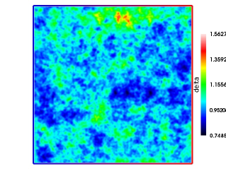
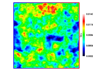
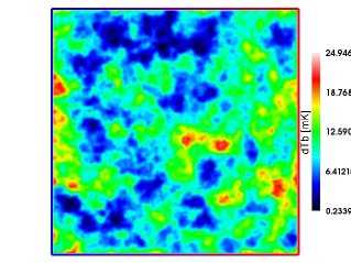
Figure 1.— Maps of a single redshift output (z=12.9) showing integrated overdensity (left) integrated Thomson optical depth (middle) and integrated 21-cm emission (right) through the computational volume ($6.6$ MHz bandwidth). Each map is 47.5’ on a side, with each pixel about 14”. (Maps were produced using the package IFRIT of N. Gnedin).

Figure 2.— Contour plots from maps constructed from single redshift output showing integrated optical depth vs 21-cm integrated intensity. Shown is the distribution of map pixels, with contours showing a density of points that is 1, 10, and 100 points per cell. From left to right shows redshift 11.9, 12.6 and 13.6. The heavy line shows the expectation in the absence of fluctuations in the projected density map. Scatter comes from density fluctuations, while the change in slope (shown by the thin line) arises due to density-ionization correlations.

4. Combining data sets

Sample maps with bandwidth of $\sim 6.6$ MHz (corresponding to the whole computational volume) of the integrated overdensity, Thomson optical depth, and 21-cm differential brightness temperature fluctuations are shown in Figure 2. If the perturbations were small, linear and Gaussian, $\delta\tau_{\rm es}$ would be small. From the maps it is apparent that this is not the case. The large-bandwidth 21-cm map is an excellent negative image of the optical depth map, indicating that 21-cm imaging can in fact be used for inferring the optical depth fluctuations. Comparing equations (5) and (8) we find

$$\delta\tau_{\rm es}=0.0031(1+N_{\rm He})\int\Bigl{(}{\delta_{\rho}}(1+z)^{1/2}-\frac{\delta\left\{\Delta T[\nu(z)]\right\}}{8.5\,\rm mK}\Bigr{)}dz.$$ (9)

The only differences between an actual $\tau_{\rm es}$ fluctuation map and a $\tau_{\rm es}$ fluctuation map derived from a 21-cm map will come from the first term above, i.e. from the density fluctuations along the the LOS, plus any nonlinear effects. This gives a small signal, as Figure 2 shows, since there are many effective volumes along the LOS giving positive and negative contributions, which largely cancel each other. Otherwise, the fluctuation maps will be identical on a pixel-by-pixel basis.

The ionization-density correlations are non-trivial. In Figure 2 we show a the distribution of $\delta\tau_{\rm es}$ vs. $\delta(\Delta T_{b})$ for a few different redshifts. The fluctuations are strongly anti-correlated. Taking $N_{\rm He}=1.08$ (i.e. assuming singly ionized helium everywhere hydrogen is ionized as done in the simulation), and assuming that the density fluctuations average to zero, equation (9) gives the expected relation: $\delta(\Delta T_{b})[K]\sim 2.54\,\delta\tau_{\rm es}$. The best-fit slope found in the simulations (shown with thin line in Figure 2) differs from the simplest expectation (thick line) at a noticeable level. The scatter arises because the mean overdensity in the maps is not zero, as shown in Figure 2. Furthermore, these density fluctuations are correlated with optical depth and 21-cm emission. Physically this results from the inside-out, rather than random nature of the ionization process. The denser regions are on average ionized earlier, and are also more non-linear (as evidenced by the larger deviations in the upper left of each curve). The best fit slope varies with redshift, but within this ionization fraction range is never different from the theoretical value by more than $25\%$. This suggests that even with no understanding of the reionization process it will be possible to use 21-cm maps to reconstruct $\tau_{\rm es}$ to better than 25% accuracy. From the morphology of the 21-cm fluctuations, it should be possible to understand the reionization process at a level that allows a much better understanding of this slope.

The 21-cm fluctuations can thus be used to reconstruct the optical depth fluctuation map that leads to CMB polarization. With a CMB polarization map in hand of sufficient quality one could simply do a direct template search to determine the CMB quadrupole at a given location at the epoch of reionization. Residual contamination will come from velocity-induced quadrupoles during reionization, which are expected to be roughly 10% of the primordial quadrupole.

5. Observational Prospects

The signals discussed here are small. The 21-cm emission fluctuations on scales of order tens of arcseconds are of order a few mK. For wavelengths of several meters the diffraction limit corresponding to resolution of tens of arcseconds requires effective aperture sizes of tens of km. The LOS extent in frequency space is of order 1 MHz, and the system temperature is $\sim$500K, set by the Galaxy (e.g. Furlanetto et al., 2006). For a single dish big enough to just resolve the sources (tens of km across), the noise scales as $T_{sys}/\sqrt{\Delta\nu\Delta t}$ for bandwidth $\Delta\nu$ and observing time $\Delta t$. It would take roughly an hour to integrate down to 5 mK with this instrument. Using a smaller aperture dilutes the signal by the square of the telescope diameter, $d$, and thus increases the requisite integration time by $d^{4}$. This will be a challenging signal that will require square kilometers of collecting area.

Imaging the CMB polarization on scales of tens of arcseconds to the requisite sensitivity will not be easy. The signal will be on the order of the primordial quadrupole times the Thomson optical depth, or roughly 0.1 $\mu K$. The system temperatures at mm wavelengths are tens of Kelvin at best. A single telescope operating at mm wavelengths with a 20 GHz bandwidth and a system temperature of 50K would require roughly six months of integration time to reach 0.1 $\mu K$ sensitivity per diffraction-limited beam element. At 2mm, a 10” beam requires a 40m aperture. The Atacama Large Millimeter Array (ALMA) in a compact configuration roughly has this angular resolution and collecting area, with slightly more collecting area than is required, but an array filling factor that will resolve out some of the flux. A rough estimate of ALMA observing times yields time scales of months of continuous integration. If giant ionized regions exist around large clusters of sources, then this could lead to signals that are an order of magnitude larger and all integration times thus drop by two orders of magnitude. If such larger ionized regions are visible in 21-cm brightness fluctuations then ALMA will be able to image the CMB polarization directly. However, imaging the general morphology of reionization in 21-cm emission and CMB polarization will both be challenging undertakings.

6. Summary and Discussion

We have shown that fluctuations in 21-cm emission from the epoch of reionization and CMB polarization fluctuations should trace each other extremely well. High quality redshifted 21-cm observations will be able to reconstruct the optical depth to Thomson scattering to better than $20\%$ accuracy; better accuracy can be achieved with a better understanding of reionization.

A map of the Thomson optical depth obtained from 21-cm emission will allow at least two important improvements in our knowledge. If reionization is a contributor to foreground “B mode” polarization anisotropy, this will allow cleaning of this foreground. Also, the polarization signal can be used to measure the primordial quadrupole at the time of reionization. A coarse grid of all-sky coverage will allow reconstruction of the large scale structure in the universe; this includes the volume of the Dark Ages, which is currently unobservable due to the lack of sources. With dense coverage a reconstruction of nearly the entire primordial density field at a snapshot of $z\sim 1100$ within our Hubble volume would be possible; since each point only provides the quadrupole (a very large scale convolution) it is not clear that the reconstruction would be accurate in the presence of astrophysical contaminants, noise, and bulk flows that contribute velocity quadrupoles. However, this signal contains unique information about the density fluctuations at $z\sim 1100$ over a large fraction of our Hubble volume.

Thomson scattering of the primordial quadrupole at lower redshifts has been discussed in the context of using galaxy clusters as Thomson scatterers, but the 21-cm emission has several important advantages: 1) the Thomson optical depth can be accurately reconstructed from the 21-cm map, while galaxy cluster optical depths may not be measurable at the requisite sensitivity; the optical depth derived from Sunyaev-Zel’dovich measurements is weighted by the Compton $y$-parameter and is not appropriate for this purpose (Knox et al., 2004); 2) the overlap in information of the CMB quadrupole at $z\sim 10$ and our measured CMB sky is much reduced when compared with clusters at $z\sim 0.2-0.5$; local clusters are better as probes of the ISW effect; 3) the Sunyaev-Zel’dovich effect and gravitational lensing of the CMB will not be correlated with the CMB polarization signal and one does not expect radio halos, quasar and galaxy overdensities, or strongly lensed background objects.

With only a polarization map one could still measure the direction of the CMB quadrupole, which would allow tests of isotropy and homogeneity of the CMB at $z\sim 10$, provided the reionization process is relatively sharp in redshift. Large ionized regions around quasars would provide interesting targets for ALMA to try to measure this signal, although imaging a field to $\mu K$ sensitivity with a quasar at the center will require some care. While the signals will be difficult to image with high signal to noise, these observations offer tremendous opportunities for gaining information about our universe that is not available by any other means. The hurdles are not insurmountable and the observations required (high signal to noise neutral hydrogen maps and high resolution imaging of the CMB polarization fluctuations) are already on the ultimate wish list for physical cosmology.

References

- Baumann & Cooray (2003) Baumann, D. & Cooray, A. 2003, New Astronomy Review, 47, 839
- Bunn (2006) Bunn, E. F. 2006, Phys. Rev. D, 73, 123517
- Furlanetto et al. (2006) Furlanetto, S., Oh, S. P., & Briggs, F. 2006, ArXiv Astrophysics e-prints
- Hu (2000) Hu, W. 2000, ApJ, 529, 12
- Iliev et al. (2006a) Iliev, I. T., et al. 2006a, MNRAS, 873
- Iliev et al. (2006b) Iliev, I. T., Mellema, G., Pen, U.-L., Merz, H., Shapiro, P. R., & Alvarez, M. A. 2006b, MNRAS, 369, 1625
- Iliev et al. (2006c) Iliev, I. T., Pen, U.-L., Bond, J. R., Mellema, G., & Shapiro, P. R. 2006c, New Astronomy Reviews, in press (astro-ph/0607209)
- Iliev et al. (2002) Iliev, I. T., Shapiro, P. R., Ferrara, A., & Martel, H. 2002, ApJL, 572, L123
- Kamionkowski & Loeb (1997) Kamionkowski, M. & Loeb, A. 1997, Phys. Rev. D, 56, 4511
- Knox et al. (2004) Knox, L., Holder, G. P., & Church, S. E. 2004, ApJ, 612, 96
- Mason & Myers (2000) Mason, B. S. & Myers, S. T. 2000, ApJ, 540, 614
- Mellema et al. (2006a) Mellema, G., Iliev, I. T., Alvarez, M. A., & Shapiro, P. R. 2006a, New Astronomy, 11, 374
- Mellema et al. (2006b) Mellema, G., Iliev, I. T., Pen, U. L., & Shapiro, P. R. 2006b, MNRAS, in press (astro-ph/0603518)
- Merz et al. (2005) Merz, H., Pen, U.-L., & Trac, H. 2005, New Astronomy, 10, 393
- Mortonson & Hu (2006) Mortonson, M. J. & Hu, W. 2006, ArXiv Astrophysics e-prints
- Portsmouth (2004) Portsmouth, J. 2004, Phys. Rev. D, 70, 063504
- Sazonov & Sunyaev (1999) Sazonov, S. Y. & Sunyaev, R. A. 1999, MNRAS, 310, 765
- Seto & Pierpaoli (2005) Seto, N. & Pierpaoli, E. 2005, Physical Review Letters, 95, 101302
- Seto & Sasaki (2000) Seto, N. & Sasaki, M. 2000, Phys. Rev. D, 62, 123004
- Shimon et al. (2006) Shimon, M., Rephaeli, Y., O’Shea, B. W., & Norman, M. L. 2006, MNRAS, 368, 511
- Spergel (2003) Spergel, D. N. e. a. 2003, ApJS, 148, 175