$\Lambda$XCDM cosmologies: solving the cosmological coincidence problem?

Abstract

We explore the possibility of having a composite (self-conserved) dark energy (DE) whose dynamics is controlled by the quantum running of the cosmological parameters. We find that within this scenario it is feasible to find an explanation for the cosmological coincidence problem and at the same time a good qualitative description of the present data.

1 Introduction

Independent data from different observations Supernovae ; WMAP3Y ; LSS provide strong support for the existence of DE and seem to agree that it presently constitutes $\sim 70\%$ of the total energy density. Nevertheless, the nature of DE remains unclear. If we identify it with a cosmological constant (CC) arising from the quantum field theory (QFT) vacuum energy, as done in the $\Lambda$CDM model Peebles84 , we are led to a value many orders of magnitude greater than the measured one, what has been called the CC problem weinRMP ; Copeland06 . This problem could be alleviated by means of a dynamical DE. This possibility is supported by some recent studies Alam ; Jassal1 and has been exploited profusely in various forms Copeland06 . Among them the scalar fields are the most paradigmatic scenario. It must be stressed though that the presence of a scalar field is not essential for a model to be described in terms of an effective EOS, $p_{D}=\omega_{e}\,\rho_{D}$ (for instance, this has been proven for any model with variable cosmological parameters in SS12 ).

We present here a model in which the DE, in addition of being dynamical, is allowed to be composite. This model may offer an explanation to the “cosmological coincidence problem” weinRMP -i.e. to the fact that the DE and matter densities happen to be similar precisely at the present epoch- by keeping the ratio between these two densities bounded and of order 1 during the entire Universe existence. At the same time, the effective EOS of our model can match the available data. This feature is exemplified through specific numerical examples.

2 The $\Lambda$XCDM model

The $\Lambda$XCDM GSS1 is a minimal realization of a composite DE model in which the DE consists of a running $\Lambda$ nova and another entity, $X$, that may interact with it. We call this new entity the “cosmon” PSW . The nature of $X$ is not specified, although a most popular possibility would be some scalar field $\chi$ resulting e.g. from string theory at low energy. In the generalized sense defined here, the cosmon stands for any dynamical contribution to the DE other than the vacuum energy effects.

The model under study contains matter-radiation ($\rho_{m}=\rho_{M}+\rho_{R}$) and dynamical DE $\left(\rho_{D}(t)=\rho_{X}(t)+\rho_{\Lambda}(t)\right)$, where the two DE components have barotropic indices $\omega_{X}$ and $\omega_{\Lambda}=-1$. We also suppose that $X$ can be both quintessence (QE) ($-1<\omega_{X}<-1/3$) or phantom-like ($\omega_{X}<-1$), that is: $\ -1-\delta<\omega_{X}<-1/3\ (\delta>0)$. Assuming $G=const.$ (another realization of the $\Lambda$XCDM model in which G can also be variable is considered in GSS2 ) and the conservation of matter-radiation, the Bianchy identities give us:

$$\begin{array}[]{rrl}&\dot{\rho}_{m}+\alpha_{m}\,\rho_{m}\,H=0\,,&\ \ \ \ \alpha_{m}\equiv 3(1+\omega_{m})\,.\\ \dot{\rho}_{D}+\alpha_{e}\,\rho_{D}\,H=0\longrightarrow&\dot{\rho}_{\Lambda}+\dot{\rho}_{X}+\,\alpha_{X}\,\rho_{X}\,H=0\,,&\ \ \ \ \alpha_{X}\equiv 3(1+\omega_{X})\,.\end{array}$$ (1)

where $\omega_{m}=0,1/3\ (\alpha_{m}=3,4)$ for the matter and the radiation dominated epoch respectively. The effective EOS parameter of the model reads:

$$\omega_{e}=\frac{p_{D}}{\rho_{D}}=\frac{p_{\Lambda}+p_{X}}{\rho_{\Lambda}+\rho_{X}}=\frac{-\rho_{\Lambda}+\omega_{X}\,\rho_{X}}{\rho_{\Lambda}+\rho_{X}}=-1+(1+\omega_{X})\,\frac{\rho_{X}}{\rho_{D}}\,.$$ (2)

Another fundamental equation for our model is Friedmann’s equation:

$$H^{2}\equiv\left(\frac{\dot{a}}{a}\right)^{2}=\frac{8\pi\,G}{3}\left(\rho_{m}+\rho_{D}\right)-\frac{k}{a^{2}}=\frac{8\pi\,G}{3}\left(\rho_{m}+\rho_{\Lambda}+\rho_{X}\right)-\frac{k}{a^{2}}\,.$$ (3)

From it, the generalized form of the ‘cosmic sum rule’ within our model is easily derived:

$$\Omega_{M}^{0}+\Omega_{D}^{0}+\Omega_{K}^{0}=\Omega_{M}^{0}+\Omega_{\Lambda}^{0}+\Omega_{X}^{0}+\Omega_{K}^{0}=1\,,\ \ \ \ \Omega_{i}^{0}\equiv\frac{\rho_{i}^{0}\phantom{{}^{0}}}{\rho_{c}^{0}}=\frac{8\pi G\rho_{i}^{0}}{3H_{0}^{2}},\ \ \ \ \ \Omega_{K}^{0}\equiv\frac{-k}{H_{0}^{2}}\,.$$ (4)

We still need another equation apart from (1), (3), so we have to provide a model either for $X$ or for $\rho_{\Lambda}$. We will do the latter in order to preserve the generic nature of $X$, its dynamics being then determined by the Bianchi identity through (1). Following  RGTypeIa , we adopt the following RG equation:

$$\frac{d\rho_{\Lambda}}{d\ln\mu}=\frac{3\,\nu}{4\,\pi}\,M_{P}^{2}\,\mu^{2}\,,$$ (5)

where $\mu$ is the energy scale associated to the RG in Cosmology (that we will identify with the Hubble parameter at any given epoch, RGTypeIa ) and $\nu$ is a free parameter that essentially provides the squared ratio of the heavy masses contributing to the $\beta$-function of $\Lambda$ versus the Planck mass, $M_{P}$ (and thus we naturally expect $\nu\ll 1$). Equation (5) with $\mu=H(t)$ is the equation we were looking for in order to solve the model.

But before that, let us take a closer look at the implications of having a composite DE. Taking the derivative of (3) and using as well (1) we obtain:

$$\frac{\ddot{a}}{a}=-\frac{4\pi\,G}{3}\,[\rho_{m}\,\alpha_{m}+\rho_{D}\,\alpha_{e}]=-\frac{4\pi\,G}{3}\,[\rho_{m}\,(1+3\omega_{m})-2\,\rho_{\Lambda}+\rho_{X}\,(1+3\omega_{X})]\,.$$ (6)

Note that if $\omega_{X}<-1/3$ but also $\rho_{X}<0$, then the $X$ component decelerates the expansion instead of accelerating it. And this is perfectly possible in our model thanks to the composite nature of the DE: e.g., at present (4) tells us -in the flat case- that $\Omega_{D}^{0}=\Omega_{X}^{0}+\Omega_{\Lambda}^{0}=1-\Omega_{m}^{0}>0$ but either $\Omega_{X}^{0}$ or $\Omega_{\Lambda}^{0}$ could be negative. In particular, it can occur that $\rho_{X}<0$ and $\omega_{X}<-1$, the cosmon being therefore phantom-like but with $p_{X}>-\rho_{X}>0$ (in contrast to the ”standard” phantom condition $p_{i}<-\rho_{i}<0$). Therefore, $X$ fulfills the strong energy condition (SEC) -satisfied by matter but violated by “usual” phantom and QE components-, behaving thus like a sort of unclustered “matter” that we call “Phantom matter” (PM), see Fig.1(a). This behavior is possible in any model with composite DE.

We will see (c.f. Sect.3.1) that the solution to the coincidence problem is linked to the existence of a point $z_{s}$ where the Universe expansion stops (and subsequently reverses), i.e. $H(z_{s})=0$. Although in our model we can have $\Lambda_{0}<0$, this stopping point can be achieved even if $\Lambda_{0}>0$ thanks to the behavior of $X$ as PM.

3 Solution of the $\Lambda$XCDM model

From now on we will assume spatial flatness and constant $\omega_{X}$ (cf. GSS1 for the general case). Instead of $t$ or $z$ we will use $\zeta=-\ln(1+z)$ as the independent variable $\left(t=0\leftrightarrow\zeta=-\infty\right.$, $t=t_{0}\leftrightarrow\zeta=0$, $\left.t=\infty\leftrightarrow\zeta=\infty\right)$. In this way our basic set of equations becomes an autonomous system:

$$\dot{\Omega}_{X}=-\left[\nu\,\alpha_{m}+(1-\nu)\,\alpha_{X}\right]\,\Omega_{X}-\nu\,\alpha_{m}\,\Omega_{\Lambda}+\nu\,\alpha_{m}\,\Omega_{c}\,,$$

$$\dot{\Omega}_{\Lambda}=\nu\,(\alpha_{m}-\alpha_{X})\,\Omega_{X}+\nu\,\alpha_{m}\,\Omega_{\Lambda}-\nu\,\alpha_{m}\,\Omega_{c}\,,$$

$$\,\dot{\Omega}_{c}=(\alpha_{m}-\alpha_{X})\,\Omega_{X}+\,\alpha_{m}\,\Omega_{\Lambda}-\alpha_{m}\,\Omega_{c}\,,$$ (7)

where $\dot{\phantom{A}}\equiv d/d\zeta$ and $\Omega_{c}(z)=\rho_{c}(z)/\rho_{c}^{0}=H^{2}(z)/H_{0}^{2}$. Here all $\Omega_{i}(z)$ are normalized to the present critical density, $\rho_{c}^{0}$. The solution of the system reads:

$$\bar{\Omega}(\zeta)\equiv\begin{pmatrix}\Omega_{X}(\zeta)\\ \Omega_{\Lambda}(\zeta)\\ \Omega_{c}(\zeta)\end{pmatrix}\equiv\big{(}\Omega_{X},\Omega_{\Lambda},\Omega_{c}\big{)}^{t}=C_{1}\,{\bf v_{1}}\,e^{\lambda_{1}\,\zeta}+C_{2}\,{\bf v_{2}}\,e^{\lambda_{2}\,\zeta}+C_{3}\,{\bf v_{3}}\,,$$ (8)

with:

$${\begin{array}[]{lll}\lambda_{1}=-\alpha_{X}\,(1-\nu)\,,&\lambda_{2}=-\alpha_{m}\,,&\lambda_{3}=0\,.\\[4.30554pt] {\bf v_{1}}=\big{(}1-\nu,\nu,1\big{)}^{t},&{\bf v_{2}}=\Big{(}\frac{-\nu\,\alpha_{m}}{\alpha_{m}-\alpha_{X}},\nu,1\Big{)}^{t}\,,&{\bf v_{3}}=\big{(}0,1,1\big{)}^{t}\,.\\[6.45831pt] C_{1}=1-C_{2}-C_{3}\,,&C_{2}=\frac{\Omega_{m}^{0}(\alpha_{m}-\alpha_{X})}{\alpha_{m}-\alpha_{X}\,(1-\nu)}\,,&C_{3}=\frac{\Omega_{\Lambda}^{0}-\nu}{1-\nu}\,,\\ \end{array}}$$ (9)

where the constants $C_{j}$ result from the boundary conditions at present: $\Omega_{i}(\zeta=0)=\Omega_{i}^{0}$.

3.1 Nucleosynthesis bounds and the coincidence problem

The expansion rate is sensitive to the amount of DE, and therefore primordial nucleosynthesis can place stringent bounds on the parameters of the $\Lambda$XCDM model. We will ask for the ratio between DE and matter radiation densities to be sufficiently small at the nucleosynthesis epoch, $|r(z=z_{N}\sim 10^{9})|\lesssim 10\%$ (GSS1 ; RGTypeIa , see also Ferreira97 ). From (8):

$$r(z)=\frac{\rho_{D}}{\rho_{m}}=\frac{C_{3}+C_{1}\,(1+z)^{\alpha_{X}\,(1-\nu)}+(C_{2}-\Omega_{m}^{0})\,(1+z)^{\alpha_{m}}}{\Omega_{m}^{0}(1+z)^{\alpha_{m}}}\,,$$ (10)

where we have returned to $z$ as the independent variable for a while. At $z=z_{N}$ we can neglect $C_{3}$ in the numerator and (remembering we are in the radiation era) we get:

$$r_{N}\equiv r(z_{N})=-\frac{\epsilon}{\omega_{R}-\omega_{X}+\epsilon}+\frac{C_{1}}{\Omega_{R}^{0}}\,(1+z_{N})^{-3\,(\omega_{R}-\omega_{X}+\epsilon)},\ \ \ \ \ \ \epsilon\equiv\nu\,(1+\omega_{X})\,.$$ (11)

Now, keeping in mind that $-1-\delta<\omega_{X}<-1/3$ and that $\omega_{R}=1/3$, it is easy to see that:

$$|r_{N}|<10\%\,\Longleftrightarrow\,\frac{|\epsilon|}{\omega_{R}-\omega_{X}+\epsilon}\simeq|\epsilon|=|\nu\,(1+\omega_{X})|<0.1\,.$$ (12)

Note that for $\nu\neq 0$ there is an irreducible contribution of the DE to the total energy density in the radiation era. Looking again at (10), but this time at the dark energy dominated era, we find that $r(z)$ can present (at most) one extremum at some $z=z_{e}$ GSS1 . Let us prove that the existence of a future stopping of the expansion (feature that can occur within our model, c.f. Sect.4) implies that of a future maximum of $r(z)$ -and viceversa-. By (3) and (6):

$$\lim_{z\rightarrow-1}H^{2}/H_{0}^{2}=\lim_{z\rightarrow-1}\Omega_{D}\,,$$ (13)

$$\left.\frac{\ddot{a}}{a}\right|_{t=t_{0}}=-\frac{4\pi\,G}{3}\,[(1+r_{0})+r^{\prime}(0)]\rho_{m}(0)\,,$$ (14)

where $r_{0}\equiv r(z=0)$ and $r^{\prime}(z)=dr(z)/dz$. Note that, since $r_{0}>0$, the current state of accelerated expansion requires $r^{\prime}(0)<0$. Now, if the RHS of (13) is positive, $\lim_{z\rightarrow-1}r(z)=\infty$ and the ratio is unbounded. Moreover, as $r^{\prime}(0)<0$ and the $r(z)$ is a smooth function with at most one extremum GSS1 , there cannot be any extremum in the future, and thus the DE can’t get negative and there is no stopping point. On the contrary, if the RHS of (13) is negative, as $H(z)$ is also continuous, then $H(z_{s})=0$ at some $z_{s}>-1$. Being $r_{0}>0$, $r^{\prime}(0)<0$, and $\lim_{z\rightarrow-1}r(z)=-\infty$ it is obvious that there must be a maximum of $r(z)$ at some point between $z=0$ and $z=z_{s}\$ (q.e.d.).

3.2 Behavior of the EOS in the far past: a signature of the model

From the solution of the model (8), we find that in the asymptotic past and for $\nu\neq 0$:

$${\begin{array}[]{rlr}\Omega_{D}(z\gg 1)=&-\frac{\epsilon}{\omega_{m}-\omega_{X}+\epsilon}\,\Omega_{m}^{0}\,(1+z)^{\alpha_{m}}\,,&(\nu\neq 0)\\ \omega_{e}(z\gg 1)=&-1+(1+\omega_{X})\,\frac{\Omega_{X}(z\gg 1)}{\Omega_{D}(z\gg 1)}=\omega_{m}\,,&(\nu\neq 0)\,.\end{array}}$$ (15)

This comes as a bit of a surprise: at very high redshift the effective EOS of the DE coincides with that of matter-radiation. This behavior could be detected given that it enforces:

$$H^{2}(z\gg 1)\simeq H_{0}^{2}\,\hat{\Omega}_{m}^{0}\,(1+z)^{\alpha_{m}}\,,\ \ \ \ \ \ \hat{\Omega}_{m}^{0}=\Omega_{m}^{0}\,\left(1-\frac{\epsilon}{\omega_{m}-\omega_{X}+\epsilon}\right)\,.$$ (16)

That means that the measures of the parameter $\Omega_{m}^{0}$ from CMB fits (high $z$) and supernovae data fits (low $z$) could differ, the relative difference $|\hat{\Omega}_{m}^{0}-\Omega_{m}^{0}|/\Omega_{m}^{0}$ being just given by the nucleosynthesis constraint (12). Thus the effect could amount to a measurable $10\%$, what makes it a distinctive signature of the $\Lambda$XCDM model.

4 Numerical analysis of the model

Let us illustrate our considerations with some examples. Taking the prior $\Omega_{M}^{0}=0.3\,$ LSS , we are left with three free parameters: $(\Omega_{\Lambda}^{0},\omega_{X},\nu)$, over which we will impose that:

• i) The nucleosynthesis bound (the exact one in (12)) is fulfilled: $|r_{N}|<10\%\,$;

• ii) There is a stopping point in the future Universe evolution;

• iii) The ratio $r(z)$ is not only bounded (what is guaranteed by the stopping of the expansion) but also stays relatively small, say $r(z)<10\cdot r_{0}\,\ \forall\,z\in(-1,\infty)\,$.

    

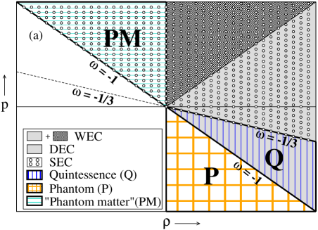
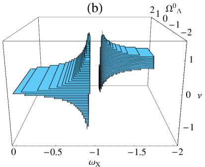
Figure 1: (a) The Weak (WEC, $\rho\geq 0$ and $\rho+p\geq 0$), Dominant (DEC, $\rho\geq|p|$ ) and Strong (SEC, $\rho+p\geq 0$ and $\rho+3p\geq 0$) energy conditions. The “standard” QE and phantom regions as well as the “Phantom Matter” ($\omega_{e}<-1$ with $\rho<0$) one are also shown; (b) The $3D$ volume formed by the points of the $\Lambda$XCDM parameter space that satisfy: i) the nucleosynthesis bound (12), ii) there is a turning point in the Universe evolution and iii) the relation $r(z)=\rho_{D}/\rho_{m}<10r_{0}$ holds for the whole Universe lifetime .

The points satisfying all three conditions constitute a significant part of the full parameter space as seen in the $3D$ plot in Fig.1(b). As an example, we consider the specific situation $\ -1-\delta<\omega_{X}<0$ and $\nu<1$. Looking at the system (3), we see that $\lambda_{1}>0\,,\lambda_{2}<0$, so there is a saddle point in the phase space, $\bar{\Omega}^{*}=\left(0,\Omega_{\Lambda}^{0},\Omega_{\Lambda}^{0}\right)^{t}$, from which trajectories diverge with the evolution (as $\zeta\rightarrow\infty$). This runaway, however, can be stopped provided $C_{1}<0$ in (9). Indeed, since the eigenvector ${\bf v_{1}}$ defines a runaway direction, if $C_{1}<0$ the third component of (8) will eventually become negative, and there will be a stopping. Using (12), the stopping condition acquires the form:

$$C_{1}=1-C_{2}-C_{3}=\frac{1-\Omega_{\Lambda}^{0}}{1-\nu}-\frac{\Omega_{M}^{0}(\omega_{m}-\omega_{X})}{\omega_{m}-\omega_{X}+\epsilon}\simeq\frac{1-\Omega_{\Lambda}^{0}}{1-\nu}-\Omega_{M}^{0}<0\,.$$ (17)

These features can be seen in Fig.2(a), where the trajectories corresponding to a fixed value of $\omega_{X}$ and $\nu$ and various values of $\Omega_{\Lambda}$ have been plotted in the ($\Omega_{m},\Omega_{D}$) plane. Only the curves that fulfil (17) get stopped. The Hubble function of one of the stopped trajectories is plotted in Fig.2(b), showing indeed the existence of a turning point, that in this case, as discussed in Sect.2, is due to the behavior of the cosmon as PM.

    

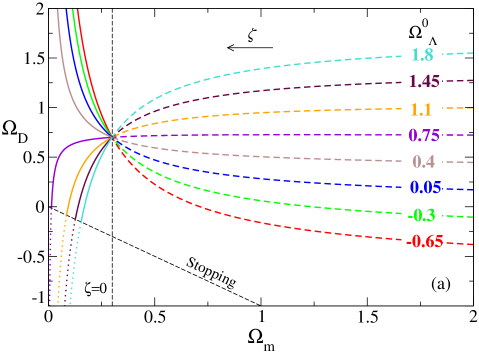
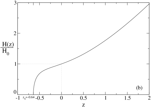
Figure 2: (a) Phase trajectories of the autonomous system (3) in the $(\Omega_{m},\Omega_{D})$ plane corresponding to $\omega_{X}=-1.85$, $\nu=-\nu_{0}$ ($\nu_{0}\equiv 0.026$) and differents choices of $\Omega_{\Lambda}^{0}$. Dashed lines show the parts of the curves corresponding to our past, full lines the parts between the present moment and the stopping (if there is stopping) and dotted lines the inaccessible part of the trajectory after the stopping; (b) the Hubble function $H=H(z)$ for the curve with: $\Omega_{\Lambda}^{0}=0.75$, showing the existence of a turning point.

The analysis of the EOS is one of the most important issues addressed in the present and future experiments. Recent combined data WMAP3Y suggest a value: $\omega_{\rm exp}=-1.06^{+0.13}_{-0.08}\,.$ This result does depend on the assumption that the EOS parameter does not evolve with time or redshift, so it is not directly applicable to the effective EOS of our model. Even so, we can find many scenarios that are in good agreement with it, as shown in Fig.3(a). We see that the value of $\nu$ modulates the behavior of the EOS, that can be QE-like (even though the $X$ is phantom-like!, see (2)), mimic that of a CC or present a mild evolution from the phantom to the QE region.

All the curves in Fig.3(a) satisfy (17), presenting a stopping point and therefore (c.f. Sect.3.1) a maximum of $r(z)$. This ratio is plotted in Fig.3(b) in units of its current value ($r_{0}\approx 7/3$), showing that $r(z)$ remains bounded and $\sim r_{0}$ for essentialy the entire Universe lifetime, which provides a natural solution to the coincidence problem. Let us stress that these features can occur even for $\nu=0$ (that is, for a strictly constant $\Lambda$).

    

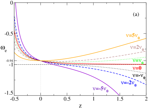
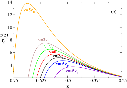
Figure 3: (a) Comparison of the effective EOS parameter of the $\Lambda$XCDM model, $\omega_{e}$, for $\omega_{X}=-1.85$, $\Omega_{\Lambda}^{0}=0.75$ and different values of $\nu$; (b) Same comparison for the maximum of the ratio $r=\rho_{D}/\rho_{m}$

5 Conclusions

We have shown that the $\Lambda$XCDM model can be in good agreement with present data and provide a solution to the cosmological coincidence problem as well as a clear signature. In our opinion the next generation of high precision cosmology experiments (DES, SNAP, PLANCK) SNAP should consider the possibility of a composite DE with dynamics controlled by the running of the cosmological parameters.

References

- (1) R. A. Knop et al., Astrophys. J. 598 (102) 2003; A.G. Riess et al. Astrophys. J. 607 (2004) 665.
- (2) D.N. Spergel et al., WMAP three year results: implications for cosmology, astro-ph/0603449.
- (3) M. Tegmark et al, Phys. Rev. D69 (2004) 103501.
- (4) P.J.E. Peebles, Astrophys. J. 284 (1984) 439.
- (5) S. Weinberg, Rev. Mod. Phys. 61 (1989) 1.
- (6) See e.g. E.J. Copeland, M. Sami, S. Tsujikawa, hep-th/0603057, and references therein.
- (7) U. Alam, V. Sahni, A.A. Starobinsky, JCAP 0406 (2004) 008.
- (8) H.K. Jassal, J.S. Bagla, T. Padmanabhan, Phys. Rev. D72 (2005) 103503.
- (9) J. Solà, H. Štefančić, Mod. Phys. Lett. A21 (2006) 479; Phys. Lett. 624B (2005) 147; J. Phys. A 39 (2006) 6753; J. Solà, J.Phys.Conf.Ser. 39 (2006) 179.
- (10) J. Grande, J. Solà, H. Štefančić, JCAP 0608 (2006) 011.
- (11) I. Shapiro, J. Solà, JHEP 0202 2002 006; Phys. Lett. 475B 2000 236.
- (12) R.D. Peccei, J. Solà, C. Wetterich, Phys. Lett. 195B (1987) 183.
- (13) J. Grande, J. Solà, H. Štefančić, Composite dark energy: cosmon models with running cosmological term and gravitational coupling, gr-qc/0609083.
- (14) I.L. Shapiro, J. Solà, C. España-Bonet, P. Ruiz-Lapuente, Phys. Lett. 574B (2003) 149; JCAP 0402 (2004) 006; I.L. Shapiro, J. Solà, Nucl. Phys. Proc. Supp. 127 (2004) 71; astro-ph/0401015.
- (15) P. G. Ferreira, M. Joyce, Phys. Rev. D58 (1998) 023503.
- (16) http://www.darkenergysurvey.org/; http://snap.lbl.gov/; http://www.rssd.esa.int/index.php?project=Planck.