Rotationally Modulated X-ray Emission from T Tauri Stars

Abstract

We have modelled the rotational modulation of X-ray emission from T Tauri stars assuming that they have isothermal, magnetically confined coronae. By extrapolating surface magnetograms we find that T Tauri coronae are compact and clumpy, such that rotational modulation arises from X-ray emitting regions being eclipsed as the star rotates. Emitting regions are close to the stellar surface and inhomogeneously distributed about the star. However some regions of the stellar surface, which contain wind bearing open field lines, are dark in X-rays. From simulated X-ray light curves, obtained using stellar parameters from the Chandra Orion Ultradeep Project, we calculate X-ray periods and make comparisons with optically determined rotation periods. We find that X-ray periods are typically equal to, or are half of, the optical periods. Further, we find that X-ray periods are dependent upon the stellar inclination, but that the ratio of X-ray to optical period is independent of stellar mass and radius.

1 Introduction

One of the recent results from the Chandra Orion Ultradeep Project (COUP) was the detection of significant rotational modulation of X-ray emission from low mass pre-main sequence stars. The detection of such modulation suggests that the coronae of T Tauri stars are compact and clumpy, with emitting regions that are inhomogeneously distributed across the stellar surface, and confined within magnetic structures that do not extend out to much beyond a stellar radius (Flaccomio et al., 2005). There is also evidence for much larger magnetic loops, possibly due to the interaction with a surrounding circumstellar disc (Favata et al., 2005; Giardino et al., 2006). A model already exists for T Tauri coronae, where complex magnetic field structures contain X-ray emitting plasma close to the stellar surface, whilst larger magnetic loops and open field lines are able to carry accretion flows (Jardine et al. 2006; Gregory et al. 2006).

In this paper we use surface magnetograms derived from Zeeman-Doppler imaging to extrapolate the coronae of T Tauri stars using stellar parameters taken from the COUP dataset (Getman et al., 2005). By considering isothermal coronae in hydrostatic equilibrium we obtain simulated X-ray light curves, for a range of stellar inclinations, and then X-ray periods using the Lomb Normalised Periodogram (LNP) method. We compare our results with those of Flaccomio et al. (2005), who demonstrate that those COUP stars which show clear evidence for rotationally modulated X-ray emission appear to have X-ray periods which are either equal to the optically determined rotation period ($P_{X}=P_{opt}$) or are half of it ($P_{X}=0.5P_{opt}$).

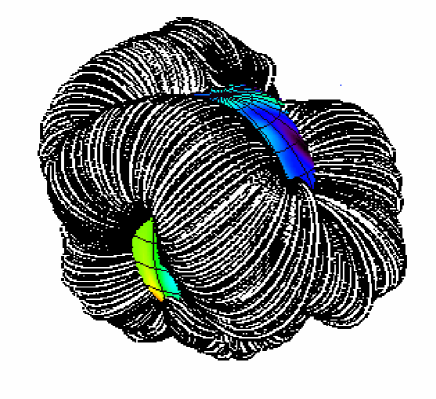
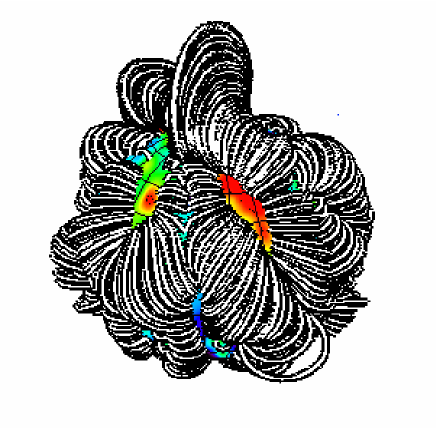
Figure 1: Closed coronal structures showing field lines which contain X-ray emitting plasma, extrapolated from surface magnetograms of (a) LQ Hya and (b) AB Dor, for COUP source number 6 ($M_{\ast}=0.23M_{\odot},R_{\ast}=1.6R_{\odot},P_{rot}=9.81d$). The magnetic structures are compact and inhomogeneously distributed about the stellar surface.

2 Realistic magnetic fields

In order to model the coronae of T Tauri stars we need to assume something about the form of the magnetic field. Observations suggest it is compact and inhomogeneous and may vary not only with time on each star, but also from one star to the next. To capture this behaviour, we use as examples the field structures of two different main sequence stars, LQ Hya and AB Dor determined using Zeeman-Doppler imaging (Donati & Collier Cameron 1997; Donati et al. 1997; Donati 1999; Donati et al. 1999; Donati et al. 2003). By using both stars, we can assess the degree to which variations in the detailed structure of a star’s corona may affect its X-ray emission. The method for extrapolating the field follows that employed by Jardine et al. (2002a) and is further detailed by Jardine et al. (2006) and Gregory et al. (2006); thus we provide only an outline here. Assuming the magnetic field $\mn@boldsymbol{B}$ is potential then $\nabla\times\mn@boldsymbol{B}=0$. This condition is satisfied by writing the field in terms of a scalar flux function $\Psi$, such that $\mn@boldsymbol{B}=-\nabla\Psi$. Thus in order to ensure that the field is divergence-free ($\nabla.\mn@boldsymbol{B}=0$), $\Psi$ must satisfy Laplace’s equation, $\nabla^{2}\Psi=0$; the solution of which is a linear combination of spherical harmonics,

$$\Psi=\sum_{l=1}^{N}\sum_{m=-l}^{l}\left[a_{lm}r^{l}+b_{lm}r^{-(l+1)}\right]P_{lm}(\theta){\rm e}^{{\rm i}m\phi},$$ (1)

where $P_{lm}$ denote the associated Legendre functions. The coefficients $a_{lm}$ and $b_{lm}$ are determined from the radial field at the stellar surface obtained from Zeeman-Doppler maps and also by assuming that at some height $R_{s}$ above the surface (known as the source surface) the field becomes radial and hence $B_{\theta}(R_{s})=0$, emulating the effect of the corona blowing open field lines to form a stellar wind (Altschuler & Newkirk, 1969). In order to extrapolate the field we used a modified version of a code originally developed by van Ballegooijen, Cartledge & Priest (1998).

For a given surface magnetogram we calculate the extent of the closed corona for a particular set of stellar parameters. This is achieved by calculating the hydrostatic pressure at each point along a field line loop. For an isothermal corona and assuming that the plasma along the field is in hydrostatic equilibrium then,

$$p=p_{0}\exp{\left(\frac{1}{c_{s}^{2}}\oint_{s}g_{s}ds\right)},$$ (2)

where $c_{s}$ is the isothermal sound speed and $g_{s}$ the component of the effective gravity along the field line such that, $g_{s}=\mn@boldsymbol{g}.\mn@boldsymbol{B}/|\mn@boldsymbol{B}|$. The constant $p_{0}$ is the gas pressure at a field line foot point and $p$ the pressure at some point along the field line. The effective gravity in spherical coordinates for a star with rotation rate $\omega$ is,

$$\mn@boldsymbol{g}\left(r,\theta,\phi\right)=\left(-\frac{GM_{\ast}}{r^{2}}+\omega^{2}r\sin^{2}{\theta},\omega^{2}r\sin{\theta}\cos{\theta},0\right).$$ (3)

We can then calculate how the plasma $\beta$, the ratio of gas to magnetic pressure, changes along each field line. If at any point along a field line $\beta>1$ then we assume that the field line is blown open. This effect is incorporated into our model by setting the coronal (gas) pressure to zero whenever it exceeds the magnetic pressure ($\beta>1$). We also set the coronal pressure to zero for open field lines. The gas pressure, and therefore the plasma $\beta$, is dependent upon the choice of $p_{0}$ which is a free parameter of our model. If we assume that the base pressure is proportional to the magnetic pressure then $p_{0}=KB_{0}^{2}$, a technique which has been used successfully to calculate mean coronal densities and X-ray emission measures for the Sun and other main sequence stars (Jardine et al. 2002a, b) as well as T Tauri stars (Jardine et al., 2006). By varying the constant $K$ we can raise or lower the overall gas pressure along field line loops. If the value of $K$ is large, many field lines would be blown open and the corona would be compact, whilst if the value of $K$ is small, then the magnetic field is able to contain more of the coronal gas. The extent of the corona therefore depends both on the value of $K$ and also on $B_{0}$ which is determined directly from surface magnetograms. For an observed surface magnetogram the base magnetic pressure $B_{0}$ varies across the stellar surface, and as such so does the base pressure $p_{0}$ at field line foot points. By considering stars from the COUP dataset Jardine et al. (2006) obtain the value of $K$ which results in the best fit to observed X-ray emission measures, for a given surface magnetogram. We have adopted the same values in this paper. We note that we make a conservative estimate of the location of the source surface by calculating the largest radial distance at which a dipole field line would remain closed, with the same average field strength. Fig. 1 shows examples of the complex magnetic field geometries which we consider.

The coronal field geometries which we consider in this work have been extrapolated from surface magnetograms of the young main sequence stars AB Dor and LQ Hya. In future it will be possible to use real T Tauri magnetograms dervied from Zeeman-Doppler images obtained using the ESPaDOnS instrument at the Canada-France-Hawaii telescope. However, in the meantime, the example field geometries shown in Fig. 1 capture three essential features of T Tauri coronae. First, Jardine et al. (2006) have already demonstrated that the field structures which we consider here yield X-ray emission measures and mean coronal densities which are consistent with values obtained during the COUP - the largest available dataset of X-ray properties of young stellar objects (Getman et al., 2005). Second, the fact that rotational modulation of X-ray emission was at all detected during the COUP automatically led to the conclusion that the dominant X-ray emitting regions must be compact and unevenly distributed across the star (Flaccomio et al., 2005). It can be seen from Fig. 1 that the X-ray emitting closed coronal field lines do not extent out to much beyond the stellar surface (the coronae are compact) and that the emitting regions are inhomogeneously distributed about the star (the coronae are clumpy), in immediate agreement with the COUP results. Further, as we discuss below, the field geometries considered in this paper do give rise to significant rotational modulation of X-ray emission. It can also be seen from Fig. 1 that some regions of the stellar surface do not contain regions of closed field, and would therefore be dark in X-rays. Such regions contain wind bearing open field lines. Third, observations of various classical T Tauri stars by Valenti & Johns-Krull (2004) show the line-of-sight (longitudinal) magnetic field components measured using photospheric absorption lines, are often consistent with a net circular polarisation signal of zero. However, strong fields are detected from Zeeman broadening measurements. Such polarisation measurements trace the surface field structure of T Tauri stars and immediately imply that such stars have complex and highly structured coronae. If the surface of the star is covered in many regions of opposite polarity this would give rise to a net polarisation signature of zero, with contributions to the overall signature from regions of opposite polarity cancelling out. Therefore the surface field must be highly complex and multipolar in nature, with many closed loops confining X-ray emitting plasma close to the surface of the star. However, it is also worth asking whether the coronal structure of classical T Tauri stars are likely to be fundamentally different from those of weak line T Tauri stars, a point which we discuss in §4.

Although we cannot be certain whether or not the magnetic field structures extrapolated from surface magnetograms of young main sequence stars in Fig. 1 do represent the magnetically confined coronae of T Tauri stars, they do satisfy the currently available observational constraints. They reproduce X-ray emission measures and coronal densities which are typical of T Tauri stars, and the field structures are complex, confining plasma within unevenly distributed magnetic structures close to the stellar surface. However, as such structures only represent a snap-shot in time of the coronal field geometry, we have chosen to consider two different field topologies. This allows us to model how much of an effect the field geometry has on the amplitude of modulation of X-ray emission and on resulting X-ray periods.

3 X-ray periods

3.1 X-ray light curves

Figure 2: The variation in X-ray emission measure (EM) with rotation phase for (a) the LQ Hya-like and (b) the AB Dor-like coronal structures as shown in Fig. 1, for inclinations of 30°(dashed), 60°(dotted) and 90°(solid). There is clear rotational modulation of X-ray emission.

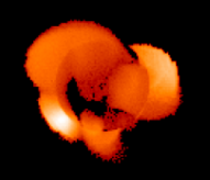
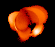
Figure 3: X-ray images obtained using the LQ Hya-like coronal structure from Fig. 1 for an inclination 90°(shown as the solid line in Fig. 2). Emitting regions are inhomogeneously distributed across the stellar surface and are confined within magnetic structures close to the star; some regions are, however, dark in X-rays. This particular surface map has two dominant emitting regions in opposite hemispheres, which at this inclination, go into eclipse as the star rotates giving rise to the two minima in Fig. 2 (solid line). Image (a) is for a rotational phase of 0.1, where the brightest of the two dominant emitting regions is in eclipse, (b) 0.4, where both of the dominant regions are visible, (c) 0.65, where the brightest emitting region is visible and the other is in eclipse and (d) 0.85, where once again both of the dominant regions can be seen.

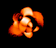
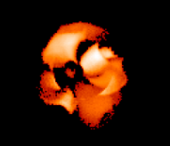
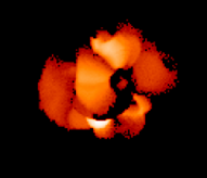
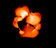
Figure 4: As Fig. 3 but using the AB Dor-like coronal structure from Fig. 1 and for an inclination of 30°(shown as the dashed line in Fig. 2). Image (a) is for a rotational phase of 0.15, (b) 0.35, (c) 0.6, where the amount of X-ray emission is at a maximum due to the brightest emitting region (towards the bottom of the image) being visible and (d) 0.85. The coronal structure is more clumpy than the LQ Hya-like field, with many bright emitting regions across the stellar surface.

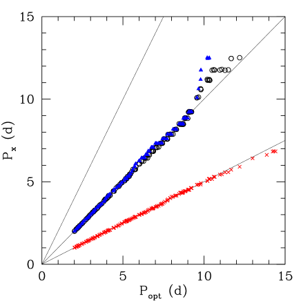
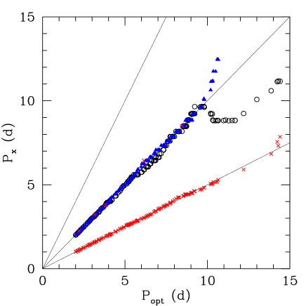
Figure 5: Comparison between X-ray periods $P_{X}$ and optically determined periods $P_{opt}$ for stars in the COUP dataset using (a) the LQ Hya-like (b) the AB Dor-like coronal structures shown in Fig. 1, for inclinations of $30\degr$(black circles), $60\degr$(blue triangles) and $90\degr$(red crosses). The solid lines represent $P_{X}=[0.5,1,2]P_{opt}$. The ratio $P_{X}/P_{opt}$ is independent of stellar mass and radius.

Once we have determined the structure of the closed corona we calculate the X-ray emission measure (EM) as described in Appendix A, and plot the ratio of EM to the maximum EM against rotational phase. Fig. 2 shows such plots using both the LQ Hya and AB Dor surface maps, for three inclinations. The corresponding X-ray images are shown in Figs. 3 and 4, from which it can be seen that emitting regions are compact and unevenly distributed across the stellar surface. However, some regions (which would contain open field lines) are dark in X-rays, in agreement with the conclusions of Flaccomio et al. (2005), that the saturation of activity cannot be due to the filling of the stellar surface with active regions.

For the LQ Hya-like coronal structure, although there are emitting regions across the stellar surface, there are two dominant emitting regions in opposite hemispheres, one of which is brighter in X-rays than the other. The effect of this is most apparent for large inclinations. For an inclination of $i=30\degr$ we see one minimum in the X-ray “light curve” (see Fig. 2), however as $i$ is increased to $60\degr$ we see the emergence of a second minimum, almost completely out of phase with the first. For $i=90\degr$ both of the dominant emitting regions go into eclipse as the star rotates, giving rise to the two distinct minima. As one of these dominant emitting regions is brighter in X-rays, however, the X-ray EM is further reduced when the brightest region goes into eclipse. The amplitude of the modulation is around 50%. For an inclination of $0\degr$ there is no rotational modulation of X-ray emission, as expected.

The AB Dor-like coronal structure is more complex and, in contrast to the LQ Hya-like coronal structure, there are many bright emitting regions (see Fig. 4). Fig. 2 shows the resulting X-ray light curves, and in this case we see little rotational modulation of the X-ray emission for $i=90\degr$, but see modulation of around 50% for smaller inclinations. It is already clear from the shapes of the X-ray light curves that the X-ray period depends on the stellar inclination.

3.2 X-ray and optical periods

We consider the same 233 COUP sources used in the analysis of Flaccomio et al. (2005), however, as our model requires estimates of the stellar parameters (mass, radius, rotation period and measurements from which we can infer a coronal temperature) we have omitted those sources without estimates of these parameters. This leaves a total of 183 COUP sources with a lower coronal temperature and 141 where a higher temperature component is also given in the COUP dataset. For each COUP source we have generated an X-ray light curve (see Fig. 6 for three examples) using both the LQ Hya and AB Dor surface magnetograms, and for inclinations of $30\degr$, $60\degr$ and $90\degr$. In the subsequent discussion we only consider the lower coronal temperature. Our results for the higher coronal temperature are similar and are discussed in §4. Each simulated light curve covers 13.2 days, to match the COUP observation time. COUP light curves also contain 5 gaps where the Chandra satellite passed through the Van Allen belts. Therefore we have considered both continuous light curves (see Fig. 6), and light curves which have gaps at approximately the same observation times (and lasting for approximately the same duration) as the gaps in COUP X-ray light curves (see Fig. 6). We tried sampling our simulated X-ray light curves every 2000s, 5000s and 10,000s, to match the analysis of Flaccomio et al. (2005), but found that our results were similar in all three cases. The results presented here refer only to a time sampling of 10,000s.

Figure 6: Light curves and Lomb Normalised Periodograms corresponding to inclinations of 30°(dashed), 60°(dotted) and 90°(solid), for the coronal structure in Fig. 1. The left hand column are the simulated light curves without gaps. However, when gaps are introduced into the light curves (right hand column) we find that the most significant peak in the LNP power spectrum generates the same X-ray period, albeit with lower significance. There are two significant peaks for the $i=90\degr$ case, one corresponding to $P_{opt}$ and the other $0.5P_{opt}$. The solid vertical line is the frequency corresponding to the optical period.

We have calculated X-ray periods using the Lomb Normalised Periodogram (LNP) method so that our analysis matches that of Flaccomio et al. (2005) as closely as possible. The observed X-ray light curves of COUP sources are contaminated with many flares, with a great variety of flaring behaviour, whereas our simulated light curves do not suffer from this problem. Therefore, when calculating X-ray periods, our false alarms probabilities (FAPs) indicating the significance of peaks found in the LNP power spectrum are vanishingly small, with $-40<log_{10}[FAP(\%)]<-10$.

Fig. 5 is a plot of our calculated X-ray periods against optically determined rotation periods from Flaccomio et al. (2005), which is collection of rotation periods taken mainly from Herbst et al. (2002). We have limited our search to X-ray periods of $P_{X}<13d$ and have chosen the scale of the axes to allow a direct comparison with similar plots in Flaccomio et al. (2005). For the LQ Hya-like coronal structure, at any given inclination, the ratio $P_{X}/P_{opt}$ is independent of stellar mass and radius, except for stars with large $P_{opt}$ (see the discussion below). We find that $P_{X}=P_{opt}$ for inclinations of $30\degr$ and $60\degr$, but that $P_{X}=0.5P_{opt}$ for $i=90\degr$. Flaccomio et al. (2005) provide a qualitative argument that the X-ray period would equal the optical period if there was one dominant emitting region on the stellar surface. They also point out that if there were two dominant emitting regions in opposite hemispheres, separated by $180\degr$ in longitude, then it should be expected that the X-ray period would be half of the optical period. Although we agree with this point of view, our LQ Hya-like field structure does have two dominant emitting regions in opposite hemispheres, which for high inclinations yields $P_{X}=0.5P_{opt}$ but at low inclinations gives $P_{X}=P_{opt}$. Therefore the qualitative picture of having two dominant emitting regions in opposite hemispheres giving rise to $P_{X}=0.5P_{opt}$ should come with the (perhaps obvious) caveat that it depends on the inclination at which the star is viewed.

Results for the AB Dor-like coronal structure are similar (see Fig. 5). We again find that the ratio $P_{X}/P_{opt}$ is independent of stellar mass and radius for the $i=30\degr$ and $60\degr$ cases, provided that $P_{opt}<10d$. Stars with $P_{opt}>10d$, and in particular those which have optical periods longer than the COUP observing time (13.2d), often do not have X-ray periods of either $0.5P_{opt}$ or $P_{opt}$. This is most noticeable for the AB Dor-like coronal structure in the $30\degr$ case (see Fig. 5), where stars with the longest $P_{opt}$ are found to have X-ray periods of $0.7P_{opt}$. This is a result of only considering the X-ray light curves over a duration equal to the COUP observing time. By extending our simulated X-ray light curves to cover twice the duration of the COUP observing time (so that $\approx 2$ complete rotations of stars with the longest $P_{opt}$ are covered by the light curves), we found that all X-ray periods in the $i=30\degr$ case clustered around $P_{X}=P_{opt}$. For the $i=90\degr$ case we find that most stars have $P_{X}=0.5P_{opt}$, but five stars have $P_{X}=P_{opt}$. This is due to there being two significant peaks in the LNP power spectrum (see Fig. 6) and, depending on which peak is the larger, the X-ray period is either 0.5$P_{opt}$ or $P_{opt}$. However, when the AB Dor-like coronal structure is viewed at an inclination of $90\degr$, the amount of rotational modulation of X-ray emission is at its smallest (only 13%) of all the field structures and inclinations which we have considered; this can be seen from the light curve in Fig. 2. Therefore the $i=90\degr$ case for the AB Dor-like field is an interesting result. It shows that it is possible to have a highly structured corona, with emitting regions which are close to the stellar surface, with regions which are dark in X-rays, but when such a field structure is viewed at an unfavourable inclination, little rotational modulation of X-ray emission is detected, and it is difficult to recover an X-ray period. However, there is significant modulation detected for the $i=30\degr$ and $60\degr$ cases with $P_{X}=P_{opt}$. Therefore the X-ray periods we have determined are similar for both the AB Dor and LQ Hya-like coronal fields, and are dependent on the stellar inclination. The AB Dor field has many bright emitting regions making it difficult to qualitatively understand the exact shape of the resulting X-ray light curve. In the next section we further investigate the effects of inclination and the magnetic field structure on X-ray periods.

We have also considered how having gaps in our simulated X-ray light curves would affect the resulting X-ray period (see Fig. 6). We found that the values of $P_{X}$ obtained from light curves with gaps were identical to those derived from continuous light curves, with the only difference being that the main peaks in the LNP power spectra were of lower significance.

3.3 Effect of inclination and coronal structure

In order to further investigate the effects of inclination and the structure of stellar coronae, we randomly assign an inclination of between $5\degr$ and $90\degr$ to each of the COUP sources before calculating an X-ray period. Inclinations of smaller than $\approx 5\degr$ produce little or no rotational modulation of X-ray emission and so are not considered. The results are plotted in Fig. 7 for both the LQ Hya and AB Dor-like coronal structures. We again find that X-ray periods are either equal to $P_{opt}$ or $0.5P_{opt}$, with a few exceptions.

Our simulations apparently highlight a well defined lower limit for X-ray periods of $P_{X}=0.5P_{opt}$. It should be noted, however, that we are limited by the number of surface maps which we have available; it could be the case that another surface magnetogram may yield X-rays periods which are lower that $0.5P_{opt}$. Flaccomio et al. (2005) find stars with reliably detected rotational modulation of X-ray emission with $P_{X}<0.5P_{opt}$ but argue that such period detections may be spurious. In order to test if there is a well defined lower limit of $P_{X}=0.5P_{opt}$ we generated a model coronal structure which had three emitting regions randomly positioned around the stellar surface. In the case where all three emitting regions were evenly spaced in longitude, and a fixed (low) latitude (e.g. the three emitting regions placed at equal increments about the star’s equator) we found X-ray periods of $P_{X}=0.333P_{opt}$. Therefore it is possible to have a coronal field where the dominant emitting regions are distributed such that $P_{X}<0.5P_{opt}$. However, we find that such field structures are rare in comparison to those which yield $P_{X}=[0.5,1]P_{opt}$.

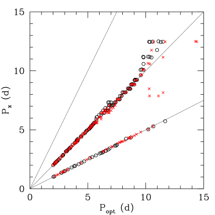
Figure 7: Comparison between our calculated X-ray periods and observed optical periods. X-ray periods have been calculated for COUP stars from Flaccomio et al. (2005) with randomly assigned inclinations. The lines represent $P_{X}=[0.5,1,2]P_{opt}$, with data for the LQ Hya-like (black circles) and AB Dor-like coronal structures (red crosses). There is little difference between the different coronal field geometries.

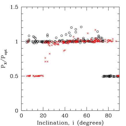
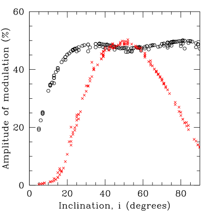
Figure 8: (a) The variation in X-ray period as a fraction of the optical period with stellar inclination for the LQ Hya (black circles) and AB Dor (red crosses) coronal fields. Data represents the same stars as in Fig. 7 with the same randomly selected inclinations, with (b) the amplitude of modulation of X-ray emission.

Flaccomio et al. (2005) also find a few stars with evidence for rotationally modulated X-ray emission with X-ray periods which are larger than the optical period, however their further simulations appear to indicate that these period detections (in particular those with $P_{X}>2P_{opt}$) are likely to be spurious. We could not create any model which led to a $P_{X}$ value of much larger than $P_{opt}$.

The X-ray period depends on stellar inclination (see Fig. 8). At low inclinations for the LQ Hya field, $P_{X}=P_{opt}$. As the inclination is increased a second peak in the LNP power spectrum becomes stronger and eventually, for $i\approx 75\degr$, both peaks are of almost equal significance. For $i>75\degr$, $P_{X}=0.5P_{opt}$, with the secondary peak having become the most significant. This occurs when both of the dominant emitting regions enter eclipse at different times as the star rotates. At low inclinations the amplitude of modulation is small (see Fig. 8) for the LQ Hya field, but is almost constant for $i>25\degr$. Overall we find less modulation for the AB Dor field. This is consistent with our finding from §3.2. When the AB Dor field is viewed at both low ($i<30\degr$) and high ($i>75\degr$) inclinations there is little rotational modulation of X-ray emission. Thus, simply having compact emitting regions inhomogeneously distributed about the stellar surface is not enough to generate large modulation of X-ray emission - the amount of modulation depends strongly on the stellar inclination.

4 Summary and Discussion

By extrapolating surface magnetograms of young main sequence stars we have shown that magnetic fields with a realistic degree of complexity reproduce the observed rotational modulation of X-ray emission from T Tauri stars (Flaccomio et al., 2005). This model has already been used to correctly predict X-ray EMs, mean coronal densities and the observed increase in X-ray EM with stellar mass (Jardine et al., 2006). We find that X-ray emitting regions are inhomogeneously distributed around the stellar surface and are typically compact ($\la R_{\ast}$). This agrees with the findings of Flaccomio et al. (2005) who point out that in order to explain the amplitude of the modulation of X-ray emission which they detect, emitting regions must be compact in order to undergo eclipse.

We found that the ratio $P_{X}/P_{opt}$ is independent of stellar mass and radius, but that X-ray periods are dependent on stellar inclination. For example, in the case where there are two dominant X-ray emitting regions in opposite hemispheres, we found that the X-ray period could be either $0.5P_{opt}$ or $P_{opt}$ depending on how the star is inclined to the observer. In order words, the presence of two bright emitting regions in opposite hemispheres does not immediately imply that $P_{X}=0.5P_{opt}$. Further, some coronal fields with compact emitting regions produce only small amplitude modulation of X-ray emission when viewed at unfavourable inclinations.

We do not find X-ray periods of $P_{X}>2P_{opt}$, unlike Flaccomio et al. (2005). However, they argue that those period detections are likely to spurious, given the arduous task of removing flares from observed COUP X-ray light curves. Also the apparent lower limit of $P_{X}=0.5P_{opt}$ may not be of true physical origin. We have demonstrated this by constructing a corona which resulted in $P_{X}=0.333P_{opt}$; however this sort of field structure is perhaps uncommon. Instead the majority of X-ray periods cluster around $P_{X}=[0.5,1]P_{opt}$. We found that $P_{X}$ (for a fixed inclination) was the same for both the LQ Hya and AB Dor-like coronal fields, despite the distribution of emitting regions being different for the two cases. This suggests that for complex magnetic fields, where there are many emitting regions distributed across the stellar surface, it becomes difficult to disentangle the contribution to the X-ray emission from any particular emitting region. Consequently, even though different stars are likely to have different coronal structures, the X-ray periods of T Tauri stars appear to cluster around $P_{opt}$ and $0.5P_{opt}$. In other words, although different coronal structures give rise to different amounts of modulation at a fixed inclination, the X-ray period is likely to be the same.

Throughout we have only considered the lower coronal temperatures derived from the COUP dataset. If instead we had used the higher coronal temperatures our results and conclusions remain the same. For a higher coronal temperature more field lines are unable to contain the coronal gas and are blown open to form a stellar wind, meaning that coronae are (slightly) more compact. This leads to small, but not important, differences in the resulting X-ray periods, however the amplitude of modulation is larger (typically 60% compared with 50% for the lower coronal temperatures). The amplitudes of modulation which we determine compare well with the observed values of Flaccomio et al. (2005) of 20-70%.

Although we have not considered it in this paper, the coronal structure of T Tauri stars may evolve on timescales that are comparable with the COUP observing time. For example a dominant X-ray emitting region may be lost due to a large coronal mass ejection which would open up a previously-closed region of field. This may then change the resulting X-ray period. However, it is still interesting that even with two different field structures such as those in Fig. 1, the X-ray periods are still typically equal to the optical period or are half of the optical period.

We have not considered how the presence of a circumstellar disc and active accretion influences coronal structures, and the possible resulting effects on the X-ray period/amplitude of modulation. A comprehensive and detailed discussion of how accretion processes may influence X-ray emission in T Tauri stars is provided by Preibisch et al. (2005). The growing consensus, as was confirmed by COUP, is that X-ray emission from T Tauri stars does not depend upon the presence of a disc, but is influenced by active accretion. For example, Feigelson et al. (2002) found X-ray activity levels were the same for stars with and without discs. However, Flaccomio et al. (2003) found a difference in the X-ray activity levels of accreting and non-accreting stars. The process of accretion therefore influences the amount of X-ray emission detected, with stars that show evidence for accretion having X-ray luminosities which are a factor of 2-3 smaller than those stars without discs and those stars which show evidence for discs, but not for accretion (Preibisch et al., 2005).

Accretion may therefore affect the coronal structure of T Tauri stars, which in turn may have implications for rotational modulation of X-ray emission, and X-ray periods. It is important to note however that Flaccomio et al. (2005) have searched for correlations between observed modulation amplitudes and the $\Delta$(I$-$K) excess, a disc indicator, and EW(CaII), an accretion indicator, but do not find any. Furthermore, Flaccomio et al. (2005) also search for dependencies on the X-ray period detection fraction with the indicators of discs and accretion, but again find none. This suggests that there is no difference in the spatial distribution of X-ray emitting regions in both classical and weak line T Tauri stars (with the former having both a disc and active accretion, and the latter neither). However, Flaccomio et al. (2005) did find a suggestion (but with a low significance of only about $1\%$) that stars with $P_{X}=0.5P_{opt}$ are preferentially active accretors.

Jardine et al. (2006) have shown that stars (typically of lower mass) which have coronae that would naturally extend to beyond the corotation radius would have their outer corona stripped by the presence of a disc. In order to check if this would affect the resulting X-ray period we determined the coronal structure of all the stars considered in §3 assuming that they were surrounded by a disc. Any field line which passed through the disc at, or within the corotation radius was assumed to have the ability to carry an accretion flow and was therefore considered to be “mass-loaded” and set to be dark in X-rays - a process which is discussed in detail by Jardine et al. (2006) and Gregory et al. (2006). We then calculated X-ray emission measures with rotational phase and determined the amplitude of modulation of X-ray emission and X-ray periods, using the same methods as discussed in §3. We found no difference in the values of $P_{X}$ and very little difference in the amplitudes of modulation. We therefore conclude, exactly as the observations suggest, that the presence of discs does not influence rotational modulation of X-ray emission. However, active accretion might.

We have yet to consider how accretion could influence rotational modulation of X-ray emission. As already discussed above stars which are actively accreting show lower levels of X-ray activity than those which are non-accretors. Again, the possible explanations for this are discussed by Preibisch et al. (2005), with the most likely being that magnetic reconnection events in the magnetosphere cannot heat the dense material within accretion columns to a high enough temperature to emit in X-rays. Some models suggest that accretion will distort magnetic field lines giving rise to instabilities and reconnection events (e.g. Romanova et al. 2004). The energy liberated in such reconnection events may not be able to heat the high density material in accretion columns to a sufficiently high temperature in order to emit in X-rays. Thus accretion columns rotating across the line-of-sight to the star may be responsible for the observed reduction in X-ray emission in accreting T Tauri stars compared with the non-accretors. The effect of this on X-ray periods and modulation amplitudes will be considered in future work. A detailed accretion flow model will have to be constructed in order to account for the attenuation of coronal X-rays by accretion columns rotating across the line-of-sight. Also, inner disc warps may have a similar effect at high stellar inclinations. This could change the shape of the X-ray variability curves shown in Figs. 2 and 6, with a reduction in X-ray emission at particular rotational phases, depending on the accretion flow geometry.

Our model may allow for the simultaneous confinement of X-ray emitting plasma in closed loops close to the stellar surface, but also for other field lines to stretch out into the inner disc and carry accretion flows. Gregory et al. (2006) find that often open field lines can carry accretion flows, which may allow accretion to influence the magnetic field structure on the large scale, with field lines being “mass-loaded” with disc material, but leaving compact coronae relatively unaffected by the process of accretion. This model would allow for the existence of large extended magnetic structures, inferred to exist from the detection of large flaring loops by Favata et al. (2005), with the coexistence of compact coronae. However, much quantitative work remains to be done here. Another new accretion model may offer insights into the connection between X-ray emission and accretion in T Tauri stars. An MHD model by von Rekowski & Piskunov (2006) suggests that rather than material being loaded onto field lines at the inner edge of the disc, it flows onto the star only at times when, and into regions where, the accretion flow is able to overcome the stellar wind. In such a way this model predicts that accretion only occurs into regions of low field strength. It is also worth noting the observational results of Flaccomio et al. (2005) that indicate that rotational modulation of X-ray emission is not preferentially detected in either accreting or non-accreting T Tauri stars and that therefore the spatial structure of the X-ray emitting plasma is the same in both cases. Hence, although accretion does affect X-ray emission in accreting stars, and may distort the structure of stellar coronae, it may not affect the existence of rotational modulation.

Appendix A Determining X-ray Emission Measures

In deriving expressions for the variation of the emission measure with radial distance from the star, we begin with (2). If we scale all distances to a stellar radius, we can write

$$p(r,\theta)=p_{\ast}(1,\theta)\exp\left[\Phi_{g}\left(\frac{1}{r}-1\right)+\Phi_{c}\sin^{2}\theta(r^{2}-1)\right]$$ (4)

where $p_{\ast}(1,\theta)$ is the pressure distribution across the stellar surface and

$$\Phi_{g} = \frac{GM/R_{\ast}}{k_{B}T/m}$$ (5)

$$\Phi_{c} = \frac{\omega^{2}R_{\ast}^{2}/2}{k_{B}T/m}$$ (6)

are the surface ratios of gravitational and centrifugal energies to the thermal energy. The emission measure $EM=\int n_{e}^{2}dV$ is then

$$EM = \frac{4\pi R_{\ast}^{3}}{(k_{B}T)^{2}}$$

$$\int_{\theta_{m}}^{\pi/2}p_{\ast}^{2}(1,\theta)\exp\left[-2\Phi_{c}\cos^{2}\theta(r^{2}-1)\right]\sin\theta d\theta$$

$$\int_{1}^{r_{m}}r^{2}\exp\left[2\Phi_{g}\left(\frac{1}{r}-1\right)+2\Phi_{c}(r^{2}-1)\right]dr.$$

With the substitution $\mu=\cos\theta$ such that $\mu_{m}=\cos\theta_{m}=(1-r/r_{m})^{1/2}$, the $\theta$-integral can be written as

$$\int_{0}^{\mu_{m}}p_{\ast}^{2}(1,\theta)\exp\left[-2\Phi_{c}\mu^{2}(r^{2}-1)\right]d\mu$$ (8)

which, on using the substitution $t=[2\Phi_{c}(r^{2}-1)]^{1/2}\mu$, gives

$$\frac{1}{\left[2\Phi_{c}(r^{2}-1)\right]^{1/2}}\int_{0}^{t_{m}}p_{\ast}^{2}(1,\theta)e^{-t^{2}}dt$$ (9)

where $t_{m}=[2\Phi_{c}(r^{2}-1)]^{1/2}[1-r/r_{m}]^{1/2}$. Assuming that the pressure is uniform over the stellar surface we obtain the following expression for the emission measure as a function of $r$:

$$EM(r) = \sqrt{\frac{2\pi^{3}}{\Phi_{c}}}\frac{R_{\ast}^{3}p_{\ast}^{2}}{(k_{B}T)^{2}}$$

$$\int_{1}^{r_{m}}\frac{r^{2}}{(r^{2}-1)^{1/2}}{\rm erf}\left[2\Phi_{c}(r^{2}-1)\left(1-\frac{r}{r_{m}}\right)\right]^{1/2}$$

$$\exp\left[2\Phi_{g}\left(\frac{1}{r}-1\right)+2\Phi_{c}(r^{2}-1)\right]dr.$$

where we remind the reader that all distances $r$ have been scaled to a stellar radius.

References

- Altschuler & Newkirk (1969) Altschuler M. D., Newkirk G., 1969, SoPh, 9, 131
- Donati (1999) Donati J.-F., 1999, MNRAS, 302, 457
- Donati & Collier Cameron (1997) Donati J.-F., Collier Cameron A., 1997, MNRAS, 291, 1
- Donati et al. (1999) Donati J.-F., Collier Cameron A., Hussain G. A. J., Semel M., 1999, MNRAS, 302, 437
- Donati et al. (2003) Donati J.-F. et al. 2003, MNRAS, 345, 1145
- Donati et al. (1997) Donati J.-F., Semel M., Carter B. D., Rees D. E., Collier Cameron A., 1997, MNRAS, 291, 658
- Favata et al. (2005) Favata F., Flaccomio E., Reale F., Micela G., Sciortino S., Shang H., Stassun K. G., Feigelson E. D., 2005, ApJS, 160, 469
- Feigelson et al. (2002) Feigelson E. D., Broos P., Gaffney III J. A., Garmire G., Hillenbrand L. A., Pravdo S. H., Townsley L., Tsuboi Y., 2002, ApJ, 574, 258
- Flaccomio et al. (2003) Flaccomio E., Damiani F., Micela G., Sciortino S., Harnden Jr. F. R., Murray S. S., Wolk S. J., 2003, ApJ, 582, 398
- Flaccomio et al. (2005) Flaccomio E., Micela G., Sciortino S., Feigelson E. D., Herbst W., Favata F., Harnden F. R., Vrtilek S. D., 2005, ApJS, 160, 450
- Getman et al. (2005) Getman K. V. et al. 2005, ApJS, 160, 319
- Giardino et al. (2006) Giardino G., Favata F., Silva B., Micela G., Reale F., Sciortino S., 2006, A&A, 453, 241
- Gregory et al. (2006) Gregory S. G., Jardine M., Simpson I., Donati J.-F., 2006, MNRAS, 371, 999
- Herbst et al. (2002) Herbst W., Bailer-Jones C. A. L., Mundt R., Meisenheimer K., Wackermann R., 2002, A&A, 396, 513
- Jardine et al. (2006) Jardine M., Cameron A. C., Donati J.-F., Gregory S. G., Wood K., 2006, MNRAS, 367, 917
- Jardine et al. (2002a) Jardine M., Collier Cameron A., Donati J.-F., 2002a, MNRAS, 333, 339
- Jardine et al. (2002b) Jardine M., Wood K., Collier Cameron A., Donati J.-F., Mackay D. H., 2002b, MNRAS, 336, 1364
- Preibisch et al. (2005) Preibisch T. et al. 2005, ApJS, 160, 401
- Romanova et al. (2004) Romanova M. M., Ustyugova G. V., Koldoba A. V., Lovelace R. V. E., 2004, ApJL, 616, L151
- Valenti & Johns-Krull (2004) Valenti J. A., Johns-Krull C. M., 2004, Ap&SS, 292, 619
- van Ballegooijen et al. (1998) van Ballegooijen A. A., Cartledge N. P., Priest E. R., 1998, ApJ, 501, 866
- von Rekowski & Piskunov (2006) von Rekowski B., Piskunov N., 2006, Astron. Nachr., 327, 340