Constraints on the nature of dust particles by infrared observations

Abstract

The far-infrared (FIR) emissivity of dust is an important parameter characterizing the physical properties of the grains. With the availability of stellar databases and far-infrared data from Infrared Space Observatory (ISO) it is possible to compare the optical and infrared properties of dust, and derive the far-infrared emissivity with respect to the optical extinction. In this paper we present the results of a systematic analysis of the FIR emissivity of interstellar clouds observed with ISOPHOT (the photometer onboard ISO) at least at two infrared wavelengths, one close to $\sim$100$\mu$m and one at 200$\mu$m. We constructed FIR emission maps, determined dust temperatures, created extinction maps using 2MASS survey data, and calculated far-infrared emissivity for each of these clouds. We present the largest homogeneously reduced database constructed so far for this purpose. During the data analysis special care was taken on possible systematic errors. We find that far-infrared emissivity has a clear dependence on temperature. The emissivity is enhanced by a factor of usually less than 2 in the low dust temperature regime of 12K$\leq$T_d$\leq$14K. This result suggests larger grain sizes in those regions. However, the emissivity increase of typically below 2 restricts the possible grain growth processes to ice-mantle formation and coagulation of silicate grains, and excludes the coagulation of carbonaceous particles on the scales of the regions we investigated. In the temperature range 14 K $\leq$ T_d $\leq$ 16 K a systematic decrease of emissivity is observed with respect to the values of the diffuse interstellar matter. Possible scenarios for this behaviour are discussed in the paper.

1 Introduction

The far-infrared (FIR) emissivity of interstellar grains predominantly emitting at wavelengths in excess of 100 $\mu$m can now be determined in many molecular and moderate density regions thanks to the increasing availability of far-infrared, sub-mm, and massive stellar data sets. Several studies have reported on the detection of an enhancement of the FIR emissivity in the 100-200 $\mu$m wavelength range in regions of higher column density compared to the dust emissivity in the diffuse interstellar medium associated with HI (Bernard et al., 1999; Cambrésy et al., 2001; Juvela et al., 2002; Stepnik et al., 2003; Lehtinen et al., 2004, Rawlings et al., 2005). The largest sample of different regions is presented in del Burgo et al. (2003) presenting a study of eight translucent clouds.

The observations suggest a trend where the emissivity increases with decreasing temperature. The variation is attributed to a change in grain properties which is expected to take place in denser environments. In particular, the increase in emissivity is interpreted as a signature of an enhancement in grain size.

However, the trend shows a large scatter which might be due to the observational limitations which increase the uncertainties. On one hand, star counts statistically probe only a limited extinction range and, on the other hand, the determination of the grain temperatures in the infrared can have large uncertainties.

In this study we present a large sample based on Infrared Space Observatory (ISO) data of cloud regions with reliable values of the FIR dust emissivity and optical extinction data. We examine in detail the possible observational and data processing errors to ensure the reliability of our results. A general good agreement was found between our results and previous studies of individual regions. Due to the large number of data points we are able to put stronger constraints on the emissivity changes with temperature.

2 Observations and data reduction

2.1 Far-infrared maps

We searched the ISO Archive (Salama 2004) for ISOPHOT observations (Lemke et al. 1996) of interstellar clouds matching the following criteria: (1) the field has been covered at least at two far-infrared wavelengths: one at 200 $\mu$m (long) and another either at 90, 100 or 120 $\mu$m (short) in order to provide a sufficient wavelength interval for a reliable colour temperature calculation; (2) the cloud has to be galactic and must have sufficient dynamic range in brightness for correlation analyses; (3) the map is larger than 5′  at least in one dimension; and (4) there is no high mass star formation going on in the vicinity of the cloud which could significantly change the local interstellar radiation field. In total we selected 22 maps which is the largest sample evaluated so far for studying far-infrared dust emissivity. All selected maps were obtained with the P22 astronomical observing template mode (Laureijs et al. 2003). Measurement wavelengths, ISO-id numbers and central positions are listed in Table 1.

The ISOPHOT observations were performed with the C100 (43$\aas@@fstack{\prime\prime}$5$\times$43$\aas@@fstack{\prime\prime}$5 sized pixels) and C200 (89$\aas@@fstack{\prime\prime}$5$\times$89$\aas@@fstack{\prime\prime}$5 sized pixels) cameras. The ISOPHOT data were processed with the Phot Interactive Analysis software version 10.0 (PIA, Gabriel et al., 1997), using standard batch processing and a first quartile flatfielding. We followed in detail the processing scheme described in del Burgo et al. (2003). The data were colour corrected taking into account the dust temperature derived from the brightness ratio at the two wavelengths (see Sect. 3.1).

The officially quoted absolute photometric uncertainty of the surface brightness in the ISO Legacy Archive is $\leq$20–25% (Klaas et al., 2003). In the present study we estimated independently this uncertainty in two ways. We compared the ISOPHOT and COBE/DIRBE background surface brightness values, interpolated to the ISOPHOT wavelengths (1) for a large sample of mini-map observations and (2) for our target fields. This analysis is presented in Appendix A. The results of this investigation show, that the typical relative deviations of the individual ISOPHOT measurements with respect to the COBE/DIRBE values is $\sim$15%, and that there is no noticable systematic discrepancy between the two photometric systems. Throughout this paper we present our results in the ISOPHOT/PIA 10.0 surface brightness photometric system. The effect of a potential imperfect surface brightness calibration is discussed in detail in Sect. 4.5, based on results presented in Appendix A.

2.2 Extinction Data

The traditional method to derive extinction in interstellar clouds is based on variations in stellar density in the sky due to the obscuration of dust (Wolf 1923). Star counts obtained by placing a regular grid on the target field are converted to B or V-band extinction using statistical methods; the zero extinction level is obtained by comparison with a nearby extinction free reference field.

Cambrésy et al. (1997) replaced the classical regular grid with an adaptive one; in this method the gridsize is adjusted to include a fixed number of stars, therefore it can still provide extinction estimates for high density regions. However, in these cases the derived A_V values are averages over the enlarged area of the adaptive cell.

Due to the requirement of sufficient count of stars for reliable statistics, the minimum resolution is limited to arcminute scales, and low dust column densities. The maximum extinction in the visual is at best 5 mag and cannot be improved significantly by deep dedicated observations. In that respect, online catalogues with optical stellar data are well suited for the method.

In recent years the application of near-infrared reddening of individual stars has become widely used due to the general availability of J, H and K-band measurements. Extinction mapping methods using NIR reddening often combine the individual reddening values in some statistical manner in order to minimize the effect of individual line of sights. The NICE and NICER colour excess methods (Lada et al. 1994, Lombardi & Alves 2001) proved to produce good quality maps in many applications. Although NIR star counts are more reliable for high extinction values, in the low to intermediate extinction range (A_V $\leq$ 15 mag) the NIR colour excess methods are superior over NIR star counts, since they are less affected by the presence of foreground stars (Cambrésy et al. 2002).

The 2MASS Point Source Catalogue (Cutri et al. 2003) is a powerful source of NIR data and can be used to obtain NIR colour excess / extinction as was done by many authors in recent years.

A detailed comparison of visual extinctions obtained by optical star count and NIR colour excess is presented in Kiss et al. (2006). In this paper extinction maps are derived using star counts of USNO data (Monet et al., 1998, 2003) and using near-infrared (J, H and K_S-band) reddening of 2MASS data. Their fig. 2 shows a good correlation of the two datasets and the slope of the scatter plot is very near to unity for low extinctions. A flattening of the USNO extinction occurs at 3…3.5 mag, due to the already insufficient count statistics at these extinction levels.

The near-infrared colour excess methods are less affected by uncertainties due to foreground stars and give reliable extinction values in denser regions up to $\sim$15 mag. Therefore we decided to apply the NICER method on the 2MASS Point Source Catalogue to obtain extinction maps in this paper. Following the findings by Cambrésy et al. (2002) we set A${}_{\rm V}^{\rm lim}$ = 8 mag for the liming magnitude of 2MASS data, assuming a 10% of foreground stars in the target field. Above this limit we did not consider the extinction data to be reliable. These data points were excluded from the further analysis. Due to the low number of data points above this limit and outlier resistant routines we used in the scatter plot analysis, difference between the effect of a cut in A_V or of a cut perpendicular to the slope at A${}_{\rm V}^{\rm lim}$ = 8 mag is negligible.

3 Results

3.1 Dust temperature

Figure 1: Example (a) of a short versus long wavelength surface brightness scatter plot and (b) a visual extinction versus 200 $\mu$m scatter plot, both in the G100.0+14.8 field. On both panels the dashed lines show the fitted linears.

We derived colour temperatures T_d from the slope in the I${}_{\lambda_{1}}$ versus I${}_{\lambda_{2}}$ scatter plot of a specific sky region, where I${}_{\lambda_{1}}$ and I${}_{\lambda_{2}}$ are the surface brightness values at the wavelengths $\lambda_{1}$ and $\lambda_{2}$, respectively. An example in shown in Fig. 1a. Maps taken with the C100 camera (90 and 100 $\mu$m) were smoothed to the resolution of the 200 $\mu$m observation. The method of using scatter plots to determine T_d is described in del Burgo et al. (2003). It has the main advantage that the slope is insensitive to surface brightness offsets due to e.g. zodiacal light, extragalactic background, calibrational zero point, etc. The conversion of the $\Delta\rm I_{\lambda_{1}}/\Delta\rm I_{200}$ slopes to T_d was done via high resolution $\Delta\rm I_{\lambda_{1}}/\Delta\rm I_{200}$– T_d tables, assuming a $\nu^{\beta}\rm B_{\nu}\rm(T)$ spectral energy distribution. The tables also accounted for the correct colour correction. We adopted $\beta$ = 2.

In Sect. 4.3 we check the effect of a different emissivity law. In the following we adopt T_d as an approximation of the physical temperature of the dust grains.

Del Burgo et al. (2003) found that the scatter plots of some fields can consist of more than one linear section, indicating multiple dust temperatures within the field. Inspection of the maps of these fields indicated that the different temperature components came from interlocked regions which could be separated by A_V isocontours. The resulting I${}_{\lambda_{1}}$ versus I₂₀₀ scatter plots of the subfields were sufficiently linear.

The uncertainty in the temperature T_d can be attributed to, firstly, the error in the slope $\delta(\Delta\rm I_{\lambda_{1}}/\Delta\rm I_{200})$, and, secondly, the calibration uncertainty in the surface brightness values. The first component was computed from the formal uncertainty of the linear fits. The second component was evaluated by using surface brightness uncertainty values given in Sect. 2.1. The resulting temperature and uncertainty values are typically in the order of 0.7 K depending on the colour temperature (Table 1.)

3.2 Emissivity parameters

In Table 1 we list the derived values of I₂₀₀/A_V obtained from the slopes of the I₂₀₀ versus A_V relationships in those regions where T_d is constant as delineated by a constant I${}_{\lambda_{1}}$ vs. I₂₀₀. The 200$\mu$m surface brightness was smoothed to the resolution of A_V. The ratio I₂₀₀/A_V consists of two independent observables and therefore also serves as a good diagnostics of the main uncertainties. An example A_V vs. I₂₀₀ scatter plot is presented in Fig. 1b.

Using the measured value of T_d from the ratio $I_{\lambda_{1}}/I_{200}$, we derive the ratio between the infrared and optical opacity $\tau_{200}$/A_V from $\tau_{200}$/A_V  = (I₂₀₀/A_V) $\times$ B₂₀₀(T_d)^-1, where B₂₀₀(T_d) is the Planck function at 200 $\mu$m at the dust temperature T_d.

Altogether, we derived 26 sets of T_d, I₂₀₀/A_V and $\tau_{200}$/A_V values in the 22 maps, due to multiple temperature components in 4 fields. In addition, six fields of the del Burgo et al. (2003) sample have been reprocessed following our scheme (see Table 1).

The errors of $\tau_{200}$/A_V come from two sources: from the error in the determination of I₂₀₀/A_V in the I₂₀₀ versus $A_{\rm V}$ scatter plot and from the temperature uncertainty in B${}_{\nu}\rm(T)$. Assuming that these two sources are independent, the final $\tau_{200}$/A_V errors can be expressed via the partial derivatives by I₂₀₀/A_V and B${}_{\nu}\rm(T)$, following standard error propagation. Since we use the slope of the I₂₀₀ versus A_V relation only, systematic offsets in I₂₀₀ and A_V – like in the temperature computation – do not play a role.

To determine the propagation of the error in T_d in the Planck function, we use the two values T–$\delta$T and T+$\delta$T to estimate the upper and the lower error bars in $\tau_{200}$/A_V. In most cases the upper and lower error bars are nearly similar, therefore we give one average value for the uncertainty in Table 1. In the subsequent figures we present these upper and lower error bars individually. The relative errors caused by the temperature uncertainties are typically much larger than the relative errors from the determination of I₂₀₀/A_V in the scatter plots.

3.3 Emissivity versus temperature relationships

field	ISO-id	$\alpha_{J2000}$	$\delta_{J2000}$	$\lambda_{short}$/$\lambda_{long}$	Td	I200/AV	$\tau_{200}$/AV
	[$\lambda_{short}$ / $\lambda_{long}$]	(h m s)	(° ′ ″)	($\mu$m)	(K)	(MJy sr-1 mag-1)	($\times$10-4 mag-1)
G004.3+35.8	10101158/10101157	15 53 46	-4 31 19	100 / 200	14.0$\pm$0.2	11.3$\pm$ 0.8	3.9$\pm$ 0.3
G100.0+14.8	40100614/39602313	20 32 45	65 19 49	90 / 200	16.0$\pm$0.1	10.7$\pm$ 0.5	1.9$\pm$ 0.1
G101.8+17.0	80000751/80000652	20 23 19	68 01 55	100 / 200	14.7$\pm$0.4	5.2$\pm$ 1.6	1.4$\pm$ 0.4
G102.0+15.2	40100818/40100717	20 40 06	67 10 43	90 / 200	15.0$\pm$0.0	10.8$\pm$ 0.4	2.6$\pm$ 0.1
G114.0+14.9	75501106/75400905	22 28 06	75 13 22	120 / 200	13.3$\pm$0.3	8.0$\pm$ 1.4	3.6$\pm$ 0.6
G114.0+14.9	75501106/75400905	22 28 06	75 13 22	120 / 200	12.5$\pm$0.3	4.4$\pm$ 0.9	2.8$\pm$ 0.5
G114.3+14.7	75501211/75501210	22 33 03	75 14 38	120 / 200	12.1$\pm$0.6	4.2$\pm$ 0.5	3.3$\pm$ 0.4
G114.6+14.6	76701109/76701108	22 37 45	75 13 13	120 / 200	12.9$\pm$0.1	6.7$\pm$ 0.5	3.5$\pm$ 0.3
G114.6+14.6	76701109/76701108	22 37 45	75 13 13	120 / 200	12.2$\pm$0.1	10.1$\pm$ 0.9	7.4$\pm$ 0.7
G121.6+24.6	56201502/56201701	23 07 27	87 10 30	90 / 200	15.5$\pm$0.1	8.0$\pm$ 0.5	1.7$\pm$ 0.1
G122.0+24.2	56201606/36803005	23 43 45	86 58 18	90 / 200	14.9$\pm$0.1	3.5$\pm$ 0.6	0.9$\pm$ 0.2
G142.0+38.5	15600853/15600851	9 32 57	70 26 12	100 / 200	15.1$\pm$0.2	3.4$\pm$ 0.6	0.8$\pm$ 0.2
G170.2$-$16.0	85701512/85701411	4 21 20	27 00 42	120 / 200	13.3$\pm$0.3	6.3$\pm$ 1.1	2.8$\pm$ 0.5
G170.2$-$16.0	85701512/85701411	4 21 20	27 00 42	120 / 200	12.4$\pm$0.3	3.8$\pm$ 1.0	2.5$\pm$ 0.7
G173.9$-$15.7	68200305/68200403	4 32 41	24 36 18	120 / 200	12.9$\pm$0.2	5.7$\pm$ 0.5	3.0$\pm$ 0.3
G174.3$-$15.9	68400606/68301104	4 32 58	24 10 51	120 / 200	13.2$\pm$0.1	6.0$\pm$ 0.3	2.8$\pm$ 0.1
G297.3$-$16.2	26100704/26100703	11 04 19	-77 51 12	100 / 200	14.4$\pm$0.1	5.6$\pm$ 0.3	1.7$\pm$ 0.1
G300.2$-$16.8	15701656/15701655	11 53 21	-79 21 41	120 / 200	14.2$\pm$0.1	18.4$\pm$ 0.5	5.9$\pm$ 0.2
G301.7$-$16.6	14102209/14102110	12 25 24	-79 22 47	90 / 200	15.2$\pm$0.2	14.7$\pm$ 1.1	3.4$\pm$ 0.2
G302.6$-$15.9	27600420/27600419	12 44 55	-78 48 24	100 / 200	13.8$\pm$0.3	9.8$\pm$ 0.9	3.6$\pm$ 0.3
G303.5$-$14.2	71801760/33300559	13 00 47	-77 06 09	100 / 200	16.8$\pm$0.1	6.5$\pm$ 1.2	0.9$\pm$ 0.2
G303.5$-$14.2	71801760/33300559	13 00 47	-77 06 09	100 / 200	13.3$\pm$0.1	9.8$\pm$ 0.5	4.5$\pm$ 0.2
G303.8$-$14.2	71901220/71901119	13 07 04	-77 01 02	100 / 200	14.7$\pm$0.1	5.1$\pm$ 0.9	1.4$\pm$ 0.2
G355.3+14.7	31000632/31000631	16 40 03	-24 11 48	100 / 200	15.6$\pm$0.5	5.7$\pm$ 1.1	1.1$\pm$ 0.2
G359.1+36.7	43100630/43100629	15 40 09	-7 12 29	100 / 200	16.1$\pm$0.1	13.0$\pm$ 0.5	2.3$\pm$ 0.1
G359.9$-$17.9	33401134/33401133	19 02 18	-36 59 31	100 / 200	15.4$\pm$0.4	8.6$\pm$ 1.6	1.8$\pm$ 0.3
G089.0$-$41.2∗	21600513/21600514	23 08 35	14 45 45	90 / 200	16.3$\pm$0.2	12.8$\pm$ 3.9	2.1$\pm$ 0.6
G111.2+19.6∗	11100606/11101606	21 02 16	76 51 50	150 / 200	15.2$\pm$0.2	13.9$\pm$ 1.5	3.1$\pm$ 0.3
G187.3$-$16.7∗	82901031/82901031	5 02 24	13 41 15	120 / 200	14.6$\pm$0.1	12.2$\pm$ 0.8	3.3$\pm$ 0.2
G297.3$-$15.7∗	26101501/26101401	11 07 55	-77 28 15	150 / 200	14.7$\pm$0.1	7.0$\pm$ 0.4	1.9$\pm$ 0.1
G301.2$-$16.5∗	60601027/60601027	12 16 22	-79 17 09	120 / 200	13.2$\pm$0.1	8.9$\pm$ 1.0	4.1$\pm$ 0.4
G301.7$-$16.6∗	60600925/60600925	12 25 24	-79 22 47	120 / 200	12.8$\pm$0.1	19.4$\pm$ 3.1	10.5$\pm$ 1.7

Table 1: Summary table of the basic properties and derived quantities of the fields analysed in this study. The columns of the table are: (1) the name of the field (denoting central galactic coordinates); (2) ISO-id (TDT-number, Laureijs et al., 2003) of the short and long wavelength measurements. (3–4) right ascension and declination of the field centres (J2000); (5) short and long ISOPHOT filter wavelengths used; (6) dust temperature derived from ISOPHOT short- versus long wavelenght (200 $\mu$m) surface brightness scatter plots, the uncertainties presented here reflect the formal errors of the fits only; (7) fitted slope of the 200 $\mu$m surface brightness (I₂₀₀) versus visual extinction (A_V) scatter plot; (8) dust emissivity derived from columns #6 and #7.

In Fig. 2 we present the resulting ratios of I₂₀₀/A_V and $\tau_{200}$/A_V as a function of T_d for our sample of targets, including the reprocessed del Burgo et al. (2003) sample. In addition, we included in Fig. 2b the values obtained by different authors (for references see figure caption). The I₂₀₀/A_V ratios of the different studies were made consistent by converting to $\lambda$= 200 $\mu$m assuming a modified black-body with a $\beta$ = 2 emissivity law. The $\tau_{200}$/A_V values from other authors, which were originally obtained at longer wavelengths, were transformed to 200 $\mu$m as well. A comparison of our results with these previous works is presented in Sect. 5.1.

In Fig. 2 the dashed line marks the value of the dust emissivity representative of the DISM. Note, that the DISM itself has a unique temperature of $\sim$17.5 K. The observed values of $\tau_{200}$/A_V exhibit significant deviations from this reference value as a function of temperature. Fields above a dust temperature of 14 K show lower emissivity value than that of the DISM with no obvious trend in their distribution. In the colder fields emissivity values are above that of the DISM, with a weak indication of a decreasing trend towards lower temperatures.

A few points are above the typical emissivity values found for the majority of the fields at low temperature. The higher uncertainties in these fields – as derived from the uncertainites of the temperature and I₂₀₀/A_V ratio determination – cannot explain the high $\tau_{200}$/A_V values observed. Further potential sources of systematic errors that could lead to incorrect emissivity values are discussed in detail in Sect. 4.

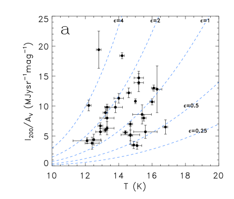
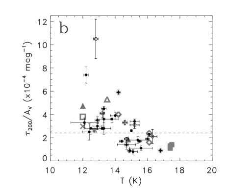
Figure 2: (a) Relationship between I₂₀₀/A_V and the dust temperature. Dashed lines represent iso-emissivity ($\epsilon$ =[$\tau_{200}$/A_V]/[$\tau_{200}$/A_V]_DISM = constant) curves. The corresponding emissivity values are indicated. (b) Relationship between the 200 $\mu$m emissivity ($\tau_{200}$/A_V) and the dust colour temperature. Black dots with error bars mark the fields investigated in this study. Open circles with error bars mark the reprocessed del Burgo et al. (2003) target fields. We also present recent results published in other papers, marked by gray symbols: – filled triangles: Stepnik et al. (2003); – filled, upside-down triangle: Pagani et al. (2003); – filled squares: Rawlings et al. (2005); – cross: Bianchi et al. (2003); – open triangle: Lehtinen et al. (1998); – open diamonds: Lehtinen et al. (2004); – open square: Juvela et al. (2002).

4 Uncertainties in the computation of emissivity parameters

The reliability of the final emissivity values derived for our target fields may be effected by several sources of errors. This is specially true, if a certain source of error does not contribute only to the random scatter of the derived values, but causes a certain pattern, which may be mistaken for a physical change in dust properties. In this section we investigate several potential error sources, and try to estimate their impact on the final emissivity determination.

4.1 Derivation of the correct extinction value

The extinction value A_V depends on the wavelength regime and the method used to derive it. In Sect. 2.2 we compared the results from the USNO star count and the near-infrared NICER method and concluded that the latter one is more suitable for our study.

The presence of foreground stars may also have an effect on the derived visual extinction values. While in a low extinction part of the cloud most stars in the beam are background objects, towards the densest peaks the stellar sample in the beam may be dominated by foreground stars. As a result, the visual extinction in the densest parts can be underestimated, and the emissivity value overestimated. Since the foreground objects show low E(B-V) values, we minimized the bias they cause by using an outlier resistant method to calulate the average reddening value in each cell in the NICER method. However, all of our target clouds are nearby (closer than a few hundred parsecs) and are located at high Galactic latitudes (b $\geq$ 15°), therefore the contribution of foreground stars is negligible.

The extinction value may also depend on the size of the grid and whether it is of fixed or adaptive type grid. Calculation of extinction/reddening using an adaptive gridsize may significantly underestimate the extinction, especially in a cloud centre, due to a inhomogeneous distribution of stars in the cells. We therefore preferred to use a fixed gridsize in our analysis.

4.2 Dependency of R_V

The ratio of total over selective extinction R_V is found to be significantly higher in dense interstellar clouds than R_V in the diffuse ISM (Cardelli et al., 1989; Whittet et al., 2001). This change is a strong indicator that the optical properties of dust grains differ in dense regions. When we derived A_V from A_J by following the method of Lombardi & Alves (2001), we adopted R_V = 3.1, which is a value typical for the diffuse ISM and may not be representative for the regions we investigate.

Applying the empirical relationship between R_V and $\rm{A_{J}}/{A_{V}}$ as determined by Cardelli et al (1989), we find $\rm{A_{J}}/{A_{V}}$ = 0.282 and 0.334, for R_V = 3.1 and 5.5, respectively, implying that $A_{V}$ will decrease by 19% when increasing R_V from values representative of the diffuse ISM to dense lines of sight. The corresponding I₂₀₀/A_V and $\tau_{200}$/A_V values will increase accordingly by 19%. We infer that the uncertainty in the assumption of R_V = 3.1 in the determination of $A_{V}$ has a relatively minor implication on the values of the observables presented in this paper. The assumption may introduce an underestimation of at most 20% in both I₂₀₀/A_V and $\tau$/A_V.

4.3 Application of a different emissivity law

Assuming that the exponent of the emissivity law $\beta$ is close to 2 in the interstellar medium (Gezari et al. 1973, Draine & Lee, 1984, Boulanger et al., 1996), we adopted $\beta$=2 to derive T_d from the slope of the short (90, 100 or 120 $\mu$m) versus long (200 $\mu$m) wavelength scatter plots (Sect. 3.1). Based on balloon-borne submillimetre observations of a large number of ISM regions, Dupac et al. (2003) found that $\beta$ is not constant but depends on the dust temperature as $\beta(\rm T)\,=\,(0.4+0.008\cdot(\rm T/1\,\rm K))^{-1}$. We used this relationship to investigate the effect of possible changes in $\beta$ on our results. We calculated the new colour temperature from the I_short versus I₂₀₀ scatter diagrams using $\beta(T)$. From this temperature we obtained the modified values for $\tau_{200}$/A_V.

Figure 3: Displacement of $\tau$/A_V vs. T_d data points due to the effect of a temperature dependent $\beta$ (Dupac et al., 2003). The original emissivity values with $\beta$ = 2 are marked by filled circles. The stripes originating from these points indicate the change due to a different $\beta$.

In Fig. 3 we show the effect of $\beta(T)$ on the temperature versus emissivity relationship. The $\beta$ dependency tends to increase the temperature, but the change is small, only for temperatures higher than 15.5 K the variations are noticeable, more than 0.3 K but less than 0.5 K. Although the new temperature-dependence of $\beta$ cause a systematic change of the distribution of the measurements in Fig. 3, the effect is small with respect to the measurement uncertainties.

4.4 Presence of warm dust

IRAS related studies of the dense and diffuse ISM have shown that extended emission at 60 $\mu$m can be associated with dust in low density regions. In these regions the 100 $\mu$m emission is closely correlated with the 60 $\mu$m emission, suggesting that they trace the same dust component in the ISM. At higher densities the 60 $\mu$m emission becomes weak indicating the absence of grains giving rise to the 60 $\mu$m emission. The remaining 100 $\mu$m emission is a signature of a “cold” dust component at $T<$15 K. This observation is supported by the close correlation of the cold dust component with ¹³CO emission. The surface brightness measured at a wavelength of $\lambda$ $\approx$ 100$\mu$m may contain emission from both the cold and the “warm” (or low density) dust component. The warm component will affect the determination of the $I_{\nu}/I_{200}$ colour temperature, such that the temperatures will be overestimated due to the short wavelength emission component.

To determine the fraction of the cold component in our short wavelength ($\sim$100 $\mu$m) maps we analysed 60 and 100 $\mu$m maps of our regions obtained with IRAS/ISSA because in most fields there are no ISOPHOT observations at 60 $\mu$m. The amount of emission from the cold component at 100 $\mu$m towards a specific sky position can be calculated from the two IRAS bands:

$$I_{cold}=I_{100}-\theta\cdot I_{60}$$ (1)

where $\theta$ is the slope of a linear relationship fitted to the 60 vs. 100$\mu$m surface brightness correlation diagram in the outer parts of the cloud. The relative contribution of the cold dust component at 100 $\mu$m is estimated from the correlation between I_cold and the original I₁₀₀ surface brightness. The scatter diagram was fitted by a linear function, resulting in a slope $X_{100}$, which gives the ratio of the cold dust emission to total surface brightness at 100 $\mu$m. We find typical values of 0.7 $\leq$ $X_{100}$ $\leq$ 0.8. We used $X_{100}$ to determine the cold dust emission contribution in the ISOPHOT short wavelength bands. Since the ISOPHOT measurements were not always taken at 100 $\mu$m, we converted $X_{100}$ to $X_{\lambda}$ assuming that the spectral energy distribution of the total surface brightness can be approximated by two modified black-bodies ($\beta$ = 2) with two different temperatures, T_warm and T_cold. We fixed T_warm to 17.5K (Lagache et al., 1998) and set T_cold to the temperature obtained from the original surface brightness scatter plots. Our analysis shows that $X_{\lambda}$/$X_{100}$ is close to 1 and the ratio is not very sensitive to T_cold. These $X_{\lambda}$ values were applied to the short wavelength surface brightness values at 90, 100 or 120 $\mu$m, to compute the corrected $\tau_{200}$/A_V values. The results are presented in Fig. 4.

Figure 4: Displacement of the T_d–$\tau_{200}$/A_V data points with the correction for the warm dust component of the short wavelength surface brightness values. The original data points are marked by filled circles and the stripes originating from them indicate the change due to the correction for the presence of warm dust.

Fig. 4 shows that the presence of warm dust tends to overestimate the temperature by 0.5–1 K which is significant. As a result, due to the lower temperature of the cold dust and since $I_{200}$/A_V is hardly affected, correction for warm dust emission increases warm dust increases $\tau_{200}$/A_V by at most $30$%.

4.5 Effect of surface brightness calibration errors

Figure 5: Effect of calibration errors in the surface brightness calibration. (a) Statistical errors in the short and long wavelength surface brightness (see the text for details). The four lines originating from each black dot (the original $\tau_{200}$/A_V data points) span a banana-shape area in the figure, corresponding to 9% calibration errors in both the short and long wavelength ISOPHOT surface brightness values, as found in Appendix A. (b) Displacement of the $\tau_{200}$/A_V values (stripes) relative to the original ones (black dots, as listed in Table 1), when the correlation coefficient between the ISOPHOT and DIRBE surface brightness calibration (see Appendix A) are applied.

Errors in the ISOPHOT surface brightness calibration may affect the derived dust temperatures and the relationships presented in Fig. 2. Here we first discuss the general effect of surface brightness calibration errors applying a simple model in Sect. 4.5.1.

Actual calibrational errors in this photometric system can only be unraveled by a comparison with a standard system. Due to its measurement design the DIRBE instrument on-board the COBE satellite was able to perform accurate absolute photometric observations (Hauser et al. 1998a) and serves now as the standard system for infrared sky brightness observations. A detailed comparison of the surface brightness photometric systems of ISOPHOT and that of COBE/DIRBE is presented in Appendix A. In Sect. 4.5.2 we apply the ISOPHOT–DIRBE surface brightness transformation equations found in Appendix A, and discuss their effect on our results.

4.5.1 General effect of calibration errors

In order to test the effect of the surface brightness calibration errors on the derived emissivities, in a simple approach we assumed a linear relationship between the true sky brightness and the surface brightness measured by a specific instrument/filter, i.e. the transformation equation between the two can be written as:

$$\mathrm{I}_{\lambda}^{\rm meas}\,=\,{\rm G_{\lambda}}{\times}I_{\lambda}^{\rm sky}+{\rm C_{\lambda}}$$ (2)

where I${}_{\lambda}^{\rm meas}$ is the measured sky brightness, I${}_{\lambda}^{\rm true}$ is the real sky brightness, and G (gain) and C (offset) are the coefficients describing the transformation.

Our analysis method, which is based on slope fitting in scatter plots (see Sect. 2), is not sensitive to errors due to constant offsets in the surface brightness. Multiplicative errors, however, change both the colour temperature and the emissivity parameters. Such errors may come from the presence of a gain uncertainty due to incorrect surface brightness calibration. We investigated the impact of this effect on our emissivity values, using a simple model. We assumed that I${}_{\rm short}^{\rm meas}$ = G${}_{\rm short}\cdot$I${}_{\rm short}^{\rm sky}$ and I${}_{200}^{\rm meas}$ = G${}_{200}\cdot$I${}_{200}^{\rm sky}$, where I${}_{\rm short}^{\rm sky}$ and I${}_{200}^{\rm sky}$ are the true surface brightness values of the sky at our short wavelength (either 90, 100 or 120 $\mu$m) and at 200 $\mu$m, respectively, while I${}_{\rm short}^{\rm meas}$ and I${}_{200}^{\rm meas}$ are the values affected by calibration errors. G_short and G₂₀₀ are the detector gains for the short wavelength and for the 200 $\mu$m filters, respectively. For both G_short and G₂₀₀ we assumed two extrema, 0.91 and 1.09, correspondig to an uncertainty value of 9%, as found for the ISOPHOT filters in Appendix A.

The effect of the four gain combinations for the derived emissivity values and dust temperatures is presented in Fig. 5a. The shorter, fully vertical lines originated from the black dots correspond to the cases, where both G_short and G₂₀₀ have the same value (either the same 0.91 or 1.09). In these cases the changes in the $\tau_{200}$/A_V values are 9%.

The longer, tilted lines correspond to the cases, when G_short and G₂₀₀ have opposite values. Then the amount of change in $\tau_{200}$/A_V and T_d depends noticeably on the original temperature, but in general is 25…30%. This is a major effect, but the $\tau_{200}$/A_V values remain in the domain, that their relative deviations from the emissivity of the diffuse interstellar matter is still significant.

The difference between the original and recalcultated dust temperatures are in the order of $\sim$0.7 K. As discussed in Sect. 3.1 these calibration errors are the main sources of uncertainty in the temperature determination.

The scenario presented here is indeed a ’worst-case’, i.e. the relative effect of the calibration errors at the two wavelengths are the strongest. The likely effect is smaller and would result in a final $\tau_{200}$/A_V uncertainty of 10…20%, depending on the original colour temperature. Here we also did not take into account the systematic calibrational differences between the two photometric systems, which could significantly reduce the final $\tau_{200}$/A_V uncertainties (see Sect. 4.5.2).

4.5.2 Effect of transformation between the ISOPHOT and COBE/DIRBE surface brightness photometric systems

We tested the effect of the correction of ISOPHOT surface brightness values by the ISOPHOT–DIRBE transformation coefficients found in Appendix A (see Table 2). Both the dust temperatures and the I₂₀₀/A_V ratios have been recalculated by the corrected surface brightness values in order to obtain the corrected $\tau_{200}$/A_V emissivities. The results are shown in Fig. 5b. The effect of this correction is small for the $\tau_{200}$/A_V values obtained from measurements with the 90 and 120 $\mu$m ISOPHOT filters. The 100 $\mu$m-related data points are more displaced, due to the relatively large difference in the scaling factors. However, the overall shape of the distribution did not change significantly, and the effect is much smaller than that of the general calibration errors presented in Sect. 4.5.1.

4.6 The impact of various error sources on the emissivity – dust temperature relationship

The distribution of data points in Fig. 2b indicates a clear trend in the $\tau_{200}$/A_V versus $T$ relationship: $\tau_{200}$/A_V is enhanced for T $<$ 14 K and decreases towards higher temperatures in the range 14 $\leq$ T $\leq$ 16 K. In the preceeding subsections we investigated possible mechanisms which could explain this observation, our findings are summarized below:

• 2MASS data provide reliable extinction maps for our regions. Contamination by foreground stars – which is most critical towards the densest regions – cannot be excluded, but probably has a minor effect.

• The dense clouds in our sample, presumably also the cold ones, may have a ratio of total over selective extinction R_V higher than the standard value of 3.1. As a consequence A_V may decrease at most by $\sim$19%, and the corresponding I₂₀₀/A_V and $\tau_{200}$/A_V values increase accordingly by the same fraction. However, high R_V should be restriced to small areas in our target fields. These regions are probably excluded anyhow due to their too low star count or too high extinction values (A_V $\geq$ 8 mag). Therefore the likely effect of R_V on the final emissivity values is below $\sim$10%.

• Assuming a temperature dependent emissivity law $\beta(T)$ instead of a fixed $\beta$ = 2 has a minor effect on the $\tau_{200}$/A_V distribution (Fig. 3). The differences with $\beta$ = 2 are more prominent at higher temperatures, but the main trend for clouds colder than the dust in the DISM is not changed.

• The possible presence of warm dust causes an overestimate of the dust temperature and, consequently, an underestimate of $\tau_{200}$/A_V by 10–30%. This variation is within the typical measurement uncertainties of the data points and does not alter the trend as observed in Fig. 2.

• Calibration errors can significantly modify the $\tau_{200}$/A_V and dust temperature values. The application of ISOPHOT surface brightness values corrected for the systematic differences of the ISOPHOT and COBE/DIRBE surface brightness photometric systems does not change the observed distribution of $\tau_{200}$/A_V values significantly. Applying a $\pm$9% general calibration uncertainty would cause a much severe effect, but the corrected results remain in the $\sim$25% range to the original values. Transformation of the ISOPHOT surface brightness values to the DIRBE photometric system has only a minor effect on the T_d vs. $\tau_{200}$/A_V relationship.

From the uncertainties due to different error sources we estimated a general $\sim$30% uncertainty for our $\tau_{200}$/A_V values. To match the observations by assuming a constant emissivity (that of the DISM) a 50…80% uncertainty is required, which is unrealistic, according to our investigations. The observed temperature versus $\tau_{200}$/A_V relationship, as presented in Fig. 2b, most probably indicates physical changes and is not due to artifacts in the data or to incorrect initial assumptions in the calculations.

5 Discussion

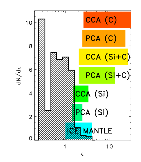
Figure 6: The histogram with shaded area shows the relative frequency ($dN/d\epsilon$) of the observed $\tau_{200}$/A_V values relative to that of the DISM ($\epsilon$ = $\tau_{200}$/A_V/[$\tau_{200}$/A_V]_DISM, where [$\tau_{200}$/A_V]_DISM = 2.4$\cdot$10^-4 mag^-1), found for our targets. Horizontal bars represent the predicted range of enhancement in emissivity for different types of grains following Stognienko et al. (1995), from bottom to top: (1) ice mantles, (2) silicate particle-cluster aggregates, (3) silicate cluster-cluster aggregates, (4) mixed (silicate and carbon) particle-cluster aggregates, (5) mixed cluster-cluster aggregates, (6) carbon particle-cluster aggregates (7) carbon cluster-cluster aggregates.

5.1 Observed variations in $\tau_{200}$/A_V

We found notable differences between the original del Burgo et al. (2003) $\tau_{200}$/A_V values and the emissivities of the same fields reprocessed in this paper. The main differences between our and the del Burgo et al. (2003) processing are that in this study we applied extinction values derived from 2MASS data and that we used different short wavelength data for the temperature calculation, namely 90, 100 or 120 $\mu$m instead of 150 $\mu$m (these new results are also included in Table 1 and in Fig. 2). The dust temperatures we found are consistent with those in del Burgo et al. (2003). However, the resulting I₂₀₀/A_V ratios are different, and this discrepancy lead to notably lower $\tau_{200}$/A_V values (see Table 1). This also indicates, that it is mainly the application of 2MASS data that is responsible for the differences seen in the emissivities.

Our values obtained for the TMC 2 (G173.9–15.7 and G174.3–15.9) and for LDN 1780 (G359.1+36.7) are very similar to the average values presented for these clouds by del Burgo & Laureijs (2005) and Ridderstad et al. (2006), respectively. In these papers I₂₀₀/A_V and $\tau_{200}$/A_V values were derived by taking the brightness ratios from the maps instead of correlation plots. Despite the general argeement with our data, the detailed analysis of LDN 1780 show that $\tau_{200}$/A_V can range from 10⁴ mag^-1 to 4$\cdot$10⁴ mag^-1 within the same cloud (Ridderstad et al., 2006). An even higher increase of $\tau_{200}$/A_V is observed in the Taurus 2 molecular cloud (del Burgo & Laureijs, 2005).

An important outcome of our analysis of a large sample of cloud regions is that we find a clear trend of $\tau_{200}$/A_V versus $T_{\rm d}$, but that the variation in $\tau_{200}$/A_V is less pronounced than initially reported by other studies. Only three fields exhibit $\tau_{200}$/A_V which is more than threefold the value for the DISM ($\tau_{200}$/A_VDISM). All other regions with $T_{\rm d}<$14 K (12 regions) have $\tau_{200}$/A_V $>$ $\tau_{200}$/A_VDISM. In the majority of the regions with $T_{\rm d}>$14 K the emissivities are below $\tau_{200}$/A_VDISM (10 out of 12 regions). One extreme case is G142.0+38.5, where 3$\tau_{200}$/A_V $\approx$ $\tau_{200}$/A_VDISM.

The values of $\tau_{200}$/A_V in our sample refer to the average properties (T_d, and I₂₀₀/A_V) over a relatively extended region of $\sim$100 arcmin². The enhancement observed by us of $\epsilon<2$ in most cases suggests, that higher $\epsilon$ values usually occur only in smaller regions inside the clouds, possibly in the densest cores.

We have not seen large deviations in the scatter plots, neither in the I₂₀₀/A_V, nor in the dust temperature derivation, as reflected in the uncertanties in T_d and I₂₀₀/A_V. Extremely high, local emissivities are expected to show up in these scatter plots, and are therefore excludeable in our fields at the resolution we adopted, namely 3$\aas@@fstack{\prime}$5.

5.2 Changes of dust properties at low temperature

Below 14 K all $\tau_{200}$/A_V values are higher than 2.4$\cdot$10^-4 mag^-1, the representative value of the DISM. This finding agrees with the results of several earlier papers (see Sect. 1 and the caption of Fig. 2). The majority of our data points are within a well-defined range, 1-to-2 times the emissivity of the DISM. Enhanced emissivity values are usually interpreted as the change of dust properties: coagulation of dust particles or formation of ice mantles on grain surfaces (see e.g. Dwek 1997). Dust grains may show a large variety both in composition (silicate, carbon, or mixed) and in structure (ice mantle, particle-cluster aggregates, cluster-cluster aggregates) and the different types show different enhancement of the emissivity. Since the emissivity enhancement typically is not higher than a factor of 2, our results are consistent with ice mantles or cluster of silicate particles (CCA or PCA, see Fig. 6). On the other hand far-infrared emissivities produced by grains containting carbon aggregates are too high for most of our observed emissivity values. However, in some particular regions the observed $\tau_{200}$/A_V exceeds significantly the representative values of the DISM, and may indicate the existence of carbonaceous grains.

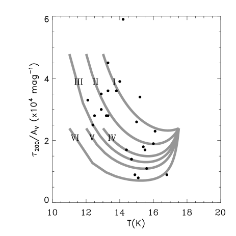
Figure 7: In this figure we present model fits of T_d versus $\tau_{200}$/A_V with a dust emission of bimodal temperature distribution. The gray curves represent different emissivities and cold temperatures (T_c). To derive the ”virtual” dust temperature, surface brightness at 100 $\mu$m (short) and 200 $\mu$m (long) wavelengths were used. The warm dust temperature has been set to T_w = 17.5 K. Other short wavelengths (90 or 120 $\mu$) produce curves very close to the 100 $\mu$m ones. I. $\epsilon$ = 2.0, T_c = 13.0 K; II. $\epsilon$ = 2.0, T_c = 12.0 K; III. $\epsilon$ = 2.0, T_c = 11.0 K; IV. $\epsilon$ = 1.0, T_c = 13.0 K; V. $\epsilon$ = 1.0, T_c = 12.0 K; VI. $\epsilon$ = 1.0, T_c = 11.0 K; The black dots mark our measured $\tau_{200}$/A_V values.

5.3 Emissivities lower than in the DISM

As presented in Sect. 3.3 and Fig. 2, we find low emissivity values for 14 K $\leq$ T_d $\leq$ 16 K colour temperatures. Similar results were obtained for some specific regions by Lehtinen et al. (2004) and by Rawlings et al. (2005). Even though one can explain an emissivity lower than that of the DISM in terms of changed grain properties, it is also possible to explain this behaviour using a bimodal temperature model (Cambresy et al., 2001; del Burgo et al., 2003). In this model we assume, that the observed far-infrared surface brightness is due to two emission components with different dust temperatures, both due to big grains. The observed infrared emission can be written as:

$$I_{\nu}=\tau_{\nu,c}B_{\nu}(T_{\rm c})+\tau_{\nu,w}B_{\nu}(T_{\rm w})$$ (3)

where T_c and $T_{\rm w}$ are the temperatures of the cold and warm dust components, respectively, and $\tau_{\nu,c}$ and $\tau_{\nu,w}$ are the infrared optical depths of the cold and warm components, respectively. The emissivity of the cold component may differ from that of the warm component, and this change is characterized by the $\epsilon$ parameter:

$$\tau_{\nu,c}=\epsilon X\tau_{\nu,tot}$$ (4)

$$\tau_{\nu,w}=(1-X)\tau_{\nu,tot}$$ (5)

where $\tau_{\nu,tot}$ is the total effective optical depth if both components had identical emission properties and X is the fraction of the optical depth of the cold component with respect to the effective total opacity (for more details see del Burgo et al. 2003). In del Burgo et al. (2003) the cold temperature T_c was choosen to be 13.5 K, representing the lowest colour temperatures obtained from their sample. However, in our sample we included denser molecular regions and the presence of colour temperatures of T_d $\approx$ 12 K obviously requires a lower T_c value.

We derived the colour temperature from the slope of the scatter plot of two IR-wavelength surface brightness distributions. It is easy to see that in a bimodal temperature distribution the variation of X causes a change in the ratio of surface brightness values measured at two wavelengths (see Fig. 8 in del Burgo et al., 2003), i.e. an effect very similar to the change of the colour temperature. A specific X value can be directly linked to a “virtual” colour temperature, as long as $T_{\rm c}$ and $T_{\rm w}$ are fixed. As we demonstrate below, mixing rather than change of dust grain properties can be the reason that data points in Fig. 2b fall below the representative value of the DISM. In Fig. 7 we plot $\tau_{200}$/A_V model curves with mixing ratios changing in the 0 $\leq$ X $\leq$ 1 range, versus the corresponding virtual colour temperature. In this model we used $\tau_{\nu,tot}$ = 2.4$\cdot$10^-4 mag^-1, which is the representative value of the DISM (Schegel et al., 1998). In all cases we kept T_w = 17.5 K and assumed different values of T_c. For $\epsilon$ either $\epsilon$ = 1 or $\epsilon$ = 2 was adopted.

It is clear from Fig. 7, that in order to reproduce the higher $\tau_{200}$/A_V values for cold regions (T $<$ 14K) the emissivity of the cold component in the bimodal model has to be enhanced.

It is noteworthy, however, that the observed low $\tau_{200}$/A_V values (14K $\leq$ T $\leq$ 16K), can be well fitted by using $\epsilon=1$ for both the warm and cold components.

This result suggests that the presence of colder component with the same grain properties as for the DISM is sufficient to explain the low $\tau_{200}$/A_V in a region. The most plausible reason is that radiative transfer in these regions can cause some parts to become colder while our temperature measurement is biased towards the warmer regions. However, a necessary condition is that the colder component is well mixed and not resolved by ISOPHOT, otherwise the scatter diagrams would become highly non-linear. Whether this can be achieved in a cloud model, needs to be investigated.

5.4 Smaller grains

An alternative explanation for low emissivity clouds with low column density is an enhancement of the relative contribution of small grains, since for a grain size $a$, $Q_{abs}\,{\propto}\,a$ in the far-infrared. If this is a likely mechanism then the regions with $\tau_{200}$/A_V lower than the DISM would have undergone some recent processing such that the relative amount of small grains is larger than in the standard grain size distribution. We note that a fraction of the clouds were selected from the IRAS data on the basis of the high 100 $\mu$m brightness. These clouds also exhibit a high brightness in the IRAS 12, 25, and 60 $\mu$m bands and could indicate a bias towards clouds with a grain size distibution favouring the smaller sizes.

6 Conclusions

In this paper we have analysed the FIR emission properties in a large sample of interstellar clouds, observed with ISOPHOT. We have derived far-infrared emissivity relative to the visual extinction, $\tau_{200}$/A_V, for each region. The derived values of $\tau_{200}$/A_V represent the average emissivity over a region typically in the order of 100 arcmin².

The derived FIR emissivities $\tau_{200}$/A_V show an enhancement for the coldest and densest regions where 12 K $\leq$ T_d $\leq$ 14 K, which is most probably due to the growth of dust grains. We confirm a similar trend found in earlier papers. The enhancement of $\tau_{200}$/A_V for 12 K $\leq$ T_d $\leq$ 14 K is for the majority of the regions less than 2. This is lower than previously reported for some specific clouds. Our findings support models where the enhancement in emissivity is attributed to ice mantle growth and the presence of silicate agregrates on the spatial scales we investigated.

For 14 K $\leq$ T_d $\leq$ 17.5 K, we observe a majority of regions where $\tau_{200}$/A_V is lower than that of the diffuse ISM. FIR emissivities lower than that of the DISM may be explained by the common effect of a constant emissivity and the presence of multiple dust temperatures along the line of sight. To sufficiently fit the observed values the cold temperatures (T_c) had to be set to $\sim$12K without significantly altering the dust properties. Alternatively, these clouds in our sample could be biased towards regions with a more significant small grain component in their dust size distribution.

7 Acknowledgments

We thank the referee Dr. Mika Juvela for detailed comments and suggestions which helped us to improve the manuscript. This paper is based on observations with ISO an ESA project with instruments funded by ESA member states (especially the PI countries: France, Germany, the Netherlands and the United Kingdom) and with participation of ISAS and NASA. The ISOPHOT data were processed using PIA, a joint development by the ESA Astrophysics Division and the ISOPHOT consortium led by MPI für Astronomie, Heidelberg. Contributing Institutes are DIAS, RAL, AIP, MPIK, and MPIA.

This research has made use of the following catalogues/services:

• USNOFS Image and Catalogue Archive, operated by the United States Naval Observatory, Flagstaff Station (http://www.nofs.navy.mil/data/fchpix/)

• NASA/IPAC Infrared Science Archive, which is operated by the Jet Propulsion Laboratory, California Institute of Technology, under contract with the National Aeronautics and Space Administration (the 2MASS point source catalogue)

• ISO Data Archive, European Space Astronomy Centre of the European Space Agency (http://www.iso.esac.esa.int/ida/)

This research has been supported by the grants T34584 and K62304 of the Hungarian Research Fund.

Appendix A Comparison of the ISOPHOT and COBE/DIRBE surface brightness photometric systems

The calibrational accuracy of the ISOPHOT surface brightness photometric system is crucial for the interpretation of the final results. Due to the lack of proper extended standard objects on the sky, especially at far-infrared wavelengths, the only practical possibility to test the accuracy is a comparison of ISOPHOT data with that of COBE/DIRBE values. Here first we check the general relationship of the ISOPHOT and COBE/DIRBE surface brightness systems via the comparison of P22 mini-map highly processed data product (HPDP) background values from the ISO Data Archive. In a second approach average surface brightness values of our target fields of the present study, obtained from ISOHPOT observations is compared with those derived from COBE/DIRBE surface brightness data.

A.1 Description of the COBE/DIRBE background determination

The monochromatic COBE/DIRBE surface brightness value at a specific wavelength, date and sky position is derived with the PredictDIRBE tool, written in IDL and developed in Konkoly Observatory, using some routines written at Max-Planck-Institut für Astronomie, Heidelberg. The PredictDIRBE routine uses the CGIS software library, developed to help the analysis of COBE data. PredictDIRBE uses two main DIRBE data products, the DIRBE sky and zodi atlases (DSZA) and the zodi-subtracted mission average maps (ZSMA). The detailed description of these DIRBE data products can be found on the COBE/DIRBE homepage of IPAC. The main steps of the COBE/DIRBE surface brightness determination in the PredictDIRBE routine are the following:

• Extraction of DIRBE ZSMA (zodiacal light component removed) surface brightness values for the 10 DIRBE photometric bands. The number of DIRBE pixels considered here as well as for the determination of the zodiacal contribution depends on the extension of ISOPHOT maps. However, the spatial sampling of DIRBE measurements at long wavelenghts is very fine relative to the physical resolution ($\sim$30′or worse). The operations below are done for the median values of the DIRBE pixels taken.

• Colour correction of the cirrus component. In this step the temperature of the cirrus component is derermined by fitting the 100, 140 and 240 $\mu$m ZSMA surface brightness values with a modified black-body spectral energy distribution (SED), I_ν $\propto$ $\nu^{\beta}$B${}_{\nu}\rm(T)$, where B${}_{\nu}\rm(T)$ is the Planck-function at temperature T and frequency $\nu$, and $\beta$ is the spectral index. The 140 $\mu$m DIRBE band has a lower weight in the fitting process, due to its well-known noisy behaviour compared to the other bands. For our calculations the spectral index has been fixed to $\beta$ = 2. For $\lambda$ $<$ 100 $\mu$m the SED is approximated by a function fitted by spline interpolation to the measured log$(\lambda)$ – log(I${}_{\lambda}^{\rm DIRBE})$ values. The colour correction is performed using the fitted SEDs, and the transmission curves of the DIRBE filters. The final, monochromatic surface brightness values are reached by the repetition of this process, until the convergence criterium is matched. We have to note, that the ZSMA surface brightness contains at least two main components: the cirrus (or, in general Galactic interstellar matter) emission and the extragalactic background. Although the two components have different SEDs, the difference between colour corrections needed for the two different SEDs is small, and in most cases the absolute level of the extragalactic background component is much below that of the cirrus. Therefore here we do not consider these two components separately.

• Determination of the non-zodiacal DIRBE surface brightness at the ISOPHOT wavelength. The monochromatic DIRBE surface brightness values are interpolated to the nominal ISOPHOT filter wavelength. For $\lambda$ $<$ 100 $\mu$m this is performed by the spline interpolation of the log$(\lambda)$ – log(I${}_{\lambda}^{\rm DIRBE})$ values, while for $\lambda$ $\geq$ 100 $\mu$m the previously mentioned $\nu^{\beta}$B${}_{\nu}\rm(T)$ is applied.

• The zodiacal component is determined from the DIRBE zodi atlases (DSZA products). From the date of the observation the actual solar elongation angle of the requested sky coordinate is calculated. In case no DIRBE observation was performed at that solar elongation and ecliptic latitude (due to the limited lifetime of the instrument), the actual solar elongation is ”mirrored”, so that the solar elongation with the same absolute value is taken on the other side of the Sun, and the zodiacal component is extracted at the corresponding dates and coordinates. This latter position was in almost all cases observed by DIRBE (for the details of COBE/DIRBE observations, see Hauser et al., 1998b). The zodiacal component is extracted for all the 10 DIRBE photometric bands.

• Colour correction of the zodiacal component is performed assuming a pure black-body SED around the peak of the zodiacal emission, and using spline interpolation for notably shorter and longer wavelengths, applying otherwise the same iterative process as for the colour correction of the non-zodi component above. The resulting monochromatic zodiacal surface brightness values are used to interpolate to the requested ISOPHOT wavelength.

• The final PredictDIRBE surface brightness is the sum of the monochromatic zodiacal and the non-zodiacal (cirrus + extragalactic background) components.

A.2 Minimaps HPDPs

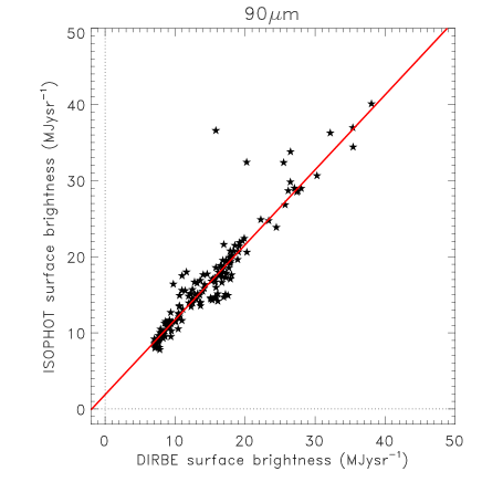
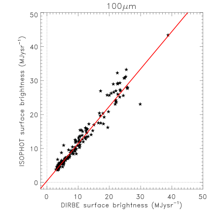
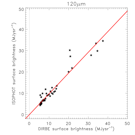
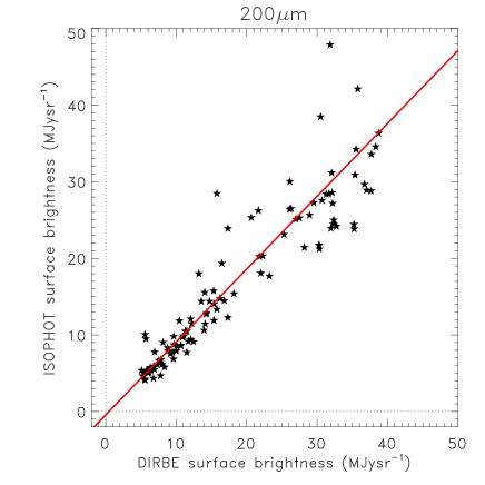
Figure 8: Comparison of minimap background surface brightness values and background estimates based on COBE/DIRBE data at different wavelengths (a) 90 $\mu$m, (b) 100 $\mu$m, (c) 120 $\mu$m and (d) 200 $\mu$m. The solid lines are fitted linears, corresponding to the values in Table 2.

Mini-map mode was a ’submode’ of the P22 astronomical observing template (AOT, see Laureijs et al. 2003) of ISOPHOT. The mode was especially designed to obtain accurate fluxes of point/compact sources. However, apart from the point source flux determination, the mini-maps provide accurate surface brightness values of the average background around the target, due to the redundant observation of the same sky position by many ISOPHOT pixels. The mini-map backgrounds are assumed to be homogeneous for the whole mini-map area. The typical spatial extension of a minimap is $\sim$4′  for both the C100 and the C200 detector arrays.

The background values can be compared with the values obtained by the PredictDIRBE routine for the specific central coordinates of the source (assuming a 30′ aperture) and for the ISOPHOT wavelengths. Moór et al. (2003, 2004a, 2004b and 2005) performed a full re-evaluation of a large sample of ISOPHOT mini-maps, containing the observations of normal stars, evolved stars, extragalactic and miscellaneous objects. The publicly available ISO Data Archive contains the re-evaluated results of these observation as Highly Processed Data Products (Salama et al., 2004).

The results of the COBE/DIRBE and mini-map background comparisons are presented in Fig. 8 for the four ISOPHOT filters used in our study (90, 100, 120 and 200 $\mu$m). In Table 2 we present the coefficients found for the correlation between the DIRBE and ISOPHOT surface brightness photometric systems, assuming the linear relationship

$$\mathrm{I}_{\lambda}^{\rm ISOPHOT}\,=\,{\rm S}{\times}I_{\lambda}^{\rm DIRBE}+{\rm Offset}$$ (6)

where I${}_{\lambda}^{\rm ISOPHOT}$ and I${}_{\lambda}^{\rm DIRBE}$ are the surface brightness values at the wavelength $\lambda$, measured with ISOPHOT and DIRBE, respectively.

$\lambda$	S	Offset	R1:1	Rf
($\mu$m)		(MJy sr-1)	(%)	(%)
90	0.98($\pm$0.02)	1.87($\pm$0.13)	14.2	8.5
100	1.09($\pm$0.03)	0.43($\pm$0.13)	16.7	10.5
120	0.97($\pm$0.06)	0.02($\pm$0.28)	12.8	11.4
200	0.95($\pm$0.03)	–0.44($\pm$0.24)	14.9	10.8

Table 2: Parameters describing the relation between the DIRBE and ISOPHOT surface brightness photometric systems, derived from the mini-map HPDP sample, assuming a linear relationship. The columns of the table are: (1) ISOPHOT filter nominal wavelength; (2) fitted scaling factor (S), assuming Eq. 6; (3) fitted offset, assuming Eq. 6; (4) mean relative deviation of original ISOPHOT and DIRBE surface brightness values; (5) mean relative deviation of ISOPHOT and DIRBE surface brightness values after the correction with the fitted line;

The last two columns of Table 2 contain the mean relative deviations of orignal ISOPHOT and DIRBE surface brightness values (column #4) and the mean relative deviations of the original ISOPHOT and DIRBE surface brightness values after the correction with the fitted line (’residual scatter’, column #5). These values are representative for the general relative accuracy of the two photometric systems.

The DIRBE surface brightness calibration (as well as that of ISOPHOT) contains intrinsic uncertainties, both in detector gain and offset. These uncertainties contribute significantly to the observed relative deviations listed in Table 2. For those DIRBE filters that are important for the comparison with the ISOPHOT surface brightness calibration in this paper, the typical gain uncertainties are 13.5%, 10.6% and 11.6% for the 100, 140 and 240 $\mu$m DIRBE bands, respectively (see Arendt et al., 1998). These DIRBE gain uncertainties indicate the presence of an additional uncertainty in the order of $\sim$10% or below, which should account for the uncertainties in the PredictDIRBE estimate calculation as well as in the intrinsic uncertainties of the ISOPHOT calibration.

The typical offset uncertainties are 0.3, 0.6 and 0.4 MJy sr^-1 for the 100, 140 and 240 $\mu$m DIRBE bands per pixel, respectively (Arendt et al., 1998). These are in the order of the offset values found for the ISOPHOT–DIRBE comparison (see Table 2), except for the 90 $\mu$m ISOPHOT filter, where this offset is significantly higher. However, the 90 $\mu$m surface brightness values may also contain an emission contribution from a grain population different from the one responsible for the $\lambda$ $\geq$ 100 $\mu$m part of the background SED. This effect is not accounted for in the PredictDIRBE routine.

In the case of ISOPHOT, non-unity scaling factors may arise from imperfect knowledge of the effective solid angles at different wavelengths and/or from a flux-dependent non-linearity of the detector. ISOPHOT solid angles have been re-assessed recently (Ábrahám et al. 2005, ISOPHOT internal calibration report) and the new values agree within 5% with the previous ones. Non-linearity can occur due to calibration uncertainties in the extrapolation to weak flux levels because the ISOPHOT calibration targets were always much brighter than the ISM in the ISOPHOT beams. The importance of the non-linearity can be estimated via comparison with the COBE/DIRBE calibration. According to the results presented in Table 2 the relationships between the ISOPHOT and COBE/DIRBE surface brightness values are sufficiently linear.

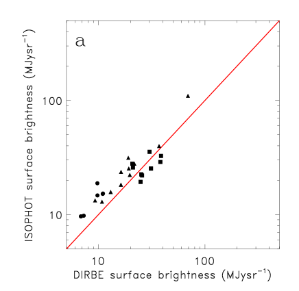
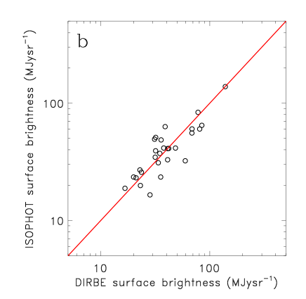
Figure 9: Comparison of the average surface brightness of our target fields and the DIRBE surface brightness derived for the same sky positions and observational dates, with the PredictDIRBE routine. (a) Short wavelength filters (ISOPHOT 90, 100 and 120 $\mu$m, marked by filled circles, triangles and squares, respectively); (b) ISOPHOT 200 $\mu$m filter. The solid lines mark the 1:1 line.

A.3 Fields of the present study

The target fields of the present study were observed by the same AOT (P22) as the mini-maps, with some notable differences between the two samples. First, the extension of the target field maps is in the 5′…40′range, while the mini-maps are smaller than these. Second, the intensity of the target maps contains the contribution of point sources and also that of larger scale structures, while the point source emission was subtracted in the derivation of the mini-map backgrounds.

The average surface brightness of our target fields were derived as simple average of all pixel values, for both the short and the long wavelength maps of a specific field. PredictDIRBE estimates of the DIRBE surface brightness were calculated for the central positions of the ISOPHOT maps. The observational date of the maps were also considered to account for the annual variation of the zodiacal light component. The results are presented in Fig. 9 and in Table 3.

field	$\lambda_{s}$/$\lambda_{l}$	I${}_{s}^{D}$	I${}_{s}^{PHT}$	I${}_{l}^{D}$	I${}_{l}^{PHT}$
G004.3+35.8	100 / 200	19.0	31.5	38.9	63.1
G100.0+14.8	90 / 200	11.0	15.3	31.5	34.6
G101.8+17.0	100 / 200	10.8	13.0	23.1	19.9
G102.0+15.2	90 / 200	9.8	14.7	37.8	41.5
G114.0+14.9	120 / 200	24.8	19.3	41.0	32.9
G114.3+14.7	120 / 200	25.6	22.0	42.0	41.1
G114.6+14.6	120 / 200	25.2	22.5	41.0	41.0
G121.6+24.6	90 / 200	7.3	9.8	22.8	27.0
G122.0+24.2	90 / 200	6.8	9.6	21.1	23.1
G142.0+38.5	100 / 200	9.3	13.3	16.7	18.8
G170.2–16.0	120 / 200	31.1	25.3	48.4	41.4
G173.9–15.7	120 / 200	38.1	28.9	68.5	55.7
G174.3–15.9	120 / 200	38.6	32.6	68.7	60.3
G297.3–16.2	100 / 200	21.7	27.9	84.5	64.7
G300.2–16.8	120 / 200	9.8	18.8	31.8	39.2
G301.7–16.6	90 / 200	16.3	23.7	34.8	37.3
G302.6–15.9	100 / 200	13.0	15.8	28.3	16.5
G303.5–14.2	100 / 200	19.7	22.2	59.5	32.2
G303.8–14.2	100 / 200	16.2	18.3	35.4	23.5
G355.3+14.7	100 / 200	69.2	109.7	138.8	138.4
G359.1+36.7	100 / 200	19.2	25.3	23.6	25.8
G359.9–17.9	100 / 200	37.0	39.8	78.0	83.5
G089.0–41.2∗	90 / 200	11.0	15.2	20.0	23.5
G111.2+19.6∗	150 / 200	31.2	32.2	33.7	31.0
G187.3–16.7∗	120 / 200	30.2	35.4	35.8	48.6
G297.3–15.7∗	150 / 200	66.8	63.7	80.8	60.2
G301.2–16.5∗	120 / 200	20.8	27.9	31.1	49.3
G301.7–16.6∗	120 / 200	21.1	25.8	31.9	51.1

Table 3: The columns of the table are: (1) the name of the field (central galactic coordinates); (2) central wavelengths of the short/long ISOPHOT filters [$\mu$m/$\mu$m]; (3) short wavelength DIRBE surface brightness [MJy sr^-1]; (4) short wavelength ISOPHOT surface brightness [MJy sr^-1]; (5) long wavelength DIRBE surface brightness [MJy sr^-1]; (6) long wavelength ISOPHOT surface brightness [MJy sr^-1]

A.4 Summary

The results of the DIRBE and ISOPHOT surface brightness comparisons can be summarized as follows:

• In general a very good linear relationship was found between the ISOPHOT and DIRBE surface brightness photometric systems.

• The scaling factors between the DIRBE and the ISOPHOT surface brightness photometric systems are close to unity, within the uncertainties. Even largest difference (100 $\mu$m) is within 9% to the DIRBE system. These scaling factors indeed have an impact on the derived dust temperatures and I₂₀₀/A_V ratios. This effect is widely discussed for the typical deivations in the main text (see Sect. 4.5).

• The offsets found between the DIRBE and ISOPHOT surface brightness calibration based on the mini-map database are usually small (see Table 2). The largest offset value ($\sim$1.9 MJy sr^-1) is found for the ISOPHOT 90 $\mu$m filter. However, in this paper we applied the method of slope fitting in the derivation of dust temperature from surface brightness scatter plots and in the determination of the I₂₀₀/A_V ratio, which is completely insensitive for offsets.

• Not taking into account the systematic differences, the mean relative deviations between the ISOPHOT the COBE/DIRBE surface brightness values are within $\sim$15% for the four investigated wavelengths.

• The comparison of the ISOPHOT vs. DIRBE relative deviations with the DIRBE intrinsic detector gain uncertainties and the ISOPHOT vs. DIRBE offsets with the DIRBE intrinsic offset uncertainties show, that the uncertainties in the DIRBE surface brightness calibration have a siginificant impact on the ISOPHOT–DIRBE comparison. The DIRBE detector calibration uncertainties are at a similar level than other error sources (e.g. ISOPHOT detector calibration uncertainties, DIRBE background estimate uncertainties by the PredictDIRBE routine) and they may be dominant in some cases.

• A representative ISOPHOT calibration uncertainty can be estimated by subtracting the DIRBE detector gain uncertainties (in average $\sim$12% for the 100, 140 and 240 $\mu$m DIRBE bands) from the mean relative deviations between the two photometric systems (in average $\sim$15%, see column #4 in Table A1). The resulting value which we adopt for both short and long ISOPHOT wavelengths is 9%.

• The DIRBE and ISOPHOT surface brightness values in the target fields show a behaviour very similar to that of the mini-map backgrounds. The general agreement between the ISOPHOT and DIRBE surface brightness values are very good. The relatively large deviations in some cases may be explained by the beamsize of DIRBE, which is large, even compared to the size of the ISOPHOT target maps.

References

- Arendt et al. (1998) Arendt, R.G., Odegard, N., Weiland, J.L., et al., 1998, ApJ 508, 74
- Bernard et al. (1999) Bernard J. et al., 1999, A&A, 347,
- Bianchi et al. (2003) Bianchi S., Gon alves J., Albrecht M., Caselli P., Chini R., Galli D., Walmsley M. et al., 2003, A&A, 399, L43
- Boulanger et al. (1996) Boulanger F., Abergel A., Bernard J.-P., Burton W.B., Desert F.-X., Hartmann D., Lagache G., Puget J.-L., 1996, A&A, 312, 256
- del Burgo et al. (2003) del Burgo C., Laureijs R.J., Ábrahám P., Kiss Cs., MNRAS, 346, 403
- del Burgo et al. (2005) del Burgo C., Laureijs R.J., 2005, MNRAS, 360, 901
- Cambrésy et al. (1997) Cambrésy L., et al., 1997, A&A 324, L5
- Cambrésy et al. (2001) Cambrésy L., Boulanger F., Lagache G., Stepnik B., 2001, A&A, 375, 999
- Cambrésy et al. (2002) Cambrésy, L., Beichman, C.A., Jarrett, T.H., Cutri, R.M., 2002, AJ 123, 2559
- Cardelli et al. (1989) Cardelli J.A., Clayton G.C., Mathis, J.S., 1989, ApJ 345, 245
- Cutri et al. (2003) Cutri R.M., Skrutskie M.F., van Dyk, S., 2003, 2MASS All-Sky Catalog of Point Sources, VizieR On-line Data Catalog: II/246
- Draine & Lee (1984) Draine B.T., Lee H.M, 1984, ApJ, 285, 89
- Dupac et al. (2003) Dupac X. et al., 2003, A&A, 404, L11
- Dwek (1997) Dwek, E., 1997, ApJ, 484, 779
- Gabriel et al. (1997) Gabriel C., Acosta-Pulido J., Heinrichsen I., Morris H., Tai W.-M., 1997, in Hunt G., H. E. Payne, eds., Astronomical Data Analysis Software and Systems VI, A.S.P. Conference Series, Vol. 125, p. 108
- Gezari et al. (1973) Gezari D.Y., Joyce R.R., Simon M., 1973, ApJ, 179, L67
- Hauser et al. (1998a) Hauser, M.G., Arendt, R.G., Kelsall, T., 1998a, ApJ 508, 25
- Hauser et al. (1998b) Hauser, M.G., Kelsall, T., Weiland, J. (eds.), and the COBE Science Working Group, 1998b, ”COBE Diffuse Infrared Background Experiment (DIRBE) Explanatory Supplement”, Version 2.3 (14 January 1998), available on-line: http://lambda.gsfc.nasa.gov/product/cobe/dirbe_exsup.cfm
- Juvela et al. (2002) Juvela M., Mattila K., Lehtinen K., et al., 2002, A&A, 382, 583
- Kiss et al. (2006) Kiss, Z., Tóth, L.V., Krause, O., Kun, M., Stickel, M., 2006, A&A, 453, 923
- Klaas et al. (2003) Klaas U., et al., 2003, ”ISOPHOT In-flight Calibration Strategies”, in: ”The Calibration Legacy of the ISO mission”, ESA SP-481, p. 19
- Lada et al. (1994) Lada, C.J., Lada, E.A., Clemens, D.P., Bally, J., 1994, ApJ 429, 694
- Lagache et al. (1998) Lagache G., Abergel A., Boulanger F., Puget J.-L., 1998, A&A, 333, 709
- Laureijs et al. (2003) Laureijs R.J., Klaas U., Richards P.J., Schulz B., Ábrahám P., 2003, The ISO Handbook Vol. V.: PHT – The Imaging Photo-Polarimeter, Version 2.0.1, ESA SP-1262, European Space Agency
- Lehtinen et al. (1998) Lehtinen K., Lemke D., Mattila K., Haikala L.K., 1998, A&A, 333, 702
- Lehtinen et al. (2004) Lehtinen K., Russeil D., Juvela M., Mattila K., Lemke D., 2004, A&A, 423, 975
- Lemke et al. (1996) Lemke D., et al., 1996, A&A, 315, L64
- Lombardi & Alves (2001) Lombardi M., Alves J., 2001, A&A, 337, 1023
- Monet et al. (1998) Monet D.G., Bird A., Canzian B., 1998, The USNO-A2.0 Catalogue, VizieR On-line Data Catalog: I/252. Originally published in: U.S. Naval Observatory Flagstaff Station (USNOFS) and, Universities Space Research Association (USRA) stationed at USNOFS
- Monet et al. (2003) Monet D.G., Levine S.E., Canzian B., 2003, AJ, 125, 984
-
Moór et al. (2003)
Moór, A., Ábrahám, P., Kiss, Cs., Csizmadia, Sz., 2003,
Far-infrared observations of normal stars measured with ISOPHOT
in mini-map mode, report on Highly Processed Data Products, Version 1.1,
available on-line at the ISO Data Centre:
http://pma.iso.vilspa.esa.es:8080/hpdp/technical_reports/
technote38.html -
Moór et al. (2004)
Moór, A., Ábrahám, P., Kiss, Cs., Csizmadia, Sz., 2004a,
Far-infrared observations of evolved stars measured with ISOPHOT
in mini-map mode, report on Highly Processed Data Products, Version 1.0,
available on-line at the ISO Data Centre:
http://pma.iso.vilspa.esa.es:8080/hpdp/technical_reports/
technote40.html -
Moór et al. (2004)
Moór, A., Ábrahám, P., Kiss, Cs., Csizmadia, Sz., 2004b,
Far-infrared observations of normal miscallaneous objects measured with ISOPHOT
in mini-map mode, report on Highly Processed Data Products, Version 1.0,
available on-line at the ISO Data Centre:
http://pma.iso.vilspa.esa.es:8080/hpdp/technical_reports/
technote41.html -
Moór et al. (2005)
Moór, A., Ábrahám, P., Kiss, Cs., Csizmadia, Sz., 2005,
Far-infrared observations of extragalactic objects measured with ISOPHOT
in mini-map mode, report on Highly Processed Data Products, Version 1.0,
available on-line at the ISO Data Centre:
http://pma.iso.vilspa.esa.es:8080/hpdp/technical_reports/
technote30.html - Pagani et al. (2003) Pagani L., et al., 2003, A&A, 406, L59
- Rawlings et al. (2005) Rawlings M. G., Juvela M., Mattila K., Lehtinen K., Lemke D., 2005, MNRAS, 356, 810
- Ridderstad et al. (2006) Ridderstad M., Juvela M., Lehtinen K., Lemke D., Liljeström T., 2006, A&A 451, 961
- Salama (2004) Salama A., 2004, Recent highlights from the Infrared Space Observatory, 35th COSPAR Scientific Assembly, p.4681
- Salama et al. (2004) Salama, A., Ortiz, I., Arviset, C., 2004, User provided reduced data, catalogues and atlases in the ISO Data Archive, ASP Conf. Ser. Vol. 314, p. 26
- Schlegel et al. (1998) Schlegel D.J., Finkbeiner D.P., Davis M., 1998, ApJ, 500, 525
- Stepnik et al. (2003) Stepnik B. et al., 2003, A&A, 398, 551
- Stognienko et al. (1995) Stognienko R., Henning Th., Ossenkopf V., 1995, A&A, 296, 797
- Whittet et al. (2001) Whittet D.C.B., Gerakines, P.A., Hough J.H., Shenoy S.S., 2001, ApJ, 547, 872
- Wolf (1923) Wolf, M., 1923, AN 219, 109