Tracing the evolution in the iron content of the ICM

Abstract

Context. We present a Chandra analysis of the X-ray spectra of 56 clusters of galaxies at $z\,\ga 0.3$, which cover a temperature range of $3\,\la kT\,\la 15$ keV.

Aims. Our analysis is aimed at measuring the iron abundance in the intra-cluster medium (ICM) out to the highest redshift probed to date.

Methods. We made use of combined spectral analysis performed over five redshift bins at $0.3\la z\la 1.3$ to estimate the average emission weighted iron abundance. We applied non-parametric statistics to assess correlations between temperature, metallicity, and redshift.

Results. We find that the emission-weighted iron abundance measured within $(0.15-0.3)\,R_{vir}$ in clusters below 5 keV is, on average, a factor of $\sim 2$ higher than in hotter clusters, following $Z(T)\simeq 0.88\,T^{-0.47}\,Z_{\odot}$, which confirms the trend seen in local samples. We also find a constant average iron abundance $Z_{Fe}\simeq 0.25\,Z_{\odot}$ as a function of redshift, but only for clusters at $z\ga 0.5$. The emission-weighted iron abundance is significantly higher ($Z_{Fe}\simeq 0.4\,Z_{\odot}$) in the redshift range $z\simeq 0.3-0.5$, approaching the value measured locally in the inner $0.15\,R_{vir}$ radii for a mix of cool-core and non cool-core clusters in the redshift range $0.1<z<0.3$. The decrease in metallicity with redshift can be parametrized by a power law of the form $\sim(1+z)^{-1.25}$. We tested our results against selection effects and the possible evolution in the occurrence of metallicity and temperature gradients in our sample, and we do not find any evidence of a significant bias associated to these effects.

Conclusions. The observed evolution implies that the average iron content of the ICM at the present epoch is a factor of $\sim 2$ larger than at $z\simeq 1.2$. We confirm that the ICM is already significantly enriched ($Z_{Fe}\simeq 0.25\,Z_{\odot}$) at a look-back time of 9 Gyr. Our data provide significant constraints on the time scales and physical processes that drive the chemical enrichment of the ICM.

1 Introduction

Clusters of galaxies are the largest virialized structures in the Universe arising from the gravitational collapse of rare high peaks of primordial density perturbations (e.g. Peebles 1993; Coles & Lucchin 1995; Peacock 1999; Rosati et al. 2002; Voit 2005). As a result of adiabatic compression and shocks generated by supersonic motion during shell crossing and virialization, a hot thin gas permeating the cluster’s gravitational potential well is formed. Typically this gas, which is enriched with metals ejected form Supernovae (SNe) explosions through subsequent episodes of star formation (e.g. Matteucci & Vettolani 1988), reaches temperatures of several $10^{7}$ K and therefore emits mainly via thermal bremsstrahlung in the X-rays. At such temperatures most of the elements are either fully ionized or are in a high ionization state. Strong emission lines may originate by collisional excitation of K- and L-shell transitions in highly ionized elements, such as H- and He-like iron, oxygen, silicon or sulfur. In the isothermal approximation, the line intensities depend on the abundances of heavy elements, while the continuum intensity is mainly due to hydrogen and helium. Therefore the equivalent width of a line, under the reasonable assumption of collisional equilibrium, gives a direct measurement of the abundance of the corresponding element.

The chemical enrichment of the intra-cluster medium (ICM) is an unambiguous signature of star formation in cluster galaxies. A knowledge of the history of the ICM metal enrichment is also necessary in understanding the mode and epoch of cluster formation and the thermodynamic evolution of the cluster baryons in their hot and cold phases. In this respect, measuring the properties of the ICM at high redshift is important for constraining the physical processes involved in the diffusion of energy and metals within clusters. In particular, the chemical evolution of the ICM sets constraints on the SNe rate in the cluster galaxies (see Ettori 2005). The SNe explosions are, in fact, the main contributor to the metal enrichment and are also expected to provide a source of ICM heating (e.g. Pipino et al. 2002; Tornatore et al. 2004).

In addition, much emphasis has recently been given to the evolution of global scaling relations for the ICM, such as the luminosity-temperature relation and the entropy-temperature relation (Holden et al. 2002; Vikhlinin et al. 2002; Ettori et al. 2004; Pratt et al. 2006; Maughan et al. 2006). Such scaling relations represent a further signature of galaxy formation and super-massive black hole activity, whose relative contribution to the ICM energetic is under investigation.

Tozzi et al. (2003, hereafter Paper I) measured for the first time the average iron abundance in the ICM of hot clusters of galaxies out to redshift $z\simeq 1.3$. Their findings, which mostly probed the redshift range $0.5<z<1.3$ (with 90% of their sample in this range), suggested that the mean iron content of the ICM is approximately constant with a value $Z_{Fe}\simeq 0.3\,Z_{\odot}$ for clusters with temperatures $kT>5$ keV. When comparing their results at high redshift with the local values of the iron abundance, they referred to the typical value $Z_{Fe}\simeq 0.3\,Z_{\odot}$ available from the literature at that time (Renzini 1997; De Grandi & Molendi 2001). Therefore, they concluded that no evolution of iron abundance with redshift was found out to the probed redshift.

More recently, the determination of an average local value of the ICM iron content has become a harder task due to the different metal distribution inside cool-core and non cool-core clusters (De Grandi et al. 2004). The former show a central peak of iron abundance with $Z_{Fe}\simeq 0.6-0.8\,Z_{\odot}$ and a plateau at $Z_{Fe}\simeq 0.3\,Z_{\odot}$ in the outer regions (see Tamura et al. 2004; Vikhlinin et al. 2005), and the latter a somewhat lower value ($Z_{Fe}\simeq 0.2-0.3\,Z_{\odot}$) constant with radius. The iron-rich cores typically have a size of 100 kpc (see De Grandi et al. 2004; Vikhlinin et al. 2005). Therefore, it is important to take into account any effects due to different physical apertures when comparing different samples from the literature.

Studies of local cluster samples have also found an increase in the iron abundance in clusters with temperatures $\la 5$ keV (see Arnaud et al. 1992; Finoguenov et al. 2001; Baumgartner et al. 2005), whose physical interpretation is still a matter of debate.

Single observations of high-z ($z>1$) clusters confirmed that $Z_{Fe}\simeq 0.3\,Z_{\odot}$ or higher is common in the ICM (Rosati et al. 2004; Hashimoto et al. 2004). This implies that the last episode of star formation in clusters of galaxies must have taken place at earlier epochs in order to significantly enrich the diffuse medium with metals. Therefore, the study of the iron abundance at high redshift is expected to place strong constraints on the star formation history of cluster galaxies and on its effects on the thermodynamics of the ICM.

Here we present a significantly improved analysis compared to our previous work by substantially extending the sample (56 clusters instead of the 19 presented in Paper I) and by using the most recent Chandra calibrations in order to have an up-to-date data reduction at the time of writing. This increase in statistics allows us to investigate the relation between the iron abundance and global temperature of the ICM at high redshift and to derive a more robust measurement of the cosmic evolution of the average iron abundance in the ICM, which is then compared with predictions from the cosmic star formation rate.

The plan of the paper is as follows. In Sect. 2 we describe the data reduction procedure. In Sect. 3 we describe our spectral analysis (Sect. 3.1) and present the main results, subdivided as follows: single source analysis (Sect. 3.2), correlation between iron abundance and temperature (Sect. 3.3), evolution of the average iron abundance as a function of redshift (Sect. 3.4), and proper comparison with the local iron abundance (Sect. 3.5). In Sect. 4 we discuss the implications of our findings and in Sect. 5 we summarize our conclusions. In the Appendix, we describe in detail the spectral simulations performed to investigate the possible spectral-fitting biases due to unresolved temperature and metallicity gradients in our sample. We adopt a cosmological model with $H_{0}=70$ km/s/Mpc, $\Omega_{M}=0.3$, and $\Omega_{\Lambda}=0.7$ throughout. Quoted confidence intervals are $1\sigma$ unless otherwise stated.

2 Sample selection and data reduction

2.1 Chandra data

In Table 1, we present the list of Chandra observations analyzed in this paper. The selected sample consists of all the public Chandra archived observations of clusters with $z\geq 0.4$ as of June 2004, including 9 clusters with $0.3<z<0.4$. Some of them were already presented in Paper I. Data reduction is performed using the CIAO 3.2 software package with a recent version of the Calibration Database (CALDB 3.0.0) including the correction for the degraded effective area of ACIS-I chips due to material accumulated on the ACIS optical blocking filter at the epoch of the observation. We also applied the time-dependent gain correction, which is necessary to adjust the “effective gains”, which have been drifting with time due to an increasing charge transfer inefficiency (CTI). Most of the observations were carried out with the ACIS-I instrument, while for some clusters (see Table 1) the Back Illuminated S3 chip of ACIS-S was also used.

Table 1: Chandra archive clusters sample.

Cluster	z	Obs. Id.a	Exp. [ks]b	Modec	$R_{ext}$ [$\arcsec$]d	Net Countse
MS $1008.1-1224$	0.306	926	44	I–V	108.5	9260
MS $2137.3-2353$	0.313	928	33	S–V	79.0	33000
Abell 1995	0.319	906	56.4	S–F	103.0	30100
MACS J$0308.9+2645$	0.324	3268	24.4	I–V	123.0	11200
ZwCl $1358.1+6245$	0.328	516	48.3	S–F	88.5	19800
MACS J$0404.6+1109$	0.355	3269	21.6	I–V	157.0	3100
RX J$0027.6+2616$	0.367	3249	9.8	I–V	108.0	960
MACS J$1720.2+3536$	0.391	3280	20.8	I–V	103.0	6670
ZwCl $0024.0+1652$	0.395	929	39.5	S–F	64.0	3150
V $1416+4446$	0.400	541	31.0	I–V	73.8	2130
MACS J$0159.8-0849$	0.405	3265	17.6	I–V	118.0	8100
MACS J$2228.5+2036$	0.412	3285	20	I–V	137.7	6070
MS $0302.7+1658$	0.424	525	10.0	I–V	59.0	635
MS $1621.5+2640$	0.426	546	30.0	I–F	118.0	3280
MACS J$0417.5-1154$	0.440	3270	12	I–V	138.0	7400
MACS J$1206.2-0847$	0.440	3277	23	I–V	138.0	11720
RX J$1347.5-1145$	0.451	3592	57.5	I–V	128.0	62700
V $1701+6414$	0.453	547	49.0	I–V	64.0	2745
CL $1641+4001$	0.464	3575	45.0	I–V	49.0	1040
MACS J$1621.4+3810$	0.465	3254	9.7	I–V	78.0	1600
MACS J$1824.3+4309$	0.487	3255	14.8	I–V	84.0	530
MACS J$1311.0-0311$	0.492	3258	14.8	I–V	79.0	2100
V $1525+0958$	0.516	1664	50	I–V	79.0	2100
MS $0451.6-0305$	0.539	529,902	56	I/S–V	98.4	16850
MS $0015.9+1609$	0.541	520	67.0	I–V	98.4	16200
MACS J$1149.5+2223$	0.544	1656,3589	38	I–V	148.0	9400
MACS J$1423.8+2404$	0.545	1657	18.5	I–V	79.0	3600
MACS J$0717.5+3745$	0.548	1655,4200	78	I–V	144.0	29000
V $1121+2327$	0.562	1660	70.0	I–V	69.0	2050
SC $1120-1202$	0.562	3235	68	I–V	49.0	730
RX J$0848.7+4456$	0.570	927,1708	184.5	I–V	30.0	850
MACS J$2129.4-0741$	0.570	3199	17.6	I–V	98.0	3000
MS $2053.7-0449$	0.583	551,1667	88	I–V	54.1	2150
MACS J$0647.7+7015$	0.584	3196	19.2	I–V	88.5	3170
RX J$0956.0+4107$	0.587	5294	17.2	I–V	64.0	500
CL $0542.8-4100$	0.634	914	50	I–F	78.7	2220
RCS J$1419.2+5326$	0.640	3240	9.7	S–V	44.0	470
MACS J$0744.9+3927$	0.686	3197,3585	40	I–V	98.0	6100
RX J$1221.4+4918$	0.700	1662	78	I–V	78.7	2900
RX J$1113.1-2615$	0.730	915	103	I–F	39.4	1200
RX J$2302.8+0844$	0.734	918	108	I–F	54.0	1600
MS $1137.5+6624$	0.782	536	117	I–V	49.2	4150
RX J$1317.4+2911$	0.805	2228	110.5	I–V	24.5	240
RX J$1350.0+6007$	0.810	2229	58	I–V	64.0	750
RX J$1716.4+6708$	0.813	548	51	I–F	54.0	1520
RX J$0152.7-1357$ S	0.828	913	36	I–F	52.7	570
MS $1054.4-0321$	0.832	512	80	S–F	78.7	10000
RX J$0152.7-1357$ N	0.835	913	36	I–F	58.0	830
1WGA J$1226.9+3332$	0.890	932,3180	9.5	S–V	64.0	2400
CL $1415.1+3612$	1.030	4163	89	I–V	39.4	1320
RDCS J$0910+5422$	1.106	2227,2452	170	I–V	24.6	440
RX J$1053.7+5735$ E∗	1.134	4936	94	S–V	28.2	300
RX J$1053.7+5735$ W∗	1.134	4936	94	S–V	28.2	450
RDCS J$1252-2927$∗	1.235	4198,4403	188.4	I–V	34.5	850
RDCS J$0849+4452$∗	1.261	927,1708	184.5	I–V	23.6	360
RDCS J$0848+4453$	1.273	927,1708	184.5	I–V	19.7	130

• ^a observation identification number; ^b effective exposure time after removal of high background intervals; ^c detector (ACIS-I or -S) and telemetry (FAINT or VFAINT) used; ^d extraction radius; ^e number of net detected counts in the $0.3-10$ keV band; ^∗ denotes clusters for which we also use XMM-Newton observations (see Table 2).

We started to process data from the level=1 event file. For observations taken in the VFAINT mode, we run the tool acis_process_events to flag probable background events using all the information of the pulse heights in a $5\!\times\!5$ event island (as opposed to a $3\!\times\!3$ event island recorded in the FAINT mode) to help in distinguishing between genuine X-ray events and artificial events that are most likely associated with cosmic rays. With this procedure, the ACIS particle background can be significantly reduced compared to the standard grade selection. Real X-ray photons are hardly affected by such cleaning (only less than 2% of them are rejected, independent of the energy band, provided there is no pileup). We also applied the CTI correction to the observations taken when the temperature of the focal plane was 153 K. This procedure allows us to recover the original spectral resolution that is partially lost because of the CTI. The correction applies only to ACIS-I chips, since the ACIS-S3 did not suffer from radiation damage.

For data taken in the FAINT mode we ran the tool acis_process_events only to apply the CTI and the time-dependent gain correction. From this point on, the reduction was similar for both the FAINT and the VFAINT exposures. The data were filtered to include only the standard event grades 0, 2, 3, 4, and 6. We checked visually for hot columns left from the standard cleaning. Only in a few cases did hot columns have to be removed by hand. We identify the flickering pixels as the pixels with more than two events contiguous in time, where a single time interval was set to 3.3 s. For exposures taken in VFAINT mode, there were practically no flickering pixels left after filtering out “bad” events. We finally filtered time intervals with high background by performing a $3\sigma$ clipping of the background level using the script analyze_ltcrv. Removed time intervals always amount to less than 5% of the nominal exposure time for ACIS-I chips. Some ACIS-I observations show large flares on the ACIS-S3 chip (which is on by default but not used in the data analysis), but the corresponding time intervals are not removed since the flares do not affect the ACIS-I chips. In any case, our spectral analysis is not strongly affected by residual flares, since we always compute the background from source-free regions around the clusters from the same observation (see below), thus taking into account any possible spectral distortion of the background itself induced by the flares.

As in Paper I, we performed a spectral analysis extracting the spectrum of each source from a region defined in order to maximize the signal-to-noise ratio (S/N, see Appendix A.1 for details on how this is computed). This choice of the extraction region allows the global properties of the clusters to be measured using the majority of the signal. This strategy is optimized for the highest redshift objects, and it is homogeneously adopted for the whole sample. The region of maximum S/N is obtained through the following procedure: the spectrum of each source is extracted from a circular region around the centroid of the photon distribution. For a given radius, we find the center of the region that includes the maximum number of net counts in the $0.5-5$ keV band, where the bulk of the source counts are detected. Then, we compute the S/N, repeating this procedure for several radii. Finally we choose the extraction radius $R_{ext}$, defined as the radius for which the S/N is maximum. As shown in Fig. 1, in most cases $R_{ext}$ is between 0.15 and 0.3 times the virial radius $R_{vir}$, estimated, after Evrard et al. (1996), as

$$R_{vir}=3.95\,\left(\frac{\mathit{T_{vir}}}{10\,\mathrm{keV}}\right)^{\frac{1}{2}}\,\mathit{F(z)}\,\,\mathrm{Mpc}\,.$$ (1)

Here the virial temperature $T_{vir}$ is approximated with the spectral temperature $T_{spec}$ measured within $R_{ext}$, and

$$F(z)=(\Delta(z)/\Delta_{0})^{-1/6}\,[\Omega_{0}\,(1+z)^{3}+1-\Omega_{0}]^{-1/2}\,,$$ (2)

where $\Delta(z)$ is the density contrast of the virialized halo with respect to the critical density. For simplicity we assume a constant value here for ($\Delta(z)/\Delta_{0})^{-1/6}$ (see Bryan & Norman 1998). From Fig. 1 we note that the typical extraction region, depending both on the redshift through the surface brightness dimming and on the brightness distribution of each source, does not show a clear trend with redshift, with the exception of the highest-z bin where $R_{ext}\leq 0.15\,R_{vir}$. The fraction of net counts included in the extraction region always amounts to $80-90$% of the total detected for each cluster. We also note that $R_{ext}$ is roughly 3 times the core radius measured with a beta model (see Ettori et al. 2003 for the spatial analysis of a subsample of our clusters).

Figure 1: Extraction radius ($R_{ext}$) versus virial radius ($R_{vir}$) for the whole sample. Lower and upper lines show $R_{ext}=0.15\,R_{vir}$ and $R_{ext}=0.3\,R_{vir}$, respectively.

For each cluster, we used the events included in each of the extraction regions defined above to produce a spectrum (pha) file. The background is always obtained from empty regions of the chip in which the source is located. This is possible since all sources have an extension of less than 3 arcmin, as opposed to the 8 arcmin size of the ACIS-I/-S chips. The background file is scaled to the source file by the ratio of the geometrical area. The background regions should partially overlap with the outer virialized regions of the clusters. However, the cluster emission from these regions is negligible compared to the instrumental background and does not affect our results. Our background subtraction procedure, on the other hand, has the advantage of providing the best estimate of the background for that specific observation. By comparing the count rate in the source and in the background at energies higher than 8 keV, we finally checked that variations in the background intensity across the chip did not affect the background subtraction, where the signal from the clusters is null. The response matrices and the ancillary response matrices of each spectrum were computed respectively with mkacisrmf and mkwarf for the same regions from which the spectra were extracted. For those observations for which the CTI correction cannot be applied (when the temperature of the detector is larger than $153$ K), we used acisspec instead.

2.2 XMM-Newton data

As in Paper I, we used the XMM-Newton data to boost the S/N only for the most distant clusters in our current sample, namely the clusters at $z>1$. In Table 2 we list the four XMM-Newton observations of high redshift ($z>1$) clusters included in our analysis. For each observation we used both the European Photon Imaging Camera (EPIC) PN and the two MOS detectors. The XMM-Newton observations and data reduction relative to RDCS J0849 and the two clumps of RX J1053 have already been presented in Paper I, while those relative to RDCS J1252 are described in Rosati et al. (2004).

Table 2: Additional XMM-Newton observations at $z>1$.

Cluster	z	Exp. [ks]a	Detectorb	$R_{ext}$ [$\arcsec$]c	Net Countsd
RX J$105346.6+573517$ E	1.134	94.5	PN+2MOS	32	708
RX J$105346.6+573517$ W	1.134	94.5	PN+2MOS	32	875
RDCS J$1252-2927$	1.235	65.0	PN+2MOS	34.5	1570
RDCS J$0849+4452$	1.261	112.0	PN+2MOS	29.5	630

• ^a effective exposure time after removal of high background intervals; ^b detectors used; ^c extraction radius; ^d number of net detected counts in the $0.3-10$ keV band.

3 Results

In this section we present the main results of our analysis. The section is subdivided into five subsections. In Sect. 3.1 we provide a general description of our spectral analysis and a comparison with the previous results obtained in Paper I. In Sect. 3.2 we describe the single source analysis and the main properties of the sample. In Sect. 3.3 the correlation between iron abundance and temperature is discussed. In Sect. 3.4 we present our results on the evolution of the average iron abundance as a function of redshift obtained through two independent methods (combined fits and weighted means). Finally, in Sect. 3.5 we present a comparison with the local iron abundance of the ICM.

3.1 Spectral analysis

The spectra were analyzed with XSPEC v11.3.1 (Arnaud 1996) and fitted with a single-temperature mekal model (Kaastra 1992; Liedahl et al. 1995) in which the ratio between the elements was fixed to the solar value as in Anders & Grevesse (1989). These values for the solar metallicities have more recently been superseded by the new values by Grevesse & Sauval (1998) and Asplund et al. (2005), who introduced a 0.676 and 0.60 times lower iron solar abundance, respectively (photometric value). However, we prefer to report iron abundances in units of solar abundances by Anders & Grevesse (1989) since most of the literature still refers to them. We also performed the fits using solar abundances by Asplund et al. (2005). The iron abundances in these units (reported in the fifth column of Table 3) can be obtained with an accuracy of about 10% simply by rescaling the values measured in solar units by Anders & Grevesse (1989) by a factor of 1.6. This shows that we are not affected by the presence of metals other than iron. Finally, we model Galactic absorption with tbabs (Wilms et al. 2000).

It has recently been shown that a methylene layer on the Chandra mirrors increases the effective area at energies higher than 2 keV (Marshall et al. 2004). This has a small effect on the total measured fluxes, but it may be non-negligible on the spectral parameters (i.e., it may artificially reduce the temperatures). In order to correct for it, we introduced a “positive absorption edge” (XSPEC model edge) in the fitting model at 2.07 keV with $\tau=-0.15$ (Vikhlinin et al. 2005).

The fits were performed over the energy range $0.6-8.0$ keV. Due to uncertainties in ACIS calibration below 0.6 keV, we excluded less energetic photons from the spectral analysis in order to avoid systematic bias. The effective cut at high energies is generally lower than $7-8$ keV, since the S/N for a thermal spectrum rapidly decreases above 5 keV.

The free parameters in our spectral fits are temperature, metallicity, and normalization. Local absorption is fixed to the Galactic neutral hydrogen column density ($N_{H}$ in Table 3), as obtained from radio data (Dickey & Lockman 1990), and the redshift to the value measured from optical spectroscopy ($z$ in Table 3). We used Cash statistics applied to the source plus background, which is preferable for low S/N spectra (Nousek & Shue 1989).

Eventhough our analysis procedure is similar to the one used in Paper I, new calibrations (including the treatment of the positive edge at 2.07 keV) may cause some differences in the new temperature and iron abundance values compared to the previous analysis. To investigate such differences, we show in Fig. 2 the temperatures and iron abundances published in Paper I, plotted against the new values (presented in this paper) for the 17 clusters observed with Chandra in both samples, plus RDCS 1252 (Rosati et al. 2004). The new best-fit temperatures (upper panel) seem to be slightly higher than in Paper I, while iron abundances (lower panel) are much less affected by the new calibrations. As a further check we recomputed the average values of the iron abundance in the same redshift bins used in Paper I and we find consistent results (see Fig. 3). The only noticeable difference is the hint of a decrease with $z$, well below the $2\sigma$ confidence level in Paper I, which is now slightly enhanced. Therefore, the most significant improvements with respect to Paper I are due to the new clusters included in the current sample. In particular, we recall that the $z\simeq 1.2$ point was entirely dominated by the XMM data on RX J1053, since in Paper I there was no statistically significant detection of the iron line at $z>1$ from Chandra data only. The situation at $z>1$ has improved thanks to the Chandra observations of CL 1415 and RDCS 1252. Finally, the statistics of the current sample mostly improved in the redshift range $0.3<z<0.6$.

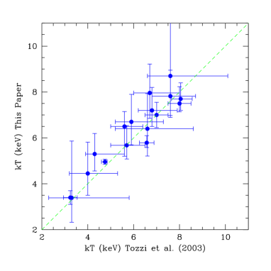
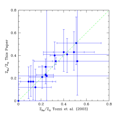
Figure 2: Comparison between the temperature (upper panel) and iron abundance (lower panel) values measured in Paper I, and those measured in this work after the most recent Chandra calibrations have been applied. Dashed lines show the locus of equal temperature and abundance values.

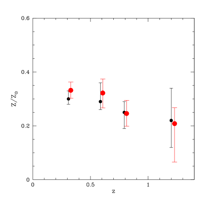
Figure 3: Average iron abundance in different redshift bins computed for the same sample of clusters analyzed in Paper I using updated calibrations (red circles), compared with the previous results (black circles). The plot shows that the new calibrations and data reduction have a negligible effect on our results. Only clusters with $kT>5$ keV are considered.

3.2 Single source analysis

This section presents the results of the spectral analysis of each of the 56 clusters of our sample. The results of the spectral fits, referring to the region of radius $R_{ext}$, defined in Sect. 2.1, are listed in Table 3. Histograms of the redshift and temperature distribution of the sample are shown in Figs. 4 and 5, respectively.

Table 3: Spectral fit results obtained with the tbabs(mekal) model.

Cluster	z	kT [keV]a	$Z/Z_{\odot}$ (And. & Gre.)b	$Z/Z_{\odot}$ (Aspl.)c	$N_{H}$ [cm-2]d	$\chi^{2}_{r}$ [d.o.f.] e	Null-Hyp. Prob.f
MS $1008.1-1224$	0.306	$5.8_{-0.2}^{+0.3}$	$0.30_{-0.06}^{+0.07}$	$0.47_{-0.10}^{+0.11}$	$7.26\times 10^{20}$	$1.23$ [228]	0.009
MS $2137.3-2353$	0.313	$4.96\pm 0.11$	$0.35\pm 0.03$	$0.56_{-0.05}^{+0.06}$	$3.55\times 10^{20}$	$1.23$ [289]	0.004
Abell 1995	0.319	$8.60\pm 0.32$	$0.40\pm 0.06$	$0.64_{-0.10}^{+0.10}$	$1.42\times 10^{20}$	$1.22$ [343]	0.003
MACS J$0308.9+2645$	0.324	$11.2\pm 0.7$	$0.37\pm 0.06$	$0.70_{-0.12}^{+0.10}$	$1.18\times 10^{21}$	$1.07$ [283]	0.194
ZwCl $1358.1+6245$	0.328	$6.70\pm 0.26$	$0.40\pm 0.06$	$0.64_{-0.10}^{+0.11}$	$1.92\times 10^{20}$	$1.23$ [282]	0.006
MACS J$0404.6+1109$	0.355	$6.9_{-0.8}^{+0.6}$	$0.16_{-0.11}^{+0.07}$	$0.22_{-0.20}^{+0.14}$	$1.43\times 10^{21}$	$1.01$ [165]	0.451
RX J$0027.6+2616$	0.367	$9.1_{-1.5}^{+2.6}$	$0.57_{-0.19}^{+0.27}$	$1.02_{-0.35}^{+0.34}$	$3.86\times 10^{20}$	$1.36$ [52]	0.042
MACS J$1720.2+3536$	0.391	$6.30\pm 0.33$	$0.50_{-0.06}^{+0.05}$	$0.83_{-011}^{+0.07}$	$3.40\times 10^{20}$	$0.74$ [189]	0.997
ZwCl $0024.0+1652$	0.395	$4.38\pm 0.27$	$0.75_{-0.18}^{+0.20}$	$1.22_{-0.29}^{+0.32}$	$4.20\times 10^{20}$	$1.02$ [128]	0.410
V $1416+4446$	0.400	$3.50\pm 0.18$	$0.88\pm 0.18$	$1.50_{-0.27}^{+0.35}$	$1.29\times 10^{20}$	$1.11$ [98]	0.219
MACS J$0159.8-0849$	0.405	$9.2_{-0.5}^{+0.6}$	$0.36\pm 0.05$	$0.59_{-0.09}^{+0.08}$	$2.08\times 10^{20}$	$1.13$ [208]	0.097
MACS J$2228.5+2036$	0.412	$7.9\pm 0.6$	$0.41_{-0.07}^{+0.06}$	$0.59_{-0.10}^{+0.09}$	$4.58\times 10^{20}$	$0.91$ [196]	0.801
MS $0302.7+1658$	0.424	$4.34_{-0.44}^{+0.56}$	$0.40_{-0.18}^{+0.21}$	$0.58_{-0.28}^{+0.34}$	$1.11\times 10^{21}$	$0.98$ [31]	0.490
MS $1621.5+2640$	0.426	$6.9_{-0.6}^{+0.7}$	$0.35_{-0.09}^{+0.08}$	$0.63\pm 0.14$	$3.58\times 10^{20}$	$0.90$ [157]	0.804
MACS J$0417.5-1154$	0.440	$11.3\pm 0.8$	$0.29_{-0.07}^{+0.06}$	$0.45_{-0.11}^{+0.10}$	$3.86\times 10^{20}$	$0.82$ [209]	0.971
MACS J$1206.2-0847$	0.440	$11.0_{-0.6}^{+0.7}$	$0.18_{-0.06}^{+0.05}$	$0.25_{-0.09}^{+0.10}$	$3.72\times 10^{20}$	$1.15$ [271]	0.045
RX J$1347.5-1145$	0.451	$14.0\pm 0.4$	$0.33\pm 0.04$	$0.55_{-0.06}^{+0.07}$	$4.92\times 10^{20}$	$1.20$ [436]	0.003
V $1701+6414$	0.453	$4.27_{-0.25}^{+0.26}$	$0.54_{-0.12}^{+0.13}$	$0.85_{-0.20}^{+0.22}$	$2.46\times 10^{20}$	$0.95$ [123]	0.649
CL $1641+4001$	0.464	$4.8\pm 0.6$	$0.48_{-0.16}^{+0.19}$	$0.79_{-0.24}^{+0.29}$	$1.10\times 10^{20}$	$0.98$ [53]	0.509
MACS J$1621.4+3810$	0.465	$6.5\pm 0.7$	$0.13\pm 0.08$	$0.19_{-0.16}^{+0.15}$	$1.09\times 10^{20}$	$1.46$ [67]	0.549
MACS J$1824.3+4309$	0.487	$7.2_{-1.3}^{+2.2}$	$0.38_{-0.25}^{+0.23}$	$0.55_{-0.33}^{+0.31}$	$4.46\times 10^{20}$	$1.03$ [33]	0.423
MACS J$1311.0-0311$	0.492	$8.0\pm 0.9$	$0.39\pm 0.09$	$0.60_{-0.19}^{+0.21}$	$1.87\times 10^{20}$	$0.97$ [87]	0.571
V $1525+0958$	0.516	$5.4_{-0.5}^{+0.4}$	$0.35\pm 0.10$	$0.54_{-0.20}^{+0.21}$	$2.91\times 10^{20}$	$1.06$ [107]	0.315
MS $0451.6-0305$	0.539	$8.2_{-0.3}^{+0.4}$	$0.34\pm 0.06$	$0.57\pm 0.10$	$4.97\times 10^{20}$	$1.24$ [279]	0.004
MS $0015.9+1609$	0.541	$9.3_{-0.3}^{+0.5}$	$0.33_{-0.05}^{+0.06}$	$0.53\pm 0.09$	$4.07\times 10^{20}$	$1.01$ [302]	0.460
MACS J$1149.5+2223$	0.544	$12.9_{-1.0}^{+1.2}$	$0.21_{-0.07}^{+0.06}$	$0.37_{-0.11}^{+0.10}$	$2.28\times 10^{20}$	$1.04$ [254]	0.317
MACS J$1423.8+2404$	0.545	$7.3_{-0.5}^{+0.6}$	$0.31_{-0.08}^{+0.06}$	$0.46_{-0.10}^{+0.13}$	$2.38\times 10^{20}$	$1.11$ [135]	0.174
MACS J$0717.5+3745$	0.548	$13.3\pm 0.7$	$0.18_{-0.04}^{+0.05}$	$0.29_{-0.07}^{+0.11}$	$7.04\times 10^{20}$	$1.14$ [404]	0.029
V $1121+2327$	0.562	$5.2\pm 0.5$	$0.27_{-0.08}^{+0.10}$	$0.43_{-0.07}^{+0.15}$	$1.32\times 10^{20}$	$0.99$ [102]	0.499
SC $1120-1202$	0.562	$5.7_{-0.8}^{+1.3}$	$0.23_{-0.17}^{+0.20}$	$0.33_{-0.21}^{+0.33}$	$5.19\times 10^{20}$	$1.13$ [45]	0.256
RX J$0848.7+4456$	0.570	$3.4\pm 0.30$	$0.51_{-0.19}^{+0.23}$	$0.79_{-0.30}^{+0.36}$	$2.63\times 10^{20}$	$1.33$ [46]	0.068
MACS J$2129.4-0741$	0.570	$8.7_{-0.8}^{+0.7}$	$0.51_{-0.11}^{+0.08}$	$0.82\pm 0.14$	$4.82\times 10^{20}$	$0.85$ [132]	0.890
MS $2053.7-0449$	0.583	$5.68_{-0.47}^{+0.57}$	$0.16_{-0.10}^{+0.11}$	$0.24_{-0.16}^{+0.18}$	$5.02\times 10^{20}$	$1.03$ [100]	0.402
MACS J$0647.7+7015$	0.584	$15.5_{-1.7}^{+2.3}$	$<0.10$	$<0.15$	$5.64\times 10^{20}$	$0.91$ [118]	0.737
RX J$0956.0+4107$	0.587	$7.4^{2.5}_{-1.45}$	$0.13_{-0.13}^{+0.28}$	$0.21_{-0.21}^{+0.45}$	$1.14\times 10^{20}$	$1.08$ [27]	0.353
CL $0542.8-4100$	0.634	$7.9_{-0.8}^{+1.1}$	$0.20_{-0.09}^{+0.12}$	$0.31_{-0.15}^{+0.19}$	$3.73\times 10^{20}$	$1.19$ [113]	0.081
RCS J$1419.2+5326$	0.640	$4.1_{-0.6}^{+0.7}$	$0.15_{-0.15}^{+0.21}$	$0.16_{-0.16}^{+0.31}$	$1.18\times 10^{20}$	$1.35$ [21]	0.131
MACS J$0744.9+3927$	0.686	$9.2\pm 0.6$	$0.28\pm 0.06$	$0.46_{-0.12}^{+0.10}$	$5.71\times 10^{20}$	$1.22$ [193]	0.021
RX J$1221.4+4918$	0.700	$8.4_{-0.8}^{+0.9}$	$0.29_{-0.12}^{+0.13}$	$0.48_{-0.19}^{+0.21}$	$1.47\times 10^{20}$	$0.99$ [141]	0.534
RX J$1113.1-2615$	0.730	$5.7_{-0.6}^{+0.9}$	$0.43_{-0.17}^{+0.20}$	$0.68_{-0.27}^{+0.30}$	$5.50\times 10^{20}$	$0.69$ [59]	0.966
RX J$2302.8+0844$	0.734	$8.0_{-1.1}^{+1.3}$	$0.12_{-0.12}^{+0.16}$	$0.19_{-0.19}^{0.26}$	$4.85\times 10^{20}$	$0.85$ [81]	0.833
MS $1137.5+6624$	0.782	$6.8\pm 0.5$	$0.26\pm 0.11$	$0.43_{-0.17}^{+0.18}$	$1.21\times 10^{20}$	$1.09$ [151]	0.204
RX J$1317.4+2911$	0.805	$4.5_{-1.0}^{+1.4}$	$0.35_{-0.30}^{+0.46}$	$0.49_{-0.46}^{+0.67}$	$1.10\times 10^{20}$	$0.71$ [14]	0.768
RX J$1350.0+6007$	0.810	$4.4_{-0.6}^{+0.7}$	$0.56_{-0.18}^{+0.27}$	$0.96_{-0.33}^{+0.35}$	$1.80\times 10^{20}$	$1.26$ [51]	0.103
RX J$1716.4+6708$	0.813	$6.9_{-0.7}^{+0.8}$	$0.49_{-0.16}^{+0.18}$	$0.79_{-0.26}^{+0.29}$	$3.72\times 10^{20}$	$0.77$ [76]	0.934
RX J$0152.7-1357$ S	0.828	$8.7_{-1.8}^{+2.4}$	$<0.22$	$<0.37$	$1.54\times 10^{20}$	$1.06$ [32]	0.376
MS $1054.4-0321$	0.832	$7.5_{-0.4}^{+0.7}$	$0.23_{-0.08}^{+0.07}$	$0.38_{-0.12}^{+0.12}$	$3.61\times 10^{20}$	$1.15$ [238]	0.056
RX J$0152.7-1357$ N	0.835	$6.7_{-1.0}^{+1.2}$	$0.17_{-0.16}^{+0.19}$	$0.25_{-0.25}^{+0.30}$	$1.54\times 10^{20}$	$0.87$ [45]	0.715
1WGA J$1226.9+3332$	0.890	$12.9_{-1.2}^{1.4}$	$0.02_{-0.02}^{+0.12}$	$<0.21$	$1.38\times 10^{20}$	$1.06$ [97]	0.335
CL $1415.1+3612$	1.030	$7.0_{-0.7}^{+0.8}$	$0.24_{-0.13}^{+0.15}$	$0.40_{-0.21}^{+0.23}$	$1.09\times 10^{20}$	$0.79$ [63]	0.891
RDCS J$0910+5422$	1.106	$6.4_{-1.2}^{+1.5}$	$<0.14$	$<0.21$	$2.10\times 10^{20}$	$0.94$ [28]	0.559
RX J$1053.7+5735$ E	1.134	$3.4_{-0.4}^{+0.5}$	$0.51_{-0.15}^{+0.14}$	$0.58_{-0.22}^{+0.75}$	$5.7\times 10^{19}$	$1.11$ [29]	0.317
RX J$1053.7+5735$ W	1.134	$7.2_{-0.9}^{+1.2}$	$0.32_{-0.15}^{+0.14}$	$0.51_{-0.24}^{+0.23}$	$5.7\times 10^{19}$	$0.55$ [31]	0.981
RDCS J$1252-2927$	1.235	$7.2_{-0.6}^{+0.4}$	$0.35_{-0.09}^{+0.06}$	$0.58_{-0.15}^{+0.11}$	$5.95\times 10^{20}$	$1.01$ [55]	0.454
RDCS J$0849+4452$	1.261	$6.2_{-0.9}^{+1.0}$	$0.16_{-0.14}^{+0.13}$	$0.21_{-0.19}^{+0.27}$	$2.63\times 10^{20}$	$0.51$ [24]	0.977
RDCS J$0848+4453$	1.273	$3.4_{-1.1}^{+2.5}$	$0.22_{-0.22}^{+1.33}$	$0.22_{-0.22}^{+1.38}$	$2.63\times 10^{20}$	$1.04$ [11]	0.411

• ^a temperature; ^b iron abundance in solar units by Anders & Grevesse (1989) and ^c by Asplund et al. (2005); ^d local column density, always fixed to the Galactic value by Dickey & Lockman (1990); ^e reduced chi-square and degrees of freedom obtained after binning the spectra to 20 counts per bin; ^f null-hypothesis probability. Errors refer to the $1\sigma$ confidence level.

Figure 4: Histogram of the redshift distribution of the sample. The solid line refers to the whole sample, while the dotted line displays only clusters with $kT\leq 5$ keV (see Table 3). The vertical dotted lines indicate the five redshift intervals selected for the combined spectral analysis, as described in the text.

Figure 5: Histogram of the temperature distribution of the sample. The vertical dotted line separates the moderate temperature ($kT<5$ keV) clusters from the high temperature ($kT>5$ keV) clusters.

The redshift distribution is peaked around $z\simeq 0.5$, while at $z>1$ we have only 7 objects (we recall that we consider the two clumps of RX J1053 separately, see Hashimoto et al. 2004). In order to investigate the properties of the sample as a function of redshift, we divide the clusters in 5 redshift intervals (10 objects with $0.3<z<0.4$; 12 objects with $0.4<z<0.5$; 15 objects with $0.5<z<0.65$; 12 objects with $0.65<z<1.0$, and 7 objects with $1.0<z<1.3$). These intervals (Fig. 4) are defined in order to have a comparable number of objects in a reasonably narrow redshift range.

As shown in the temperature distribution (Fig. 5), we sampled mostly hot clusters ($kT>5$ keV), while only 12 are in the medium temperature range ($3<kT<5$ keV). We would like to point out here that we derived a single spectral temperature for the region within $R_{ext}$. In principle, the spectral temperature can be significantly different from the emission-weighted and gas-mass-weighted temperature, in the presence of a thermally complex ICM (e.g. Mazzotta et al. 2004). In a few cases, the effect of the temperature gradient is strong enough to make the single-temperature fit unacceptable. To evaluate the goodness of each fit, we computed the $\chi^{2}$ of each best-fit model after binning the spectrum to 20 counts per bin. We find that most of our spectra are well-fitted by a single-temperature mekal model (see 7th column in Table 3). However, when the number of the net detected counts becomes larger than $\sim 10^{4}$, the quality of the fits drops dramatically for about half of the clusters (see Fig. 6). If we consider a 1% null-hypothesis probability as the threshold for an acceptable fit, then we must reject the single-temperature model within $R_{ext}$ for 5 clusters in our sample (namely MS 2137, A 1995, ZW 1358, RX J1347, and MS 0451). Note that we can also fit clusters with very disturbed morphology and high S/N (e.g. MACS J0717) with a single-temperature model, due to the very high temperatures involved, which provide composite spectra with much less features than spectra with low-temperature components. Indeed, the single-temperature model fails mostly when a strong cool-core with temperatures lower than 3 keV is present (e.g. Mazzotta et al. 2004), while it is still acceptable if the temperature range is well above this threshold.

Figure 6: Null-hypothesis probability for the single-temperature best fits as a function of net detected counts for the whole sample.

Since we are focusing here on metallicity, we made a closer investigation of the best-fit $Z_{Fe}$ values for the clusters with the lowest null-hypothesis probability. Since these clusters are also the ones with the highest S/N, we were able to perform a spatially resolved spectral analysis for about four concentric annuli. We find that the best-fit $Z_{Fe}$ value measured with a single temperature mekal model within $R_{ext}$, is representative of the inner 400 kpc and is not dominated by the central bin. This result, implying that the presence of temperature gradient does not dramatically affect the measurements of iron abundance, is reinforced by the spectral simulations described in the Appendix. Therefore we used the single-temperature best-fit values for all the clusters in our sample. The attempt to model the evolution of $Z_{Fe}$ separately in the inner 100 kpc and the outer regions is deferred to a future paper.

Finally, we show in Fig. 7 the distribution of temperatures in our sample as a function of redshifts (error bars are at the $1\sigma$ confidence level). The Spearman test shows no correlation between temperature and redshift (Spearman’s rank coefficient of $r_{s}=-0.095$ for 54 degrees of freedom, probability of null correlation $p=0.48$). Fig. 7 shows that the range of temperatures in each redshift bin is about $6-7$ keV. Therefore, we are sampling a population of medium-hot clusters uniformly with redshift, with the hottest clusters preferentially in the redshift bin $0.4<z<0.6$.

Figure 7: Temperature plotted vs redshift for the whole sample. Shaded areas show the rms dispersion around the weighted mean.

The relations between temperature and iron abundance at different redshifts are shown in Fig. 8. For three clusters we can only derive upper limits on the iron abundance of the ICM, two of them at $z<0.8$. For five clusters we measure positive iron abundances, which are still consistent with no detection at the $1\sigma$ c.l.. Overall, we detect the presence of the iron line in the large majority of the clusters, and measure the iron abundance with a typical error of 30% at the $1\sigma$ c.l. for $z<0.6$, and 50% or larger at $z>0.6$.

Figure 8: Iron abundance-temperature plots for the whole sample. The four panels show each redshift bin separately (last two bins in the fourth panel). The dashed line represents the best-fit metallicity-temperature relation ($Z/Z_{\odot}\simeq 0.88\,T^{-0.47}$) referring to the whole sample. Error bars refer to $1\sigma$ confidence level.

3.3 The iron abundance-temperature correlation

Our analysis (Fig. 9) suggests higher iron abundances at lower temperatures in all the redshift bins. This trend is somewhat blurred by the large scatter. We find a more than $2\sigma$ negative correlation for the whole sample, with a Spearman’s rank coefficient of $r_{s}=-0.31$ for 54 degrees of freedom (probability of no correlation $p=0.018$). The correlation is more evident when we compute the weighted average of the metallicity in six temperature intervals (see Table 4), as shown by the shaded areas in Fig. 9. The weighted mean is computed as $T_{wa}=\,\Sigma T_{i}w_{i}$ in each temperature bin, where $w_{i}=1/\sigma_{i}^{2}/\Sigma(1/\sigma_{i}^{2})$, and $\sigma_{i}$ is the $1\sigma$ error on the single measurement. We find that in each bin the scatter of the best-fit values around the mean is comparable to the statistical errors on the single measurements (reduced $\chi_{\nu}^{2}\simeq 1$ assuming a constant $Z_{Fe}$ in the bin), with the exception of the third and sixth bins, where the intrinsic scatter is larger ($\chi_{\nu}^{2}\simeq 3$).

Figure 9: Scatter plot of best-fit iron abundance values (without error bars) versus temperature for the whole sample. The dashed line represents the best-fit metallicity-temperature relation ($Z/Z_{\odot}\simeq 0.88\,T^{-0.47}$). Shaded areas show the weighted mean (blue) and average iron abundance with rms dispersion (cyan) in 6 temperature bins (see Table 4).

Table 4: Average iron abundance calculated in different temperature bins.

$kT$ [keV]a	$Z/Z_{\odot}\mathrm{{}^{b}}$	$\Delta Z/Z_{\odot}\mathrm{{}^{c}}$
	(weighted mean)	(rms)
$3.9$ [10]	$0.542\pm 0.060$	$0.23$
$5.4$ [8]	$0.329\pm 0.024$	$0.10$
$6.7$ [11]	$0.322\pm 0.027$	$0.17$
$7.5$ [10]	$0.317\pm 0.030$	$0.11$
$8.8$ [9]	$0.350\pm 0.024$	$0.16$
$12.7$ [8]	$0.244\pm 0.021$	$0.14$

• ^a average temperature in each bin (the number of clusters in each bin is shown in parenthesis); ^b weighted mean of the iron abundance; ^c rms dispersion.

This trend is similar to what is found in the ASCA data of nearby clusters by Baumgartner et al. 2005 (see also Arnaud et al. 1992; Mushotzky & Loewenstein 1997; Finoguenov et al. 2001). In their paper, the average iron abundance for $kT>5$ keV is constant and equal to $Z\simeq 0.3\,Z_{\odot}$, while it rises to very high values (well above $0.4\,Z_{\odot}$) in the temperature range $2-3$ keV, and drops below $0.3\,Z_{\odot}$ for $kT<2$ keV. It is worth noting, however, that this behavior is different from that of Ni and $\alpha$-elements. Here, we confirm that in our high-redshift sample the average measured iron abundance rises below 5 keV. A simple power law fit of the form

$$Z(T)=Z_{Fe}(0)\,T^{-\alpha_{T}}$$ (3)

to our data gives $Z_{Fe}(0)=0.88^{+0.5}_{-0.2}\,Z_{\odot}$ and $\alpha_{T}=-0.47^{+0.1}_{-0.2}$ with $\chi_{\nu}^{2}\simeq 1.8$ for 5 degrees of freedom (see the confidence contours in the slope-normalization plane in Fig. 10). This trend is consistent with what is found from ASCA data of a local sample of clusters for $kT>3$ keV (see Baumgartner et al. 2005; Horner 2005). Interestingly, a similar correlation between temperature and metallicity is observed when a spatially-resolved analysis of the ICM can be performed in a single object, as in the case of the core of the Perseus cluster (see Sanders et al. 2004). However a physical explanation for this behaviour is still missing.

Figure 10: Best-fit confidence contour plot for the $Z-T$ relation modelled with a power law of the form $Z(T)=Z_{Fe}(0)\,T^{-\alpha_{T}}$. Inner contours display the 1, 2, and $3\sigma$ c.l. using errors on the weighted mean, while outer thick contours are obtained using the rms dispersion.

We recall that the measure of the iron abundance in local clusters is based on both the K-shell and the L-shell complex, at $6.7-6.9$ keV and between 1 and 2 keV, respectively. It has been pointed out that a diagnostic based mostly on the L-shell, as in the case of spectra with a significant low temperature component, is more uncertain (Renzini 1997). In our high redshift sample, we expect to be sensitive only to the iron K-shell complex. Indeed, when we fit the spectra cutting energies below 2 keV rest-frame, we find that the best-fit metallicities are consistent with those found within the $0.6-8$ keV range (observed frame) used throughout the paper, as shown in Fig. 11. We notice that when the low energy range is removed, errors on the temperatures become larger, with a clear tendency to higher values. This trend is expected since higher temperature spectral shapes can be accommodated more easily than lower ones. On the other hand, iron abundances hardly change, except for the two most iron-rich clusters, ZW 0024 and V 1416. This may indicate that in these two objects the high iron abundance could be associated with a low temperature component. However, in these cases a separate analysis in two annuli is possible and we do not find a clear enhancement of the iron abundance in the inner regions.

The observed trend between $Z_{Fe}$ and $T$ is still a matter of debate. It may be linked to the observed decrease in the star formation efficiency with increasing cluster mass as reported in Lin et al. (2003). The modelization of this trend goes beyond the scope of this paper.

Figure 11: Best-fit temperatures (upper panel) and iron abundances (lower panel) obtained using the $1.5-8$ keV energy range compared to the values obtained from the $0.6-8$ keV (this paper). Dashed lines show the locus of equal temperatures and abundances. Only clusters with more than 2000 net counts (see Table 1) are considered here.

3.4 The evolution of the iron abundance via combined spectral analysis

In Fig. 12 we show the iron abundance best-fit values for all the sources in the sample. When focusing on the highest redshift bin, it is worth noticing that at $z>1$ we find clear detections of the Fe K line in the spectra of CL J1415 ($z=1.030$, $Z_{Fe}>0$ at the 90% c.l.), of RDCS J1252 ($z=1.235$, $Z_{Fe}>0.2\,Z_{\odot}$ at the 90% c.l.), and of the two clumps of RX J1053 ($z=1.134$, $Z_{Fe}>0.1\,Z_{\odot}$ at the 90% c.l.). In the spectra of the four other clusters, we do not have separate detections of the iron line, but all measurements are consistent within $1\sigma$ with $Z_{Fe}\simeq 0.3\,Z_{\odot}$. Therefore, at present, we have a much better estimate of the metal content of clusters at $z\simeq 1$ than in Paper I, where the iron line at $z>1$ was only firmly detected in the two clumps of RX J1053.

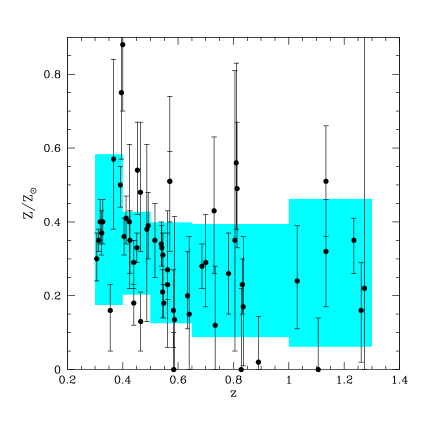
Figure 12: Iron abundance plotted versus redshift for the 56 clusters of the sample. Shaded areas show the rms dispersion around the weighted mean of the iron abundance in the 5 redshift bins defined in the text. Error bars refer to a $1\sigma$ confidence level.

We find a $\sim 3\sigma$ negative correlation between iron abundance and redshift, with a Spearman’s rank coefficient of $r_{s}=-0.40$ for 54 degrees of freedom (probability of a null correlation $p=0.0023$). This correlation is stronger than the weak hint (less than a $2\sigma$ c.l.) of anticorrelation found in Paper I. We verified that, if we calculate the Spearman’s rank coefficient only for the 19 clusters analyzed in Paper I, using the newly revised temperature and abundances (consistent with the old ones as shown in Fig. 2), we again obtain very weak correlation ($r_{s}=-0.25$ for 17 degrees of freedom, probability of no correlation $p=0.30$), which is therefore consistent with the results reported in Paper I. This confirms that our new results should not be ascribed to updated calibrations, but rather to the larger size of the sample, particularly at $z<0.5$.

The decrease in $Z_{Fe}$ with redshift becomes more evident by computing the average iron abundance as determined by a combined spectral fit in a given redshift bin. This technique is similar to the stacking analysis often performed in optical spectroscopy, where spectra from a homogeneous class of sources are averaged together to boost the S/N, thus allowing the study of otherwise undetected features. In our case, different X-ray spectra cannot be stacked due to their different shape (different temperatures). Therefore, a simultaneous spectral fit is performed leaving temperature and normalization free to vary for each object, and using a unique metallicity value for all the clusters in the subsample.

We note that the scatter of the best-fit values around the mean in each redshift bin is, in some cases, larger than the typical statistical errors on single measurements. This is expected on the basis of the $Z-T$ correlation, as found in Sect. 3.3. The reduced $\chi^{2}$ obtained by assuming that measurements are scattered around the weighted average is between 2 and 3 in the first two bins, implying the presence of intrinsic scatter comparable to the typical statistical error, while it is $\sim 1$ above $z\simeq 0.5$, since here the typical statistical error is larger than the intrinsic scatter component. By assuming a unique value of $Z_{Fe}$ in the combined fit, however, we intend to provide an average value of the metallicity over large cluster volumes as a function of redshift.

A plot of the combined iron abundance measured in each redshift bin is shown in Fig. 13. To verify the robustness of our results, we computed the weighted average from the single source fits in each redshift bin. The best-fit values resulting from the combined fits are always consistent with the weighted means (listed in Table 5) within $1\sigma$, except for the bin at $z\sim 0.6$, which is lower. We also checked that, if the two clusters with the highest $Z_{Fe}$ (i.e. ZW 0024 and V1416, see Sect. 3.3) are removed from the fit, the average $Z_{Fe}$ value in the first redshift bin is only slightly changed (at the level of $\sim 3\%$).

Table 5: Average iron abundance in different redshift bins resulting from combined fit and weighted mean.

$\langle z\rangle\mathrm{{}^{a}}$	$Z/Z_{\odot}\mathrm{{}^{b}}$	$Z/Z_{\odot}\mathrm{{}^{c}}$	$\Delta Z/Z_{\odot}\mathrm{{}^{d}}$
	(combined fit)	(weighted mean)	(rms)
0.206 [9]	$0.427^{+0.003}_{-0.011}$	$0.416\pm 0.009$	$0.08$
0.350 [10]	$0.387_{-0.012}^{+0.013}$	$0.379\pm 0.019$	$0.20$
0.447 [12]	$0.330^{+0.017}_{-0.012}$	$0.318\pm 0.020$	$0.11$
0.572 [15]	$0.306^{+0.017}_{-0.033}$	$0.260\pm 0.020$	$0.13$
0.787 [12]	$0.244\pm 0.025$	$0.251\pm 0.035$	$0.15$
1.167 [7]	$0.265_{-0.04}^{+0.05}$	$0.28\pm 0.048$	$0.15$

• ^a average redshift of each bin (the number of clusters in each bin is shown in parenthesis); ^b iron abundance from combined fit with $1\sigma$ errors; ^c iron abundance from weighted mean; ^d rms dispersion.

Figure 13: Mean iron abundance from combined fits within five redshift bins defined in the text (red circles) compared with the weighted average of single-source measurements in the same bins (black squares). The triangles at $z\simeq 0.2$ are based on the low-z sample described in Sect. 3.5. Error bars refer to the $1\sigma$ confidence level. Shaded areas show the rms dispersion. The dashed line indicates the best fit over the 6 redshift bins for a simple power law of the form $\langle Z_{Fe}\rangle=Z_{Fe}(0)\,(1+z)^{-\alpha_{z}}$ with $\alpha_{z}\simeq 1.25$.

From a visual inspection of Fig. 13, we notice a continuous trend of decreasing iron abundance from $z\simeq 0.3$ to $z\simeq 1.2$. While a constant value $\langle Z_{Fe}\rangle\simeq 0.25\,Z_{\odot}$ is a good fit at $z>0.5$, the iron abundance is significantly higher at $z<0.5$, the redshift range over which the statistics of our sample increased most with respect to Paper I. In addition, we now have a firm measurement of the average iron abundance at redshift $z\simeq 0.8$ and $z\simeq 1.2$, reinforcing the results of Paper I; in particular, the iron abundance in the most distant clusters is still consistent with the value $Z_{Fe}=0.3\,Z_{\odot}$ within $1\sigma$.

Given the negative correlation between iron abundance and temperature found in our sample (see Sect. 3.3), we first verified whether the evolution with redshift is due to the presence of low-temperature clusters in the low redshift bins. By excluding clusters with $kT<5$ keV from the plot, the same results are obtained, as expected from the lack of correlation betwen the average temperature and redshift found in Sect. 3.2.

We also note that this trend points towards $\langle Z_{Fe}\rangle\sim 0.5\,Z_{\odot}$ at low-z, which is higher than the often-reported value $Z_{Fe}\simeq 0.3\,Z_{\odot}$. The reason is that we are measuring $Z_{Fe}$ in the inner regions of clusters, where it reaches values significantly higher than $0.3\,Z_{\odot}$, particularly in cool-core clusters (see Vikhlinin et al. 2005), which constitute about 2/3 of the local population. In order to show that the average iron abundance in low-z clusters, when analyzed with our procedure, confirm the trend seen in the high-z sample, we add a point at $\langle z\rangle\simeq 0.2$ including 9 clusters, as described in detail in Sect. 3.5.

A fit with a constant iron abundance value over the entire redshift range is unacceptable. If we model the evolution (including the additional low-z point, using the values from the combined fits) with a simple power law as

$$\langle Z_{Fe}\rangle\simeq Z_{Fe}(0)\,(1+z)^{-\alpha_{z}}\,,$$ (4)

the best-fit values obtained are $Z_{Fe}(0)=0.54\pm 0.04\,Z_{\odot}$ and $\alpha_{z}=1.25\pm 0.15$ ($\chi_{\nu}^{2}=0.9$), implying a decrease by a factor of $\sim 2$ between $z=0.3$ and $1.2$. The evolution ($\alpha_{z}<0$) is significant only at $1\sigma$ level when the rms dispersion is used instead of the errors on the combined fits (see confidence contours in Fig. 14). However, the rms dispersion is greatly overestimating the uncertainties on the average values. Consistent best-fit results are obtained if the lowest redshift point is excluded from the fit or if weighted mean values are used.

Figure 14: Best-fit confidence contours plot for the metallicity as a function of redshift (including the additional low-z point) modelled with a power law of the form $Z(z)=Z_{Fe}(0)\,(1+z)^{-\alpha_{z}}$. Thick inner contours display the 1, 2, and $3\sigma$ c.l. using the results of the combined fits, while thin outer contours are obtained using the rms dispersion.

3.5 The “local” iron abundance of the ICM

An important issue to address is how our findings at $z\ga 0.3$ compare with the local iron abundance, which is traditionally quoted to be $Z_{Fe}\simeq 0.3\,Z_{\odot}$ (Renzini 1997) in the units following Anders & Grevesse (1989). The spatially-resolved spectroscopy of local clusters obtained with the Chandra and XMM-Newton satellites shows a complex distribution of the metals within the inner regions. The large differences in iron abundances and gradients from cluster to cluster lessens the meaning of the adoption of a single canonical value for the average iron content of the ICM in the local Universe. The value $Z_{Fe}\simeq 0.3\,Z_{\odot}$ is typically observed only in non cool-core clusters or in the outer regions ($>100$ kpc) of cool-core clusters (see Tamura et al. 2004 for XMM-Newton and Vikhlinin et al. 2005 for Chandra data). The central peak of iron abundance reaches values of $Z_{Fe}\simeq(0.6-0.8)\,Z_{\odot}$ in the cores of cool-core clusters, which have a typical size of 100 kpc (see De Grandi et al. 2004; Vikhlinin et al. 2005), whereas $Z_{Fe}$ decreases to $\simeq 0.3\,Z_{\odot}$ in the outer regions. On the other hand, the iron abundance appears to be constant, $Z_{Fe}\simeq 0.2-0.3\,Z_{\odot}$, in non cool-core clusters. As a result, particular care should be used when comparing our measurements with the local values of $Z_{Fe}$ from the literature.

Since the extrapolation of the average $Z_{Fe}$ at low-z points towards $Z_{Fe}(0)\simeq 0.5\,Z_{\odot}$, we need to explain the apparent discrepancy with the oft-quoted canonical value $\langle Z_{Fe}\rangle\simeq 0.3\,Z_{\odot}$. As mentioned in Sect. 3.4, the discrepancy is due to the fact that our average values are computed within $r\simeq 0.15\,R_{vir}$, where the iron abundance is boosted by the presence of metallicity peaks often associated to cool cores. The regions chosen for our spectral analysis, are larger than the typical size of the cool cores, but smaller than the typical regions adopted in studies of local samples.

This can be proved by analyzing the inner regions ($r<0.15\,R_{vir}$) of a sample of clusters at $z<0.3$. We selected a small subsample of 9 clusters at redshift $0.1<z<0.3$, including 7 cool-core and 2 non cool-core clusters, a mix that is representative of the low-z population. These clusters, listed in Table 6, are presently being analyzed for a separate project aimed at obtaining spatially-resolved spectroscopy (Baldi et al., in preparation). Here we analyze a region within $r=0.15\,R_{vir}$ in order to probe the same regions probed at high redshift. We used this small control sample to add a low-redshift point in our Fig. 13, which extends the $Z_{Fe}$ evolutionary trend.

Table 6: Spectral fit results for the low-z sample with the tbabs(mekal) model.

Cluster	z	kT [keV]a	$Z/Z_{\odot}\mathrm{{}^{b}}$	$N_{H}$ [cm-2]c	$\chi^{2}_{r}$ [d.o.f.]d	Null Hyp. Prob.e
Abell~1413	0.143	$7.1\pm 0.1$	$0.39\pm 0.02$	$2.18\times 10^{20}$	1.55 [477]	$10^{-13}$
Abell~907	0.153	$5.2\pm 0.1$	$0.53\pm 0.03$	$5.36\times 10^{20}$	1.37 [431]	$10^{-7}$
Abell~2104	0.155	$13.9\pm 0.5$	$0.53_{-0.07}^{+0.04}$	$8.69\times 10^{20}$	1.35 [423]	$10^{-6}$
Abell~2218	0.176	$7.9\pm 0.3$	$0.26\pm 0.03$	$3.26\times 10^{20}$	1.09 [347]	0.111
Abell~963	0.206	$7.0\pm 0.2$	$0.43\pm 0.03$	$1.40\times 10^{20}$	1.09 [341]	0.113
Abell~2261	0.224	$7.5_{-0.2}^{+0.4}$	$0.51_{-0.05}^{+0.03}$	$3.28\times 10^{20}$	1.07 [329]	0.169
Abell~2390	0.228	$9.1\pm 0.1$	$0.40_{-0.02}^{+0.03}$	$6.81\times 10^{20}$	1.50 [479]	$10^{-12}$
Abell~1835	0.253	$7.2\pm 0.2$	$0.41_{-0.04}^{+0.03}$	$2.32\times 10^{20}$	0.99 [291]	0.527
ZwCl~$1021.0+0426$	0.291	$6.2\pm 0.1$	$0.39_{-0.03}^{+0.03}$	$3.02\times 10^{20}$	1.51 [396]	$10^{-10}$

• ^a temperature; ^b iron abundance in solar units by Anders & Grevesse (1989); ^c local column density, always fixed to the Galactic value by Dickey & Lockman (1990); ^d reduced chi-square and degrees of freedom obtained after binning the spectra to 20 counts per bin; ^e null-hypothesis probability. Errors refer to the $1\sigma$ confidence level.

4 Discussion

The main result of this work is that the cosmic average of $Z_{Fe}$ in the central regions ($R<0.3\,R_{vir}$) of clusters significantly decreases with redshift out to $z\simeq 0.5$, remaining constant out to $z\simeq 1.3$ at the level of $Z_{Fe}\simeq 0.25$. Given the complex thermal and chemical structures observed in bright local clusters, a main concern is whether our analysis might be affected by evolution in the occurrence of temperature/metallicity gradients in the cluster population. The assumption of a single-temperature mekal model for the inner $0.3\,R_{vir}$ may well be too simplistic, and it may introduce systematic biases in the recovered $Z_{Fe}$ values. In order to clarify this issue, we investigate possible biases in our fitting procedure in the Appendix using a large set of simulated spectra in the typical S/N regime of our high-z clusters. We find that different S/N values do not introduce any significant bias. In particular, spectra with lower S/N (occurring mostly at high-redshift) tend to give slightly higher $Z_{Fe}$ compared to the input values, therefore opposite to the observed trend (see Fig. A.1).

In the Appendix we also investigate the cases of a two-temperature ICM with a single $Z_{Fe}$ and of a two-temperature ICM with higher $Z_{Fe}$ associated with the colder component, analyzed with a single-temperature mekal model. Here the key parameter is the ratio of the emission measure of the two components. This quantity is difficult to model, so that here we assume a few representative values ranging from 0.3 to 0.75.

In both cases we measured slightly higher temperatures at higher redshifts, due to the fact that for high-redshift clusters, the signature of the cold component is partially redshifted below the adopted energy range ($E>0.6$ keV). We also find a mild trend toward lower $Z_{Fe}$ at $z\sim 1$ compared to $z\sim 0.6$. This effect is limited to be $\leq 30$%, and therefore it cannot fully explain the observed decrease even under the extreme assumption that all the clusters in the sample had steep temperature gradients with a central abundance peak. To sum up, these simulations show that the presence of temperature and abundance gradients, if their occurrence is constant through the population of clusters at different redshifts, does not introduce significant bias into our measure of the evolution of $Z_{Fe}$.

Furthermore, we investigate whether the evolution of $Z_{Fe}$ could be due to an evolving fraction of clusters with cool cores, which are known to be associated with iron-rich cores (see De Grandi et al. 2004) and which amount to more than 2/3 of the local clusters (see Bauer et al. 2005). For example, the evolution of the mass in iron in the central peak, which is about $20-30$% of the total, may be associated with the star formation product of the central galaxy alone (see De Grandi et al. 2004).

In order to use a simple characterization of cool-core clusters in our high-z sample, we computed the ratio of the fluxes emitted within 50 and 500 kpc ($C=f(r<50\,kpc)/f(r<500\,kpc$) computed as the integral of the surface brightness in the $0.5-5$ keV band (observer frame). This quantity ranges between 0 and 1 and it represents the relative weight of the central surface brightness. Higher values of $C$ are expected if a cool core is present. If the decrease in $Z_{Fe}$ with redshift is associated to a decrease in the number of cool-core clusters for higher $z$, we would expect to observe a positive correlation between $Z_{Fe}$ and $C$ and a negative correlation between $C$ and redshift. In Fig. 15 we plot $Z_{Fe}$ as a function of $C$ for our sample. We find that in our sample there is no correlation between metallicity and $C$ with a Spearman’s coefficient of $r_{s}=0.02$ (significance of $\sim 0.2\sigma$) nor one between $C$ and redshift ($r_{s}=-0.11$, a level of confidence of $0.8\sigma$).

The absence of strong correlations between $C$ and iron abundance or between $C$ and redshift suggests that the mix of cool cores and non cool cores over the redshift range studied in the present work cannot justify the observed evolution in the iron abundance. We caution, however, that a possible evolution of the occurrence of cool-core clusters at high redshift may still partially contribute to the observed evolution of $Z_{Fe}$. In other words, whether the observed evolution of $Z_{Fe}$ is contributed entirely by the evolution of the mass of iron or is partially due to a redistribution of iron in the central regions of clusters is an open issue to be addressed with a proper and careful investigation of the surface brightness of the high-z sample.

Figure 15: Iron abundance plotted versus $C=f(r<50\,kpc)/f(r<500\,kpc)$. Clusters within different redshift bins are coded with different symbols.

A final check is provided by the scatter plot of $Z_{Fe}$ versus $R_{ext}/R_{vir}$, shown in Fig. 16. We do not detect any dependence of $Z_{Fe}$ on the extraction radius adopted for the spectral analysis. In particular, we find that clusters with smaller extraction radii do not show higher $Z_{Fe}$ values.

Figure 16: Iron abundance plotted versus the ratio $R_{ext}/R_{vir}$. Shaded areas show the rms dispersion around the average iron abundance in four bins.

Together with the previous discussion of possible selection biases of our sample, all these tests concur to indicate that the observed evolution of the iron abundance is a genuine signature of some physical processes associated with the production and release of iron into the ICM.

This finding may be directly interpreted in terms of the cosmic star formation history (see Ettori 2005) for high assumed values of the time delay of SNe Ia (see Dahlen et al. 2004), which are expected to be the main contributors of iron. Other works (e.g. Mannucci et al. 2006) argue that the data on (i) the evolution of the SN Ia rate with redshift, (ii) the enhancement of the SN Ia rate in radio-loud early type galaxies, and (iii) the dependence of the SN Ia rate on the colours of the parent galaxies suggest the existence of two populations of progenitors for SN Ia. One population is expected to explode soon after the stellar birth on a time scale of $10^{8}$ years and can significantly pollute the ICM with iron at high redshift. The second population contributes to late enrichment with an exponential decay time of $\sim 3$ Gyrs. Following the argument described in Ettori (2005), we note that the rates adopted by Mannucci et al. (2005) predict a flatter distribution of the iron abundance as function of redshift than the rates tabulated in Dahlen et al. (2004), with a milder negative evolution still partially consistent with our measurements. Using detailed chemical evolution models, Loewenstein (2006) has recently interpreted the significant enrichment of the ICM at $z\simeq 1$ as direct evidence of prompt star formation in spheroids with a top-heavy IMF. Moreover, these models generally predict a significant increase in the iron abundance between $z=0$ and $z=1$, in qualitative agreement with our results.

Alternatively, the evolution in $Z_{Fe}$ occurring in the 5 Gyr spanned by our sample may be ascribed to some dynamical processes that transfer the metal-enriched gas from the intergalactic medium of the cluster galaxies to the hot phase of the ICM. Mechanisms such as ram pressure (Domainko et al. 2004; Cora 2006) or tidal stripping (e.g. Murante et al. 2004) are currently being investigated with numerical simulations (see also Valdarnini 2003; Tornatore et al. 2004). The same mechanisms are often invoked to explain the morphological evolution of the cluster galaxies’ population.

5 Conclusions

We have presented the spectral analysis of 56 clusters of galaxies at intermediate-to-high redshifts observed by Chandra and XMM-Newton. This work improves our first analysis aimed at tracing the evolution of the iron content of the ICM out to $z\ga 1$ (Paper I), by substantially extending the sample. The main results of our work can be summarized as follows:

• We determine the average ICM iron abundance with a $\sim 20$% uncertainty at $z>1$ ($Z_{Fe}=0.27\pm 0.05\,Z_{\odot}$), thus confirming the presence of a significant amount of iron in high-z clusters. $Z_{Fe}$ is constant above $z\simeq 0.5$, the largest variations being measured at lower redshifts.

• We find a significantly higher average iron abundance in clusters with $kT<5$ keV, in agreement with trends measured in local samples. For $kT>3$ keV, $Z_{Fe}$ scales with temperature as $Z_{Fe}(T)\simeq 0.88\,T^{-0.47}$.

• We find significant evidence of a decrease in $Z_{Fe}$ as a function of redshift, which can be parametrized by a power law $\langle Z_{Fe}\rangle\simeq Z_{Fe}(0)\,(1+z)^{-\alpha_{z}}$, with $Z_{Fe}(0)\simeq 0.54\pm 0.04$ and $\alpha_{z}\simeq 1.25\pm 0.15$. This implies an evolution of more than a factor of 2 from $z=0.4$ to $z=1.3$.

We carefully checked that the extrapolation towards $z\simeq 0.2$ of the measured trend, pointing to $Z_{Fe}\simeq 0.5\,Z_{\odot}$, is consistent with the values measured within a radius $r=0.15\,R_{vir}$ in local samples including a mix of cool-core and non cool-core clusters. We also investigated whether the observed evolution is driven by a negative evolution in the occurrence of cool-core clusters with strong metallicity gradients towards the center, but we do not find any clear evidence of this effect. We note, however, that a proper investigation of the thermal and chemical properties of the central regions of high-z clusters is necessary to confirm whether the observed evolution by a factor of $\sim 2$ between $z=0.4$ and $z=1.3$ is due entirely to physical processes associated with the production and release of iron into the ICM, or partially associated with a redistribution of metals connected to the evolution of cool cores.

Precise measurements of the metal content of clusters over large look-back times provide a useful fossil record for the past star formation history of cluster baryons. A significant iron abundance in the ICM up to $z\simeq 1.2$ is consistent with a peak in star formation for proto-cluster regions occurring at redshift $z\simeq 4-5$. On the other hand, a positive evolution of $Z_{Fe}$ with cosmic time in the last 5 Gyrs is expected on the basis of the observed cosmic star formation rate for a set of chemical enrichment models. Our data provide further constraints on the chemical evolution of cosmic baryons in the hot diffuse and cold phases.

Appendix A Analysis of simulated X-ray spectra

In this section we investigate the presence of a possible bias in the measure of $Z_{Fe}$ in our analysis procedure. In particular, we check whether unresolved gradients in the temperature or in the iron abundance distribution can affect the observed trends, paying particular attention to the low S/N regime of our spectra. We perform several simulations of spectra with different assumptions, as described in detail in the following subsections, and explore the possible conditions that can potentially affect the distribution of best-fit values of $kT$ and, most important, of $Z_{Fe}$. The median of the distribution of best-fit values and the 16% and 84% percentiles (corresponding to the $1\sigma$ confidence level) will finally be compared to the input values of temperature and metallicity.

A.1 Fitting bias in isothermal, constant metallicity, low S/N spectra

A first simple test is to check the accuracy that we can achieve in recovering the input parameters of temperature and metallicity from spectra simulated with the typical S/N, temperatures and redshifts of clusters in our sample, under the assumption of a single-temperature mekal model. This may seem a redundant exercise. However a potential problem rises from the fact that upper limits on temperature are typically less constrained than lower limits. This effect increases at high temperatures, when the exponential cut off of the thermal spectrum shifts to energies for which the effective area of the detectors is low. As a consequence, if temperature best-fit values tend to be scattered upwards for low S/N, the estimated continuum may be higher than the actual one, and therefore the measured equivalent width of the iron lines may be underestimated. On the other hand, variations in the best-fit temperatures affect the ion abundances too. Spectral simulations can be used to investigate how these aspects affect the measure of $Z_{Fe}$ at low S/N as a function of redshift.

In principle, the parameter space to explore is fairly wide: input metallicity, input temperature, redshifts, and S/N (measured as $S/N\equiv C_{s}/\sqrt{C_{tot}+C_{bck}}$, where $C_{s}$ is the number of net counts from the source, $C_{tot}$ the number of source plus background counts, and $C_{bck}$ the number of estimated background counts in the source area). For simplicity, we have decided to restrict the simulations to a few relevant cases. We chose an input metallicity of $Z_{Fe}=0.3\,Z_{\odot}$, redshift $z=0.4$, and temperatures of $kT=3.5$ and 7 keV. We took the observation of V 1416 as a template: the exposure time is 30 ks and the extraction radius $74\arcsec$. The simulations were performed for four different values of S/N (corresponding to 1850, 1000, 500, and 200 net counts). We also run two simulations for $z=1$. Each combination of parameters was simulated 1000 times. The simulations were performed with XSPEC using a mekal model. We analyzed each simulated spectrum by adopting the same input model. In Table 7 we list the median of the distributions of the best-fit values for temperature and $Z_{Fe}$. Errors on the median are the 16% and 84% percentiles.

Table 7: Results from the spectral simulations described in Appendix A.1.

Sima	net ctsb	S/Nc	$kT_{inp}\mathrm{{}^{d}}$	$Z_{inp}\mathrm{{}^{e}}$	$z\mathrm{{}^{f}}$	$kT_{fit}\mathrm{{}^{g}}$	$Z_{fit}\mathrm{{}^{h}}$
s01	1855	34.4	3.5	0.3	0.4	$3.66^{+0.27}_{-0.28}$	$0.33^{+0.15}_{-0.15}$
s02	1000	22	3.5	0.3	0.4	$3.82^{+0.48}_{-0.41}$	$0.36^{+0.31}_{-0.22}$
s03	500	12	3.5	0.3	0.4	$4.15^{+1.01}_{-0.63}$	$0.44^{+0.46}_{-0.42}$
s04	200	5.6	3.5	0.3	0.4	$5.5^{+6.5}_{-1.9}$	$0.44^{+1.52}_{-0.44}$
s05	1920	35.2	7	0.3	0.4	$7.5^{+1.0}_{-0.9}$	$0.32^{+0.18}_{-0.19}$
s06	990	22	7	0.3	0.4	$7.95^{+2.17}_{-2.49}$	$0.32^{+0.31}_{-0.28}$
s07	520	13	7	0.3	0.4	$9.45^{+5.75}_{-2.65}$	$0.40^{+0.61}_{-0.40}$
s08	330	8.9	7	0.3	0.4	$11.8_{-5.3}^{+18.7}$	$0.55^{+1.23}_{-0.55}$
s09	1000	22	7	0.3	1.0	$8.07_{-1.39}^{+1.78}$	$0.29^{+0.27}_{-0.28}$
s10	500	12.7	7	0.3	1.0	$9.0_{-2.1}^{+4.0}$	$0.28^{+0.62}_{-0.28}$

• ^a simulations identification number; ^b net number of counts; ^c signal-to-noise ratio; ^d input temperature; ^e input iron abundance; ^f redshift; ^g median values of the distribution of best-fit temperatures; ^h median values of the distribution of best-fit iron abundances. Lower and upper errors correspond to the 16% and 84% percentiles, respectively.

The results are summarized in Fig. 17. We notice that, as expected, the low S/N spectra tend to have higher median best-fit temperatures compared to the input values. This translates into a slightly higher median of the best-fit $Z_{Fe}$ than the input value, which is always $Z_{Fe}=0.3\,Z_{\odot}$ for this set of simulations. However, for $S/N<20$, the distribution of best-fit values is largely scattered around the input values. At higher redshifts, the situation for a given S/N improves slightly, since the exponential cutoff moves towards the most sensitive energy range of Chandra, and both the temperature and the abundance estimates are closer to the input values. We conclude that, under the assumption of a single temperature, single metallicity thermal plasma, the best-fit values of $Z_{Fe}$ are not significantly biased, within the typical S/N and redshift range of our sample.

Figure 17: Upper Panel: Median of the best-fit temperature distribution as a function of S/N. Red solid circles refer to an input temperature value of 3.5 keV (dashed horizontal line), while blue solid squares to 7 keV (solid horizontal line). Empty squares are for $z=1$. Lower and upper error bars correspond to the 16% and the 84% percentiles, respectively. Lower Panel: Median of the best-fit $Z_{Fe}$ distribution as a function of S/N. The input value is always $Z_{Fe}=0.3\,Z_{\odot}$ (horizontal dashed line). Symbols and error bars are as in the upper panel; magenta empty squares are for $z=1$.

A.2 Fitting bias in two-temperature, constant-metallicity spectra

Here we intend to investigate whether the presence of substantial temperature structure can affect the measure of the iron abundance when the spectra are analyzed with a single-temperature mekal model, as adopted in this work. In some cases in our spectra, we are able to detect the presence of a temperature decrease towards the center; however, we are not able to perform a spatially-resolved spectral analysis for the large majority of clusters in our sample.

Since there are no canonical, physically-motivated, multiphase models of the ICM, we simply assume a double mekal model. Again, the free parameter space is wide, therefore here we only explore a few cases. In particular, we performed a set of simulations of a cluster with two temperature components (2 and 7 keV), with an emission measure ratio (EM, the normalization of the mekal model) of the cold to the hot component ranging from 0.3 to 0.75. The choice of the temperature range here agrees with the observational evidence that the minimum temperature in cool cores is always equal to or higher than one third of the maximum value of the hot component (see Peterson et al. 2003). The iron abundance is set to $0.3\,Z_{\odot}$ in both components. We simulated 1000 spectra for each case at redshift $z=0.6$ and $z=1$. We took the observation of RX J0542 as a template: the exposure time is 50 ks and the extraction radius is $79\arcsec$. The results are listed in Table 8, and shown in Fig. 18. Obviously, for a given redshift, the best-fit temperature, which is always intermediate between the two input values, moves towards the low value for increasing values of the cold to hot EM ratio. But, for a given EM value, the median of the best-fit temperature moves towards higher values for higher redshifts, since the cold components is redshifted out of the adopted energy range ($0.6-8$ keV). We note that, despite a two-temperature structure being fitted with a single-temperature, the fits are acceptable in the selected cases, due to the low number of total net counts (below 2000), representing the typical condition under which the presence of two temperatures cannot be established from the spectral analysis.

As for $Z_{Fe}$, the median of the distribution of the best-fit values is slightly lower at $z=1$ than at $z=0.6$. The effect is a decrement of less than 30% up to $z=1$. Given the large dispersion of the best-fit values, this effect is probably not playing a dominant role in our observed trend. However, a proper investigation of the effect of a multi-temperature ICM must rely on a physical modelization of the ICM multiphase structure, which is presently missing.

Table 8: Results from the spectral simulations of two temperature components, analyzed with a single-temperature mekal model, as described in Appendix A.2.

Sima	net counts (H+C)b	EM ratioc	S/Nd	$kT_{inp}\mathrm{{}^{e}}$	$Z_{inp}\mathrm{{}^{f}}$	$z\mathrm{{}^{g}}$	$kT_{fit}\mathrm{{}^{h}}$	$Z_{fit}\mathrm{{}^{i}}$
s11	1560+390	0.575	30.3	7+2	0.3	0.6	$4.9_{-0.5}^{+0.65}$	$0.32^{+0.13}_{-0.16}$
s12	1410+540	0.287	30.3	7+2	0.3	0.6	$5.95_{-0.65}^{+0.7}$	$0.29^{+0.16}_{-0.15}$
s13	918+175	0.287	19.1	7+2	0.3	0.6	$6.4_{-0.9}^{+1.4}$	$0.31^{+0.21}_{-0.22}$
s14	870+170	0.34	19.8	7+2	0.3	1.0	$6.75_{-1.1}^{+1.45}$	$0.26^{+0.23}_{-0.19}$
s15	550+105	0.34	12.3	7+2	0.3	1.0	$7.4_{-1.7}^{+2.6}$	$0.25^{+0.27}_{-0.25}$
s16	580+200	0.75	12.7	7+2	0.3	1.0	$6.1_{-1.4}^{+1.8}$	$0.20^{+0.33}_{-0.20}$

• ^a simulations identification number; ^b net number of counts of the hot and cold component; ^c emission measure ratio; ^d signal-to-noise ratio; ^e input temperature of the hot and cold component; ^f input iron abundance; ^g redshift; ^h median values of the distribution of best-fit temperatures; ⁱ median values of the distribution of best-fit iron abundances. Lower and upper errors correspond to the 16% and 84% percentiles, respectively.

Figure 18: Upper Panel: median values of the best-fit temperature distribution as a function of the ratio of the cold and hot emission measure. Input temperatures are 2 and 7 keV (horizontal dashed lines). Filled circles are for $z=0.6$, while empty circles are for $z=1$. Lower and upper error bars correspond to the 16% and 84% percentiles, respectively. Lower Panel: median values of the best-fit $Z_{Fe}$ distribution as a function of the ratio of the cold and hot emission measure. Symbols and errors as in the upper panel.

A.3 Fitting bias in low S/N spectra with temperature and metallicity gradients

We investigate the distribution of best-fit values for $Z_{Fe}$ in the case of an ICM having significant temperature and metallicity structures at the same time. In particular, we investigate the most common case of higher $Z_{Fe}$ associated with lower temperature components, as found in the cool cores. We repeated the simulations performed in Appendix A.2, by assigning an iron abundance of $0.6\,Z_{\odot}$ to the cold component. The results are listed in Table 9, and shown in Fig. 19. The best-fit temperature has the same behavior as described in Appendix A.2. For $Z_{Fe}$ as well the situation is analogous to the previous case, with the median values slightly biased towards higher values. From a visual inspection of Figs. 18 and 19, we notice that the average best-fit values are lower for $z=1$ compared with $z=0.6$, by an amount on the order of 30%. On the basis of this result, we might expect that the presence of cool, metal-rich cores, could mimick the observed negative evolution from $Z_{Fe}\simeq 0.4\,Z_{\odot}$ at $z\sim 0.3$ to $Z_{Fe}\simeq 0.2\,Z_{\odot}$ at $z\sim 1.3$ without an effective decrease in the amount of iron in the central regions. However, this effect would explain only part of the observed trend even in the extreme case in which all the clusters in the sample had strong temperature and metallicity gradients. Therefore, we can conclude that the observed evolution of $Z_{Fe}$ cannot be ascribed entirely to K-correction effects. We also notice that the limited effect of a central cold and metal-rich component in high-z clusters, also implies that the $Z_{Fe}$-temperature correlation cannot be simply explained by the occurrence of cool cores with temperature below 2 keV in clusters with virial temperatures $kT\leq 5$ keV.

Table 9: Results from the spectral simulations of two components with different temperatures and iron abundances, analyzed with a single-temperature mekal model, as described in Appendix A.3.

Sima	net counts (H+C)b	EM ratioc	S/Nd	$kT_{inp}\mathrm{{}^{e}}$	$Z_{inp}\mathrm{{}^{f}}$	$z\mathrm{{}^{g}}$	$kT_{fit}\mathrm{{}^{h}}$	$Z_{fit}\mathrm{{}^{i}}$
s17	1410+650	0.575	31.6	7+2	0.3+0.6	0.6	$4.41_{-0.37}^{+0.46}$	$0.41^{+0.15}_{-0.14}$
s18	1640+370	0.287	31	7+2	0.3+0.6	0.6	$5.48_{-0.60}^{+0.67}$	$0.35^{+0.15}_{-0.14}$
s19	920+210	0.287	19.5	7+2	0.3+0.6	0.6	$6.0_{-0.1}^{+1.2}$	$0.33^{+0.25}_{-0.21}$
s20	870+200	0.34	18.8	7+2	0.3+0.6	1.0	$6.4_{-0.9}^{+1.3}$	$0.25^{+0.22}_{-0.20}$
s21	550+125	0.34	12.6	7+2	0.3+0.6	1.0	$7.25_{-1.7}^{+2.55}$	$0.26^{+0.35}_{-0.26}$
s22	480+240	0.75	13.3	7+2	0.3+0.6	1.0	$5.51_{-1.1}^{+2.5}$	$0.29^{+0.28}_{-0.28}$

• ^a simulations identification number; ^b net number of counts of the hot and cold component; ^c emission measure ratio; ^d signal-to-noise ratio; ^e input temperature of the hot and cold component; ^f input iron abundance of the hot and cold component; ^g redshift; ^h median values of the distribution of best-fit temperatures; ⁱ median values of the distribution of best-fit iron abundances. Lower and upper errors correspond to the 16% and 84% percentiles, respectively.

Figure 19: Median of the best-fit $Z_{Fe}$ distribution as a function of the ratio of the Cold and Hot Emission Measure, for simulations where the cold component has an iron abundance twice higher than the hot component ($0.6\,Z_{\odot}$ vs $0.3\,Z_{\odot}$). Filled circles are for $z=0.6$, while empty circles are for $z=1$. Lower and upper error bars correspond to the 16% and the 84% percentiles, respectively.

A.4 Fitting bias in isothermal spectra rich in $\alpha$-element

Finally, we checked whether a non-solar abundance ratio can affect the measure of $Z_{Fe}$. In particular, we checked whether higher abundances of S, Si and O can artificially yield a higher $Z_{Fe}$. Therefore, we tried to recover the iron abundance with a mekal model, when the metallicity ratio among elements is higher than solar. The simulated spectra have the following input: $Z_{Fe}=0.3$ and $Z_{\alpha}=1$ or $Z_{\alpha}=2$. We recall that these are extreme cases with respect to the abundances of $\alpha$-elements observed in local X-ray clusters (see Tamura et al. 2004). We simulated 1000 spectra of a $z=0.4$ cluster with $kT=3.5$ keV (2060 net counts expected) and with $kT=2$ keV (2300 net counts expected), maximizing the presence of lines from $\alpha$-elements in our energy range (lowest redshift and lowest temperature in our sample). We find that the temperatures are slightly higher that the input values in both cases ($kT=3.8\pm 0.29$ and $2.45\pm 0.12$ keV), while iron abundances are consistent ($0.30\pm 0.12\,Z_{\odot}$ and $Z=0.25^{+0.13}_{-0.10}\,Z_{\odot}$ for $kT=3.5$ and 2 keV, respectively). Therefore no bias is found in the measure of $Z_{Fe}$, confirming the expectation that the iron abundance is mostly determined by the K-shell complex at $6.7-6.9$ keV and is not affected by the L-shell complex below 2 keV, where the iron emission lines are blended to that of Si, O, and Mg.