General Relativistic Simulations of Slowly and Differentially Rotating Magnetized Neutron Stars

Abstract

We present long-term ($\sim 10^{4}M$) axisymmetric simulations of differentially rotating, magnetized neutron stars in the slow-rotation, weak magnetic field limit using a perturbative metric evolution technique. Although this approach yields results comparable to those obtained via nonperturbative (BSSN) evolution techniques, simulations performed with the perturbative metric solver require about $1/4$ the computational resources at a given resolution. This computational efficiency enables us to observe and analyze the effects of magnetic braking and the magnetorotational instability (MRI) at very high resolution. Our simulations demonstrate that (1) MRI is not observed unless the fastest-growing mode wavelength is resolved by $\gtrsim 10$ gridpoints; (2) as resolution is improved, the MRI growth rate converges, but due to the small-scale turbulent nature of MRI, the maximum growth amplitude increases, but does not exhibit convergence, even at the highest resolution; and (3) independent of resolution, magnetic braking drives the star toward uniform rotation as energy is sapped from differential rotation by winding magnetic fields.

I Introduction & Motivation

In differentially rotating neutron stars, an initially weak magnetic field will be amplified by processes such as magnetic braking and the magnetorotational instability (MRI) MRI0 ; MRI , causing a redistribution of angular momentum. Such differentially rotating stars may arise from the merger of binary neutron stars BinMerg-Rasio ; BinMerg-ShapShib ; BinMerg-Shib , or from collapse of massive stellar cores, even if the cores spin uniformly at the outset Zwerg (see also liu01 ).

To better understand how magnetic braking affects differentially rotating configurations, Shapiro performed a purely Newtonian, magnetohydrodynamic (MHD) calculation StusFirst in which the star is idealized as a differentially rotating, infinite cylinder of homogeneous, incompressible, perfectly conducting gas (see also mouschpaleo ). The magnetic field is taken to be radial initially and is allowed to evolve according to the ideal MHD (flux-freezing) equations. This calculation demonstrates that differential rotation generates a toroidal magnetic field, which reacts back on the fluid flow. Without viscous dissipation, the toroidal field energy and rotational kinetic energy in differential motion undergo periodic exchange and oscillations on the Alfvén timescale. The magnitude of these oscillations, and the maximum field strength, are independent of the initial magnetic field strength; only the growth and oscillation timescale depend on the magnitude of the seed field. If viscosity is present, or if some of the Alfvén waves are allowed to propagate out of the star and into an ambient plasma atmosphere, the oscillations are damped, driving the star to uniform rotation.

Cook, Shapiro, and Stephens JamesCookPaper later generalized Shapiro’s calculations for compressible stars. In their model, the star is idealized as a differentially rotating, infinite cylinder supported by a polytropic equation of state. They performed Newtonian MHD simulations for differentially rotating stars with various polytropic indices and different initial values of $T/|W|$, where $T$ is the rotational kinetic energy and $W$ is the gravitational potential energy. They found that when $T/|W|$ is below the upper (mass-shedding) limit for uniform rotation, $\beta_{\rm max}$, magnetic braking results in oscillations of the induced toroidal fields and angular velocities, and the star pulsates stably. However, when $T/|W|$ exceeds $\beta_{\rm max}$, their calculations suggest that the core contracts significantly and shock waves are generated, while the outer layers are ejected to large radii to form a wind or an ambient disk.

Liu and Shapiro LiuShap carried out both Newtonian and general relativistic MHD (GRMHD) simulations on slowly and differentially rotating incompressible stars. They considered the situation in which $T\ll\mathcal{M}\ll|W|$, where $\mathcal{M}$ is the magnetic energy. Due to the assumptions of slow rotation and weak magnetic field, the star is well approximated as a sphere. They found that toroidal fields are generated by magnetic braking, and the toroidal fields and angular velocities oscillate independently along each poloidal field line. The incoherent oscillations on different field lines stir up turbulent-like motion on tens of Alfvén timescales, a phenomenon called phase mixing (see spruit99 and references therein). In the presence of viscosity, the stars eventually are driven to uniform rotation, with the energy contained in the initial differential rotation going into heat.

Most recently, Duez et al. MHDLett ; BigPaper and Shibata et al. GRB2 performed GRMHD simulations on rapidly, differentially rotating magnetized neutron stars in axisymmetry using two, newly developed GRMHD codes MHDIntro ; SS . They found that if a star is hypermassive (i.e. the star’s mass is larger than the maximum mass of a uniformly rotating star), magnetic braking and MRI will eventually induce collapse to a rotating black hole surrounded by a hot, massive torus with a collimated magnetic field aligned along the spin axis. This system provides a promising central engine for short-duration gamma ray bursts GRB2 . They found the behavior of nonhypermassive, differentially rotating neutron stars to be quite different. If a star initially spins at a rate exceeding the limit for uniform rotation (“ultraspinning” case), then instead of collapsing, such a star settles to an equilibrium state consisting of a nearly uniformly rotating core surrounded by a differentially rotating torus. Although this torus maintains differential rotation, the angular velocity is constant along the magnetic field lines, so further magnetic braking will not occur. However, if a magnetized star initially exhibits rapid, differential rotation at a spin below the limit for uniform rotation (“normal” case), the star settles into a uniformly rotating configuration.

The purpose of this paper is to study the same magnetic effects examined by Duez et al. MHDLett ; BigPaper , but in the slow rotation, weak magnetic field limit (i.e., $\mathcal{M}\ll T\ll|W|$). Analyzing the behavior of stars with such weak, but astrophysically realistic, magnetic fields on the magnetic braking (Alfvén) timescale requires simulations spanning $\sim 10^{4}M$ for the models we consider. Thus the primary challenge of this work is its exorbitant computational expense. To overcome this difficulty, we adopt a perturbative metric approach similar to the one developed by Hartle Hartle ; Hartle2 , valid to first order in the angular velocity $\Omega$. The second computational challenge is to resolve the wavelength of the dominant MRI mode, which is small for the weak initial fields we wish to treat ($\lambda_{\text{MRI}}\propto B$). Solving the metric equations via perturbation theory allows us to adopt sufficiently high spatial resolution to track MRI.

Two aspects of our perturbative approach make simulations significantly less costly than a nonperturbative, metric evolution at a given resolution and ultimately allow us to perform simulations at roughly $1/4$ the total computational cost. First, the perturbed metric is time independent except for the $\phi$-component of the shift, $\beta^{\phi}$, which gives rise to frame-dragging. The shift $\beta^{\phi}$ varies with $\Omega$ on the Alfvén timescale, equivalent to many thousands of (Courant) timesteps in a typical simulation. Our perturbative metric solver uses a simple, ordinary differential equation (ODE) solver to compute the shift and allows us to skip many timesteps between matter evolution updates. Second, nonperturbative metric schemes incorporate approximate asymptotic outer boundary conditions, which cause problems if the outer boundary is moved too close to the star. The perturbed metric on the other hand depends only on quantities defined within the (spherical) star, so the outer boundary of the MHD evolution grid may be moved significantly closer to the stellar radius with significant reduction in computational expense.

The validity of our slow-rotation perturbative code is tested to $\sim 2$ Alfvén timescales ($\sim 10^{4}M$). We evolve a star with both the perturbative and the nonperturbative Baumgarte-Shapiro-Shibata-Nakamura (BSSN) BSSN gravitational field scheme, and compare the results. We validate our simulations self-consistently by checking that the evolution data satisfy the slow rotation, weak magnetic field assumptions.

We study resolution-dependent MRI effects using two techniques. First, we vary the grid spacing $\Delta$ at fixed initial magnetic field strength, and second, we vary the initial magnetic field strength ($\propto\lambda_{\text{MRI}}$) at fixed $\Delta$. We observe MRI-driven rapid growth of the poloidal fields when $\lambda_{\text{MRI}}/\Delta\gtrsim 10$ (consistent with MHDLett ; BigPaper ) and convergence in the growth rate if $\lambda_{\text{MRI}}/\Delta\gtrsim 25$. However, convergence in the maximum amplitude of these fields is not achieved even when $\lambda_{\text{MRI}}$ is resolved to $\approx 41$ points. This is due to small-scale turbulence intrinsic to MRI and to axisymmetry.

In addition to an analysis of MRI, we also study magnetic braking. Our simulations indicate that the winding of magnetic fields due to magnetic braking saps a considerable fraction of the energy associated with differential rotation in roughly one Alfvén timscale $t_{A}$, regardless of resolution or metric evolution technique. Once the rotation profile becomes more uniform, the magnetic fields begin to unwind, pumping differential rotation energy back into the star.

In the above simulations, we choose a differentially rotating star with an angular velocity profile that initially decreases with increasing distance from the rotation axis. In our final simulation, we evolve a differentially rotating star possessing an angular velocity profile that initially increases with distance from the rotation axis. Magnetic braking should occur both models, but MRI should not occur in the later case MRI ; MRIrev . Our code yields the expected result.

The remainder of this paper is structured as follows. In Section II, magnetic winding and MRI are explained qualitatively. Section III presents the mathematical and numerical framework for our simulations. Section IV outlines our initial data and numerical input parameters, Section V analyzes the validity of our perturbative metric solver, Section VI discusses our simulation results, and Section VII summarizes our conclusions. We adopt geometrized units in which $G=c=1$.

II Qualitative Overview

II.1 Magnetic braking

In an infinitely conducting plasma (MHD limit), magnetic field lines are “frozen-in” to the fluid elements they connect. We evolve differentially rotating stars in this limit with initially purely poloidal magnetic fields. Differential rotation causes the magnetic fields to wind toroidally on the Alfvén timescale BSS ; StusFirst

$$t_{A}\sim\frac{R}{v_{A}}\sim 80~{}{\rm s}\left(\frac{B}{10^{12}~{}{\rm G}}\right)^{-1}\left(\frac{R}{15~{}{\rm km}}\right)^{-1/2}\left(\frac{M}{1.4M_{\odot}}\right)^{1/2}\ ,$$ (1)

where $B$ is the magnetic field strength, $v_{A}\sim B/\sqrt{4\pi\rho}\sim B\sqrt{R^{3}/3M}$ is the Alfvén speed, and $R$ and $M$ are the radius and mass of the star, respectively. As shown in BigPaper , in the early stage of the magnetic braking, the toroidal magnetic field $B^{\phi}$ increases linearly with time according to

$$B^{T}(t;\varpi,z)\equiv\varpi B^{\phi}\approx t\varpi B^{i}(0;\varpi,z)\partial_{i}\Omega(0;\varpi,z)\ \ \ \ \ (i=\varpi,z)\ ,$$ (2)

where $\Omega=v^{\phi}$ is the angular velocity, $v^{i}=u^{i}/u^{t}$ is the matter three-velocity, and $\varpi=\sqrt{x^{2}+y^{2}}$ is the cylindrical radius. The coordinates are set up so that the rotation axis is along the $z$-direction.

The increase of $B^{T}$ with time adds energy to the magnetic fields and saps the energy available in differential rotation $T_{\text{DR}}$, conserving total angular momentum. After roughly one Alfvén time $t_{A}$, $T_{\text{DR}}$ is exhausted StusFirst ; JamesCookPaper ; LiuShap and $B^{T}$ reaches a maximum, so eventually the growth of $B^{T}$ must deviate from the linear relation (2). Although $t_{A}$ depends on the initial magnetic field amplitude, the amplitude at which the field saturates does not StusFirst .

II.2 MRI

MRI-induced turbulence occurs in a weakly-magnetized, gravitating body if the angular velocity decreases with increasing distance from the rotation axis MRI ; MRIrev . According to a local, linearized perturbation analysis in the Newtonian limit MRI ; MRIrev ; BigPaper , this instability causes the poloidal field magnitude to increase exponentially with an $e$-folding time $\tau_{\text{MRI}}$ independent of the seed field strength before saturating:

$$\tau_{\text{MRI}}=-2\left(\frac{\partial\Omega}{\partial\ln\varpi}\right)^{-1}\ .$$ (3)

The wavelength of the fastest-growing mode, $\lambda_{\text{MRI}}$, is given by

$$\lambda_{\text{MRI}}\approx\frac{8\pi\Omega}{\sqrt{16\Omega^{4}-\kappa^{4}}}v_{A}\ ,$$ (4)

where

$$\kappa=\frac{1}{\varpi^{3}}\frac{d}{d\varpi}(\varpi^{4}\Omega^{2})$$ (5)

is the epicyclic frequency of Newtonian theory. For a star with $\partial\ln\Omega/\partial\ln\varpi\sim-1$, we have $\tau_{\text{MRI}}\sim 2/\Omega\sim P_{c}$, where $P_{c}$ is the central rotation timescale, and $\lambda_{\text{MRI}}\sim 2\pi v_{A}/\Omega$.

For configurations we consider, $\lambda_{\text{MRI}}/R\approx 1/6$, where $R$ is the stellar radius. Therefore resolution on the order of $R/\Delta\sim 20$ (where $\Delta$ is the grid spacing) is necessary to resolve the fastest growing MRI wave mode $\lambda_{\text{MRI}}$. However, the onset of MRI results in a buildup of small-scale MHD turbulence, so the actual resolution requirements for fine-scale MRI modelling are much higher.

II.3 Upper Bound on Magnetic Energy

The magnetic energy $\mathcal{M}$ in a magnetized star undergoing magnetic braking increases as differential rotation is destroyed. In the slow rotation limit, the gravitational potential energy $W$ and internal energy $U$ of the star do not change significantly, so the maximum possible value of $\mathcal{M}$ for such a star, $\mathcal{M}_{\text{max}}$, is given by

$$\mathcal{M}_{\text{max}}\sim T_{\text{DR}},$$ (6)

where $T_{\text{DR}}$ is the kinetic energy associated with differential rotation. Note that $T_{\text{DR}}$ may be estimated at $t=0$ by constructing a rigidly rotating star with the same total angular momentum $J$ as the differentially rotating star and computing the difference in kinetic energy between the two configurations. Eq. (6) therefore provides us a way to estimate the maximum allowed magnetic energy a priori.

III Basic Equations and Numerical Technique

In this section, we describe two methods to evolve the metric: the perturbative approach and the nonperturbative BSSN scheme. The perturbative approach (Sec. III.1) takes advantage of the fact that the system is nearly spherically symmetric. With this scheme, the evolution of the metric can be simplified considerably. The nonperturbative metric evolution approach (Sec. III.2) is the same as that used in MHDIntro . The Maxwell and GRMHD equations are discussed in Sec. III.3. They are evolved with the same high-resolution shock-capturing technique as in MHDIntro .

III.1 Perturbative metric evolution scheme

For a slowly rotating, quasi-stationary axisymmetric star, the rest-mass density $\rho_{0}$ and pressure $P$ differ from those of a spherical star to second order in rotation frequency $\Omega$. Further, if the stress-energy tensor satisfies the circularity conditions (see Eq. (89) and circular ), we can choose a coordinate system so that the only off-diagonal component of the metric is the frame-dragging term $g_{t\phi}$. In this approximation, the line element may be written to first order in rotation frequency $\Omega$ and magnetic field strength $|B|$ as

$$ds^{2}=-e^{\nu(r)}dt^{2}+e^{\lambda(r)}dr^{2}-2\omega(t,r,\theta)r^{2}\sin^{2}{\theta}dtd\phi+r^{2}(\sin^{2}\theta d\phi^{2}+d\theta^{2}),$$ (7)

where $r$ is the areal radius. Thus full determination of the metric requires expressions for $e^{\nu(r)}$, $e^{\lambda(r)}$, and $\omega(t,r,\theta)=-\beta^{\phi}(t,r,\theta)$. The first two quantities comprise the time-independent components of metric, computed once for all time using the initial spherical $P$ and $\rho_{0}$. However, $\omega$ is a dynamical quantity that depends on the rotation profile of the star. It must therefore be recomputed as the star evolves in a quasi-stationary fashion.

As stated before, the metric (7) is valid only if the stress-energy tensor satisfies the circularity conditions. To simplify our calculation, we also require that the azimuthal momentum energy density associated with the electromagnetic field be small compared with those associated with the fluid. These conditions are satisfied if (1) the meridional components of the fluid’s velocity are much smaller than the rotational velocity, and (2) the energy density of the poloidal magnetic fields is much smaller than the energy density of the fluid. Table 1 summarizes these conditions, which are derived in Appendix B.

III.1.1 Computing the time-independent metric components

For small $\Omega$, the equilibrium star is spherical (the deviation from sphericity is of order $\Omega^{2}$), and the metric components $e^{\nu(r)}$ and $e^{\lambda(r)}$ are independent of time (to order $\Omega$). They can be computed by solving the Oppenheimer-Volkoff (OV) equations TOV :

$$\frac{dm(r)}{dr} = 4\pi r^{2}\rho(r)$$ (8)

$$\frac{dP(r)}{dr} = -\frac{[\rho(r)+P(r)][m(r)+4\pi r^{3}P(r)]}{r[r-2m(r)]},$$ (9)

$$e^{\lambda(r)} = [1-2m(r)/r]^{-1},$$ (10)

$$\frac{d\nu(r)}{dr} = \frac{2[m(r)+4\pi r^{3}P(r)]}{r[r-2m(r)]},$$ (11)

with boundary conditions

$$\rho_{0}(0) = \rho_{c}=\text{constant}\ ,$$ (12)

$$m(0) = 0\ ,$$ (13)

$$\lim_{r\to\infty}\nu(r) = 0\ .$$ (14)

We close the above set of equations via a polytropic equation of state:

$$P=K\rho_{0}^{\Gamma},\ \ \ \Gamma=1+1/n,$$ (15)

where $K$ is the polytropic constant, $\Gamma$ is the adiabatic index, and $n$ is the polytropic index. Note that $\rho$ is related to $\rho_{0}$ by $\rho=\rho_{0}(1+\epsilon)$ where $\epsilon=P/[(\Gamma-1)\rho_{0}]$ is the specific internal energy. In our perturbative scheme, $\nu(r)$ and $m(r)$ are frozen to their initial values and are not evolved with time. Note that outside the star, the diagonal metric components describe the Schwarzschild spacetime, with mass $m(r>R)=M$.

III.1.2 The time-dependent shift term $\omega(t,r,\theta)$

What remains is to compute time-dependent quantity $\omega(t,r,\theta)=-\beta^{\phi}(t,r,\theta)$. Given the slow rotation assumptions summarized in Table 1, the momentum constraint equation in the Arnowitt-Deser-Misner (ADM) formalism (Eq. 24 in ADM ) yields the following partial differential equation for $\omega(t,r,\theta)$ (see Appendix A for further details):

$$\frac{1}{r^{4}}\frac{\partial}{\partial r}\left[r^{4}j(r)\frac{\partial\omega}{\partial r}\right]+e^{\frac{\lambda-\nu}{2}}\frac{1}{r^{2}\sin^{3}{\theta}}\frac{\partial}{\partial\theta}\left[\sin^{3}{\theta}\frac{\partial\omega}{\partial\theta}\right]+\frac{4}{r}j^{\prime}(r)\omega = \frac{4}{r}j^{\prime}(r)\Omega,$$ (16)

where $j(r)=\exp\{-[\lambda(r)+\nu(r)]/2\}$ and $j^{\prime}(r)=dj(r)/dr$.

Following Hartle2 , we solve Eq. (16) by expanding $\omega$ and $\Omega$ in terms of associated Legendre polynomials:

$$\omega(t,r,\theta) = \sum_{l=1}^{\infty}{P_{l}^{\prime}(\cos\theta)\omega_{l}(t,r)},$$ (17)

$$\Omega(t,r,\theta) = \sum_{l=1}^{\infty}{P_{l}^{\prime}(\cos\theta)\Omega_{l}(t,r)}.$$ (18)

Due to the assumption of equatorial symmetry (in addition to axisymmetry), all even terms in the above expansions vanish. Substituting Eqs. (17) and (18) into Eq. (16), we obtain the same radial equation for each $l$ as Hartle (Eq. (30) of Hartle2 ):

$$\frac{1}{r^{4}}\frac{d}{dr}\left[r^{4}j(r)\frac{d\omega_{l}}{dr}\right]+\left[\frac{4}{r}\frac{dj}{dr}-e^{(\lambda-\nu)/2}\frac{l(l+1)-2}{r^{2}}\right]\omega_{l}=\frac{4}{r}\frac{dj}{dr}\Omega_{l},$$ (19)

where $\Omega_{l}(r>R)=0$. Our analysis of this equation in the limits $r\to 0$ and $r\to\infty$ (see Appendix A) yields the following boundary conditions

$$\omega_{l}(t,r)|_{r\to 0} = \begin{cases}\Omega_{1}(t,0)+A_{1}(t),&\text{if }l=1\cr\cr A_{3}(t)r^{2}-\frac{16\pi}{21}[4\rho(0)+3P(0)]\Omega_{3}(t,0)r^{2}\ln{r},&\text{if }l=3\cr\cr A_{l}(t)r^{l-1}+\displaystyle\frac{16\pi[4\rho(0)+3P(0)]\Omega_{l}(t,0)r^{2}}{3[l(l+1)-12]},&\text{otherwise.}\end{cases}$$ (20)

$$\omega_{l}(t,r)|_{r\to\infty} = C_{l}(t)r^{-l-2},$$ (21)

where $C_{l}(t)$ and $A_{l}(t)$ are determined (using the shooting method) at a given time $t$ by matching the interior ($r<R$) and exterior ($r>R$) solutions at the stellar surface $r=R_{\pm}$:

$$\omega_{l}(t,R_{+}) = \omega_{l}(t,R_{-})$$ (22)

$$\frac{d}{dr}\omega_{l}(t,r)|_{R_{+}} = \frac{d}{dr}\omega_{l}(t,r)|_{R_{-}}$$ (23)

For the models we consider in this paper, we find that contributions from modes above $l=5$ are negligible, so we only calculate modes up to and including $l=5$.

Table 1: Assumptions made in the slow-rotation approximation (see Appendix B for a derivation).

Orthonormal Component	Velocity       [max. average]⋆		Magnetic Field    [max. average]⋆
$\hat{\phi}$	$v^{\hat{\phi}}=\Omega r\sin\theta$		$\displaystyle\frac{(B^{\hat{\phi}})^{2}}{4\pi\rho_{0}h}\lesssim 1$         $[6\times 10^{-5}]$
$\hat{\theta}$	$\displaystyle\left|\frac{v^{\hat{\theta}}}{\Omega r}\right|\ll 1$        $[0.03]$		$\displaystyle\frac{(B^{\hat{\theta}})^{2}}{4\pi\rho_{0}h}\ll 1$        $[4\times 10^{-7}]$
$\hat{r}$	$\displaystyle\left|\frac{v^{\hat{r}}}{\Omega r}\right|\ll 1$        $[0.04]$		$\displaystyle\frac{(B^{\hat{r}})^{2}}{4\pi\rho_{0}h}\ll 1$       $[3\times 10^{-7}]$

^⋆ The above nondimensional ratios are local in space and in time, so we compute a mass-density weighted average of these quantities at various times. We denote the maximum value (in time) observed in our simulations “max. average”.

III.2 BSSN metric evolution scheme

The line element for a generic spacetime is written in the standard 3+1 form as follows:

$$ds^{2}=-\alpha^{2}dt^{2}+\gamma_{ij}(dx^{i}+\beta^{i}dt)(dx^{j}+\beta^{j}dt),$$ (24)

where $\alpha$ is the lapse, $\beta^{i}$ is the shift and $\gamma_{ij}$ is the three-dimensional spatial metric. We evolve the metric $\gamma_{ij}$ and the extrinsic curvature $K_{ij}$ using the BSSN formalism BSSN . The BSSN evolution variables are:

$$\phi = \frac{1}{12}\ln[\det(\gamma_{ij})]\ ,$$ (25)

$$\tilde{\gamma}_{ij} = e^{-4\phi}\gamma_{ij}\ ,$$ (26)

$$K = \gamma^{ij}K_{ij}\ ,$$ (27)

$$\tilde{A}_{ij} = e^{-4\phi}(K_{ij}-\frac{1}{3}\gamma_{ij}K)\ ,$$ (28)

$$\tilde{\Gamma}^{i} = -\tilde{\gamma}^{ij}{}_{,j}\ .$$ (29)

The equations for evolving these variables are given in BSSN . For the gauges, we use the hyperbolic driver conditions (abpst01 ; HJYo ) to evolve the lapse and shift.

We adopt the Cartoon method cartoon to impose axisymmetry and use a Cartesian grid. In this scheme, the coordinate $x$ is identified with the cylindrical radius $\varpi$, the $y$-direction corresponds to the azimuthal direction, and $z$ lies along the rotation axis. For example, for any 3-vector $V^{i}$, $V^{x}\equiv V^{\varpi}$, and $V^{y}\equiv\varpi V^{\varphi}$.

III.3 Maxwell and MHD Equations

In terms of the Faraday tensor $F^{\mu\nu}$, the MHD condition is given by

$$F^{\mu\nu}u_{\nu}=E^{\mu}_{(u)}=0,$$ (30)

where $E^{\mu}_{(u)}$ is the electric field measured by an observer comoving with the fluid. As in BigPaper , we evolve the following set of variables:

$$\rho_{\star} = \alpha\sqrt{\gamma}\,\rho_{0}u^{0},$$ (31)

$$\tilde{\tau} = \alpha^{2}\sqrt{\gamma}\,T^{00}-\rho_{\star}\ ,$$ (32)

$$\tilde{S}_{i} = \alpha\sqrt{\gamma}\,T^{0}{}_{i}\ ,$$ (33)

$$\tilde{B}^{i} = \sqrt{\gamma}\,B^{i},$$ (34)

where $\gamma=\det(\gamma_{ij})$, $B^{\mu}=\frac{1}{2}\epsilon^{\mu\nu\alpha\beta}F_{\alpha\beta}n_{\mu}$ denotes the magnetic field measured by a normal observer, and $n^{\mu}$ is the unit normal vector orthogonal to the time slice. These variables satisfy the following evolution equations:

$$\partial_{t}\mathbf{U}+\nabla\cdot\mathbf{F} = \mathbf{S},\text{ where}$$ (35)

$$\partial_{t}\mathbf{U} = \partial_{t}\left[\begin{array}[]{ c }\rho_{\star}\\ \tilde{\tau}\\ \tilde{S_{i}}\\ \tilde{B^{i}}\end{array}\right],$$ (40)

$$\nabla\cdot\mathbf{F} = \partial_{j}\left[\begin{array}[]{ c }\rho_{\star}v^{j}\\ \alpha^{2}\sqrt{\gamma}\,T^{0j}-\rho_{\star}v^{j}\\ \alpha\sqrt{\gamma}\,T^{j}{}_{i}\\ v^{j}\tilde{B}^{i}-v^{i}\tilde{B}^{j}\end{array}\right],\text{ and}$$ (45)

$$\mathbf{S} = \left[\begin{array}[]{ c }0\\ \alpha\sqrt{\gamma}\,[(T^{00}\beta^{i}\beta^{j}+2T^{0i}\beta^{j}+T^{ij})K_{ij}-(T^{00}\beta^{i}+T^{0i})\partial_{i}\alpha]\\ \frac{1}{2}\alpha\sqrt{\gamma}\,T^{\alpha\beta}g_{\alpha\beta,i}\\ 0\end{array}\right].$$ (50)

The stress-energy tensor $T^{\mu\nu}$ for a magnetized, infinitely conducting, perfect fluid is given by

$$T^{\mu\nu} = (\rho_{0}h+b^{2})u^{\mu}u^{\nu}+(P+\frac{b^{2}}{2})g^{\mu\nu}-b^{\mu}b^{\nu}.$$ (51)

Here, $h=1+\epsilon+P/\rho_{0}$ is the specific enthalpy, and $\sqrt{4\pi}b^{\mu}=B^{\mu}_{(u)}$ is the magnetic field measured by an observer comoving with the fluid, which is related to $B^{\mu}$ by

$$\sqrt{4\pi}b^{\mu}=-\frac{P^{\mu\nu}B_{\nu}}{n^{\alpha}u_{\alpha}}=B^{\mu}_{(u)},$$ (52)

where $P^{\mu\nu}=g^{\mu\nu}+u^{\mu}u^{\nu}$.

We evolve Eq. (35) using a high-resolution shock-capturing scheme as in MHDIntro . Specifically, we use the piecewise parabolic method (PPM) PPM algorithm for data reconstruction and the Harten-Lax-Van Leer (HLL) flux formula HLL for the approximate Riemann solver.

III.4 Diagnostics

During the simulations, we monitor the following conserved quantities: rest mass $M_{0}$, angular momentum $J$. We also monitor the ADM mass $M$, which is nearly conserved, as the energy emitted as gravitational radiation is negligible. We also compute the rotational kinetic energy $T$, magnetic energy $\mathcal{M}$, internal energy $U$, and gravitational potential energy $W$. All of these global quantities are calculated using the formulae given in BigPaper .

IV Initial Data and Numerical Parameters

To understand the behavior of slowly-rotating, weakly magnetized neutron stars, we perform four studies. First, in our “MRI Resolution Study,” we start with a differentially rotating, poloidally magnetized configuration in which the angular velocity decreases away from the rotation axis. We then evolve this star at various resolutions, with the goal of uncovering the detailed, resolution-dependent behavior of MRI. In our second study, the “$B$ Variation Study,” we evolve the same star as in the first study at lowest resolution, varying only the strength of the initial poloidal fields. This study also examines the resolution-dependent nature of the observed MRI by varying $B$ and hence $\lambda_{\text{MRI}}$ at fixed spatial resolution. Finally, in the “Rotation Profile Study,” we evolve the same star as with our “MRI Resolution Study,” changing the angular velocity distribution so that it initially increases with distance from the rotation axis. In this study, we expect to observe magnetic winding, but not MRI (out to $\sim 1t_{A}$). As a code test, we also perform the “Rigid Rotation Profile Study,” where we explore the same configuration as with the first study, only with solid body rotation at the same total angular momentum $J$. We expect that the magnetic field will not change in time and have no effect on the star. Tables 2 and 3 present a summary of initial parameters for the stars we consider in these studies.

For simulations using the BSSN metric solver, we construct initial data for a differentially rotating, relativistic star in equilibrium using the code of Cook et al. CookPaper with the following rotation law:

$$u^{0}u_{\phi}=AR^{2}(\Omega_{c}-\Omega)\ ,$$ (53)

where $R$ is the equatorial coordinate radius, $\Omega_{c}$ is the central angular velocity, and $A$ is a constant parameter which determines the degree of differential rotation. In the Newtonian limit, this rotation law reduces to the so-called “j-constant” law:

$$\Omega=\frac{\Omega_{c}}{1+\frac{\varpi^{2}}{AR^{2}}}\ .$$ (54)

For a slowly rotating star, the spatial metric $\gamma_{ij}$ is nearly conformally flat $\tilde{\gamma}_{ij}\approx f^{\text{flat}}_{ij}$. The Cook et al. code uses spherical isotropic coordinates, so to obtain the desired $\tilde{\gamma}_{ij}$, we only need to transform the Cook et al. initial data to Cartesian coordinates.

For simulations with the perturbative metric solver, we set up the initial data by first computing the diagonal components of the metric and the hydrodynamic quantities by solving the OV equations (8)–(11). Then the shift $\beta^{\phi}$ is computed via the perturbative technique described in Section III.1, with the angular velocity distribution computed by either solving Eq. (53) in the slow rotation limit (the “Rotation Profile Study”), or using the solution of Eq. (53) as computed by the Cook et al. code (“MRI Resolution Study” and “$B$ Variation Study”). Note that since the initial data computed by the perturbative technique is only accurate to order $\Omega$, the resulting star will undergo small amplitude oscillations [due to $\mathcal{O}(\Omega^{2})$ effects]. Further, to more easily compare perturbative simulation results with those using the BSSN scheme, we perform the coordinate transformations necessary to facilitate evolution of the Maxwell and MHD equations in the same Cartesian coordinates as in the BSSN evolution scheme.

In our “MRI Resolution” and “$B$ Variation” studies, we consider an $A=1$ differentially rotating star which satisfies the $n=1$ polytropic equation of state (EOS). Other parameters are set so that the equilibrium star possesses the following properties: the ratio of equatorial to polar radii $R_{p}/R=0.98$, central rotation period $P_{c}=2\pi/\Omega_{c}=264.7M$, compactness $M/R=0.182$, ratio of angular velocity at the equator to that at the center $\Omega_{\text{eq}}/\Omega_{c}\approx 0.3$, and $T/|W|=4.88\times 10^{-3}$. The mass of this star is determined by the polytropic constant $K$, which we set to unity. However, our results can be easily rescaled to any values of $K$ (see CookPaper ), and hence to any values of the mass. For example, the model we just described has $R=9.2~{}(M/1.4M_{\odot}){\rm km}$, $\rho_{c}=1.54\times 10^{15}~{}(1.4M_{\odot}/M)^{2}{\rm g/cm^{3}}$, and $P_{c}=1.8~{}(M/1.4M_{\odot}){\rm ms}$.

The “Rotation Profile Study” involves the same star as in the “MRI Resolution Study”, but with rotation profile parameters set so that $A=-1$, which corresponds to $\Omega(R)/\Omega_{c}=2.8$.

Next, we add a small seed magnetic field to the stellar models above by specifying the vector potential $A_{i}=A_{\phi}\delta_{i}{}^{\phi}$ as

$$A_{\phi}=\varpi^{2}\max[A_{b}(P-P_{\rm cut}),0]\ ,$$ (55)

where the pressure cutoff $P_{\rm cut}$ is set to 4% of the maximum pressure ($P_{\rm cut}=0.04P_{\rm max}$). The strength of the initial seed field is determined by the constant $A_{b}$ and may be characterized by the parameter $C$, the maximum value of $b^{2}/P$ at $t=0$.

Table 2: Initial models: Magnetic field-related parameters

Study	$C^{\dagger}$	$\langle t_{A}\rangle^{\ddagger}/M$	$\langle t_{A}\rangle/\left(\frac{M}{1.4M_{\odot}}\right)$	$\langle t_{A}\rangle/P_{c}$	$(|B|^{t=0}_{\text{max}})^{*}/\left(\frac{1.4M_{\odot}}{M}\right)$	$(\mathcal{M}/|W|)^{**}$	$T/|W|^{\dagger\dagger}$
Rigid Rotation Profile	$6.1\times 10^{-5}$	4800	33ms	10.2	$4.9\times 10^{14}$G	$4.4\times 10^{-6}$	$4.55\times 10^{-3}$
MRI Resolution	$6.1\times 10^{-5}$	4800	33ms	17.9	$4.9\times 10^{14}$G	$4.4\times 10^{-6}$	$4.85\times 10^{-3}$
	$4.97\times 10^{-6}$	16200	112ms	61.1	$1.4\times 10^{14}$G	$3.8\times 10^{-7}$	$4.85\times 10^{-3}$
$B$ Variation	$1.96\times 10^{-5}$	8100	56ms	30.7	$2.8\times 10^{14}$G	$1.5\times 10^{-6}$	$4.85\times 10^{-3}$
	$6.1\times 10^{-5}$	4800	33ms	17.9	$4.9\times 10^{14}$G	$4.4\times 10^{-6}$	$4.85\times 10^{-3}$
Rotation Profile	$6.1\times 10^{-5}$	4800	33ms	7.2	$4.9\times 10^{14}$G	$4.4\times 10^{-6}$	$4.90\times 10^{-3}$

^† $C$ is the maximum value of $b^{2}/P$ at $t=0$.

^‡ $\langle t_{A}\rangle$ is the mass density-weighted Alfvén time, given by Eq. (56).

^∗ $|B|^{t=0}_{\text{max}}$ is the maximum magnitude of the magnetic field at $t=0$.

^∗∗ $\mathcal{M}/|W|$ is the initial ratio of magnetic energy to gravitational potential energy.

^†† $T/|W|$ is the initial ratio of kinetic energy to gravitational potential energy.

The strength of the magnetic field can also be measured by the mass density-averaged Alfvén time $\langle t_{A}\rangle$ defined as

$$\langle t_{A}\rangle\equiv\left(\frac{\langle v_{A}\rangle}{R}\right)^{-1}=\left[\frac{1}{RM_{0}}\int v_{A}\rho_{*}d^{3}x\right]^{-1}\ ,$$ (56)

where $v_{A}=\sqrt{b^{2}/(\rho_{0}h+b^{2})}$ is the Alfvén speed. Since $\lambda_{\text{MRI}}$ is a local quantity, we define the magnetic energy density-weighted average of $\lambda_{\text{MRI}}$ as follows:

$$\langle\lambda_{\rm MRI}\rangle\equiv\frac{\int\tilde{\lambda}_{\rm MRI}b^{2}\sqrt{\gamma}\,d^{3}x}{\int b^{2}\sqrt{\gamma}\,d^{3}x}\ ,$$ (57)

where

$$\tilde{\lambda}_{\rm MRI}(r)=\begin{cases}\lambda_{\text{MRI}}(r)&\text{ if $0<\tau_{\text{MRI}}$(r) $<t_{A}$}\\ 0&\text{ otherwise}\end{cases}\ .$$ (58)

Here $\lambda_{\rm MRI}$ and $\tau_{\rm MRI}$ are calculated by Eqs. (4) and (3), respectively. The cutoff in Eq. (58) is set so that we only consider the region where the MRI is present ($\tau_{\text{MRI}}>0$) and where the MRI timescale is less than the Alfvén time (where $\tau_{\text{MRI}}>t_{A}$, magnetic braking is expected to dominate).

All our nonperturbative simulations are performed on a square grid with outer boundary at $2.0R$ $(=11M)$. Our perturbative simulations on the other hand use an outer boundary of $1.2R$, with metric updates every 8-10 timesteps. We have verified that if the outer boundary is set to $1.5R$ instead, all quantities we studied are the same to within $\sim 1\%$ until the magnetic field hits the $1.2R$ outer boundary. Due to this loss of accuracy, we stop our simulations soon after this boundary crossing. The time at which each simulation was stopped, $t_{\text{stop}}$, is listed in Table 3. By $\sim 2t_{A}$, both magnetic winding and MRI are fully developed.

Table 3: Initial models: Parameters related to resolution and numerical evolution

Study	Method	$(R/\Delta){}^{*}$	$C$	$\langle\lambda_{\text{MRI}}\rangle/\Delta$	$(t_{\text{stop}}/P_{c}){}^{\dagger}$
Rigid Rotation Profile	Perturbative	100	$6.1\times 10^{-5}$	–	10.2 (ns)
	Perturbative	75	$6.1\times 10^{-5}$	12.2	35.8 (ns)
		100		16.3	15.5
MRI Resolution		150		24.4	13.1
		200		32.6	13.3
		250		40.7	12.3
	Nonperturbative	75	$6.1\times 10^{-5}$	12.2	35.8 (ns)
		100		16.3
	Perturbative	75	$4.97\times 10^{-6}$	3.6	61.1 (ns)
			$1.96\times 10^{-5}$	7.2	30.7 (ns)
$B$ Variation			$6.1\times 10^{-5}$	12.2	17.9 (ns)
	Nonperturbative	75	$4.97\times 10^{-6}$	3.6	61.1 (ns)
			$1.96\times 10^{-5}$	7.2	30.7 (ns)
			$6.1\times 10^{-5}$	12.2	17.9 (ns)
Rotation Profile	Perturbative	100	$6.1\times 10^{-5}$	–	7.2 (ns)

^∗ $R$ is the equatorial coordinate radius of the star, and $\Delta$ is the grid spacing.

^† $t_{\text{stop}}$ is the time at which the simulation was stopped due to loss of accuracy, which happens soon after the magnetic field hits the outer boundary. (ns) indicates that the magnetic fields have not hit the outer boundary at $2\langle t_{A}\rangle$, and the simulation was terminated at the indicated time.

We specify resolution by the quantity $R/\Delta$, where $R$ is the stellar radius and $\Delta$ is the grid spacing. Thus a simulation with $150^{2}$ points and outer boundary at $2R$ has $R/\Delta=75$, and a simulation with $90^{2}$ points and outer boundary at $1.2R$ has $R/\Delta=75$ as well. In these simulations, MRI does not become evident until $t\approx 6P_{c}$ (e.g., see Figure 4). Thus for computational efficiency in our highest resolution run, $R/\Delta=250$, we evolve the star at resolution $R/\Delta=100$ until $t=5P_{c}$ and then regrid to $R/\Delta=250$. Table 3 summarizes the resolutions chosen in our simulations.

V Code Tests

V.1 Test of the perturbative shift solver

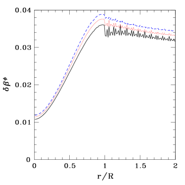
Figure 1: Relative error in $\beta^{\phi}$ along equatorial plane of star at $t=0$. Exact solutions from Cook et al. code CookPaper are compared to perturbative shift solver results at $T/|W|=2.43\times 10^{-3}$ (solid black lines), $4.9\times 10^{-3}$ (dashed blue lines), and $9.9\times 10^{-3}$ (dotted red lines). Here $\delta\beta^{\phi}\equiv(\beta^{\phi}_{\text{Cook}}-\beta^{\phi}_{\text{Pert}})/[(\beta^{\phi}_{\text{Cook}}+\beta^{\phi}_{\text{Pert}})/2]$. To demonstrate the approximate scaling $\delta\beta^{\phi}\propto T/|W|$, we have multiplied the value of $\delta\beta^{\phi}$ a factor of 4 for the case $T/|W|=2.43\times 10^{-3}$, and by a factor of 2 for the case $T/|W|=4.9\times 10^{-3}$.

To verify that our perturbative shift solver produces the shift $\beta^{\phi}$ accurately to order $\Omega$, we compute $\beta^{\phi}$ for differentially rotating, equilibrium star models and compare the results with those computed without approximation by the Cook et al. code CookPaper . Figure 1 shows the error, $\delta\beta^{\phi}$, for three models with the same central density ($\rho_{c}=1.54\times 10^{15}~{}(1.4M_{\odot}/M)^{2}~{}{\rm g}/{\rm cm}^{3}$) but with various $T/|W|$. We see that $\delta\beta^{\phi}$ decreases as $\Omega^{2}\propto T/|W|$, as expected. This shows that our perturbative shift solver accurately calculates $\beta^{\phi}$ to first order in $\Omega$.

V.2 Rigid Rotation Profile Study

When the star is uniformly rotating, a (weak) poloidal magnetic field should not change with time and it should have no effect on the star. To test our code, we evolve a uniformly rotating star with the physical parameters specified in Tables 2 and 3 (Rigid Rotation Profile Study). We follow the star for one Alfvén time ($\langle t_{A}\rangle=10.2P_{c}=4800M$). Figure 2 displays snapshots of the poloidal magnetic field in time, and Figure 3 shows the evolution of the rotational profile on the equatorial plane. As expected, neither the star’s rotation profile nor its magnetic field change significantly over the Alfvén timescale.

Figure 2: Snapshots of the poloidal magnetic field lines (contours of $A_{\phi}$) at $t/\langle t_{A}\rangle=0$, $0.5$, and $1.0$ for the uniformly rotating star. The field lines are drawn for $A_{\phi}=A_{\phi,\rm min}+(A_{\phi,\rm max}-A_{\phi,\rm min})i/20,~{}(i=1$–19), where $A_{\phi,\rm max}$ and $A_{\phi,\rm min}$ are the maximum and minimum values of $A_{\phi}$, respectively, at the given time. The dashed line in each plot indicates the initial stellar surface.

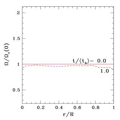
Figure 3: Snapshots of the rotation profile at the equatorial plane at $t/\langle t_{A}\rangle=0$ and $1.0$ for the uniformly rotating star.

VI Numerical Results

VI.1 MRI Resolution Study

Figure 4: $|B^{x}|_{\text{max}}$ vs. time, with perturbative results plotted on the left and nonperturbative (BSSN) on the right. Resolutions of $R/\Delta=75$, $100$, $150$, $200$, and $250$ are shown with solid, dotted, short dashed, long dashed, and long dash-dotted lines, respectively. The short dash-dotted line represents an approximate slope $\gamma=1/(5.0P_{c})$ for the exponential growth rate of the MRI, $\delta B^{x}\propto e^{\gamma t}$. Note that $\langle t_{A}\rangle/P_{c}=17.9$.

In the MRI Resolution Study, we perform simulations on a magnetized differentially rotating star (see Table 3) at resolutions $R/\Delta=75$, 100, 150, 200, and 250. The initial magnetic field is set so that $C=6.1\times 10^{-5}$. To demonstrate that the two metric solvers yield the same results, we also perform simulations with the BSSN metric solver at the two lowest resolutions ($R/\Delta=$75 and 100). Figure 4 displays the maximum magnitude of $|B^{x}|$ as a function of time. MRI causes the sudden increase of $|B^{x}|_{\rm max}$ at $t\approx 6P_{c}$. As resolution is increased, $|B^{x}|_{\rm max}$ saturates at larger values. Due to the turbulent nature of the MRI, we do not achieve convergence, even at the highest resolutions ($R/\Delta=200$ and 250). However the exponential growth time of the MRI, $\tau_{\text{MRI}}$, does converge at the highest resolutions ($R/\Delta=150\to 250$). The numerically determined value for $\tau_{\text{MRI}}$ is $\approx 5.0P_{c}$, which does not significantly deviate from the linearized, Newtonian theory estimate (obtained by applying Eq. (3) at $t=0$) of $\tau_{\text{MRI,min}}=5.7P_{c}$. We see that regardless of resolution or metric evolution scheme, the MRI-induced amplification of the magnetic field above its initial value becomes evident by $t\approx 6P_{c}$.

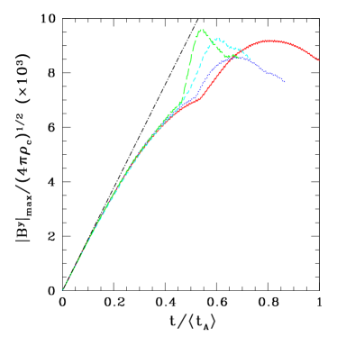
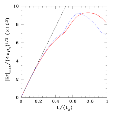
Figure 5: Evolution of $|B^{y}|_{\text{max}}(t)$. Simulations with resolution $R/\Delta=75$, $100$, $150$, and $250$ are shown with solid red, dotted blue, short dashed cyan, and long dashed green lines respectively, with perturbative results on the left and nonperturbative (BSSN) on the right. The dash-dotted black line represents the expected early-time linear growth of $|B^{y}|_{\rm max}$, as predicted by Eq. (2).

Figure 5 plots the maximum value of $|B^{y}|$ as a function of time. The straight lines in each plot indicate the expected growth rate via magnetic braking in the linear regime, according to Eq. (2). Notice that at early time, $|B^{y}|_{\text{max}}$ agrees well with the expected linear growth. However, the slope begins to flatten once the magnetic field becomes strong enough to induce fluid back-reaction. Later, the slope of $|B^{y}|_{\text{max}}$ increases once again before flattening at the point of saturation. As resolution is improved, the saturation point in $|B^{y}|_{\text{max}}$ occurs at earlier time. We find that the sudden increase in the slope correlates well with the increase of $|B^{x}|_{\text{max}}$ in the MRI plot of Figure 4. We also find that at the same time, the region at which $|B^{y}|_{\rm max}$ occurs shifts to the region where the MRI occurs. This is further evidence that the sudden increase in $|B^{y}|_{\text{max}}$ results from MRI-induced magnetic field rearrangement.

To further explore magnetic field rearrangement in our star at different resolutions, Figure 6 provides snapshots of poloidal magnetic field lines (i.e., contours of the vector potential $A_{\phi}$) at various times. Notice that MRI induces the largest distortion of the field lines in the outer equatorial region of the star. This is consistent with the linear analysis: Eq. (3), together with the star’s angular velocity profile, gives a shorter $\tau_{\rm MRI}$ near the outer part of the star. Similar behavior has been observed in simulations of magnetized, rapidly and differentially rotating stars MHDLett ; BigPaper . The distortion becomes more prominent at finer resolution, which suggests that more and more small-scale MRI modes are being resolved as resolution is improved.

Figure 6: Snapshots of poloidal magnetic field lines at various times, with resolution $R/\Delta=75$ (top), $150$, (middle), and $250$ (bottom). The field lines are drawn for $A_{\phi}=A_{\phi,\rm min}+(A_{\phi,\rm max}-A_{\phi,\rm min})i/20,~{}(i=1$–19), where $A_{\phi,\rm max}$ and $A_{\phi,\rm min}$ are the maximum and minimum values of $A_{\phi}$, respectively, at the given time. The dashed line in each plot indicates the initial stellar surface.

Next we analyze how the rotation profile of the star changes as a result of its magnetic field. Figure 7 shows the equatorial rotation profile at various times. Consistent with the results of StusFirst , we find that magnetic winding destroys the differential rotation profile on the Alfvén timescale, causing the star to rotate nearly as a solid body with $\Omega=\Omega_{\text{const}}$ at $t\approx 1\langle t_{A}\rangle$. Here $\Omega_{\text{const}}$ is the angular velocity of a uniformly rotating star with the same rest mass and angular momentum as the star under study. When the toroidal field saturates around $t\approx 1\langle t_{A}\rangle$, the magnetic fields begin to unwind, eventually causing the rotation profile to increase with increasing radius at roughly $2\langle t_{A}\rangle$. In addition, the MRI stirs up a turbulent-like flow, causing the bumpy rotation profile seen at later times.

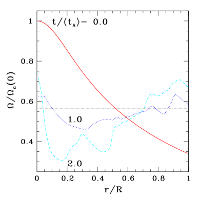
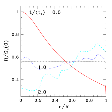
Figure 7: Rotation profile $\Omega$ measured in the equatorial plane at various times, comparing perturbative scheme (left) with nonperturbative (right) at $R/\Delta=75$ resolution. The straight line indicates the solid body angular frequency $\Omega_{\text{const}}$ of a star with the same angular momentum $J$ and rest mass $M_{0}$.

As the magnetic fields are wound, the magnetic energy $\mathcal{M}$ saps kinetic energy $T$ associated with differential rotation (Fig. 8) until the star rotates nearly as a solid body. At this point, we find that the star’s kinetic energy sinks to its minimum value shortly after $\mathcal{M}$ reaches maximum. Note that, consistent with Fig. 4, the maximum of $\mathcal{M}$ occurs earlier and earlier as resolution is improved due to an interplay between MRI and magnetic braking. After $\mathcal{M}$ reaches maximum, the fields unwind, pumping energy back into differential rotation, as shown at lowest resolutions in Fig. 8. We speculate, based on the $\alpha$-disk model MRIrev and on our previous work StusFirst ; JamesCookPaper ; MHDLett ; LiuShap , that the oscillations of $T$ and $\mathcal{M}$ will continue for many Alfvén times until the rotational kinetic energy associated with differential rotation is dissipated by phase mixing caused by MRI-induced turbulence. However, since the star is slowly rotating ($T/|W|=4.88\times 10^{-3}$) with weak magnetic fields ($\mathcal{M}\ll T$), the Alfvén time is long, $\langle t_{A}\rangle=10.2P_{c}=4800M$. It is therefore computationally taxing to accurately evolve the star for many Alfvén times, even if the perturbative metric solver is used.

As discussed in Section IV, perturbative metric solver initial data are only accurate to order $\Omega$. This causes oscillations to arise in our perturbative $T$ data at the level of $\Delta T\approx 0.0065$, where $\Delta T=[T-T(0)]/T(0)$ is the fractional deviation of the rotational kinetic energy from its initial value. The oscillations are evident in raw Fig. 8 perturbative data. A simple, local (in time) averaging technique is used to smooth out these oscillations in Fig. 8. Although they are smaller by an order of magnitude, we remove the oscillations in our perturbative $\mathcal{M}$ data as well, for consistency. Notice also in Fig. 8 that the value of $\mathcal{M}_{\text{max}}$ is comparable to that derived in Eq. (6).

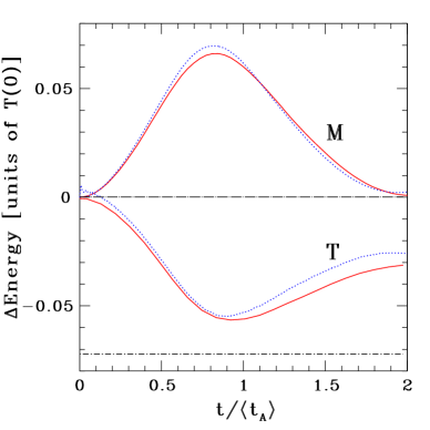
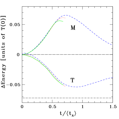
Figure 8: Rotational kinetic ($T$) and magnetic ($\mathcal{M}$) energies vs. time. For a given energy $E$, we define $\Delta E=[E(t)-E(0)]/T(0)$. The left plot compares results from the perturbative (solid red) and BSSN (dashed blue) metric algorithms at $R/\Delta=75$ out to $t=2\langle t_{A}\rangle$, and the right plot shows the same at $R/\Delta=100$ (perturbative: dotted red, BSSN: dashed blue) and $250$ (perturbative only: solid green). The rotational kinetic energy of rigid body rotation for the given $J$ is plotted at the bottom of each graph. The data for the perturbative runs have been smoothed to remove unphysical oscillations (see the text for details).

Figure 9 demonstrates that the angular momentum $J$ in our long-term simulations is well-conserved out to $2\langle t_{A}\rangle$. We see that angular momentum is lost at nearly a constant rate in our perturbative simulations, but the loss decreases with increasing resolution. In addition to angular momentum conservation, the binding energy $M_{0}-M_{\text{ADM}}$ is conserved to within $\approx 0.5\%$ in perturbative and $\approx 2.5\%$ in BSSN simulations.

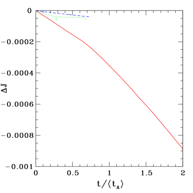
Figure 9: Relative change in angular momentum $J$ ($\Delta J=[J-J(0)]/J(0)$) vs. time at resolutions $R/\Delta=75$ (solid red), $150$ (dashed blue), and $250$ (dotted green). Recall that the $R/\Delta=250$ data is from a regridding run, where the data before $t/\langle t_{A}\rangle\approx 0.3$ is at $R/\Delta=100$, and $250$ after. This explains the varying slope in the $R/\Delta=250$ data. We plot results from the perturbative scheme only; the nonperturbative technique conserves $J$ to the same degree.

VI.2 $B$ Variation Study

In this study, the grid resolution is fixed at $R/\Delta=75$, and only the strength of the initial magnetic field is varied. We perform both perturbative and BSSN simulations. The MRI wavelengths in these simulation are $\langle\lambda_{\rm MRI}\rangle/\Delta=$3.6, 7.2, and 12.2. The corresponding magnetic field strength parameters are given in Table 2. Note that the last case is the same as the lowest resolution case in the “MRI Resolution Study”.

In Fig. 10, we plot $|B^{x}(t)|_{\text{max}}$ for the three magnetic field strengths. Although $\langle\lambda_{\text{MRI}}\rangle$ depends on initial magnetic field strength (Eq. (58)) , the MRI $e$-folding timescale $\tau_{\text{MRI}}$ does not (see, e.g. Eq. (3)). MRI is observed only when $\langle\lambda_{\text{MRI}}\rangle/\Delta\gtrsim 12$, which is consistent with the results of MHDLett ; BigPaper .

Figure 10: $|B^{x}|_{\text{max}}$ vs. time, with different initial magnetic field strengths, so that $\langle\lambda_{\text{MRI}}\rangle/\Delta=4.0$ (bottom line), 8.0 (middle line), and 12.2 (top line). Resolution is fixed at $R/\Delta=75$. Data from the perturbative spacetime evolution method are shown in the left plot, and BSSN method in the right.

VI.3 Rotation Profile Study

In this study, we consider a differentially rotating star in which $\Omega$ increases with cylindrical radius. We expect to see magnetic braking but not MRI in simulations of this star.

Figure 11 presents the same plots as those in Figs. 4–7 for this star. The top left plot indicates that, as expected, MRI is absent from this simulation. Although magnetic braking does appear (top right) as predicted, the curve is nearly parabolic and does not exhibit a sudden increase in slope as observed in Fig. 5. This further supports the notion that the sudden increase in slope in Fig. 5 results from an interplay between magnetic braking and MRI. Note also that the MRI-induced magnetic field distortion does not appear in the poloidal plane (middle three plots). Finally, we see that since the magnetic field-shifting effects of MRI are absent and the magnetic field is initially confined to the high density inner region of the star (Fig. 5), magnetic braking is incapable of flattening the rotation profile (bottom plot) in the less dense outer layers of the star.

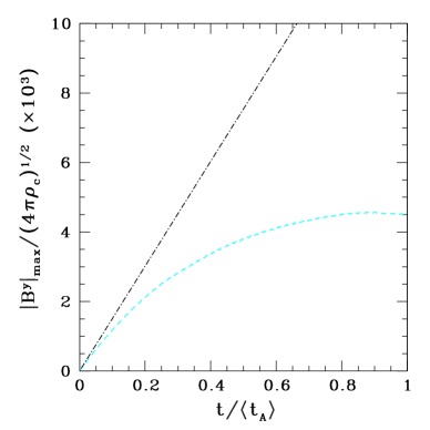
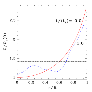
Figure 11: Results from the Rotation Profile Study. The plots from top left to bottom are analogues to Figure 4–7. Top left: $|B^{x}|_{\rm max}$ vs. time, top right: $|B^{y}|_{\rm max}$ vs. time, middle three plots: magnetic field lines (contours of $A_{\phi}$), bottom: equatorial rotation profile.

VII Conclusions

Our perturbative metric evolution algorithm yields results quite similar to those produced by the nonperturbative, BSSN-based evolution scheme. Because the outer boundary may be moved inward and the metric updated on a physically relevant timescale, perturbative metric simulations may be performed at $\sim 1/4$ the computational cost of BSSN metric simulations in axisymmetry for slowly rotating, weakly magnetized equilibrium stars. However, we found that loss of accuracy did occur after magnetic fields hit the outer boundary. This problem could be efficiently solved in future work by extending the outer boundary further from the star.

The stars we study in this paper are weakly magnetized ($\mathcal{M}/|W|\sim 10^{-6}$) and slowly rotating ($T/|W|\approx 0.005$). As a result, the Alfvén timescale is very long ($\sim 5000M$), and accurate simulations spanning many Alfvén times would be prohibitively expensive. In this paper, we reliably evolved such stars out to two Alfvén times at moderate resolution ($R/\Delta=75$). In these simulations, we found that magnetic fields wind and unwind on the Alfvén timescale, resulting in a trade-off between the kinetic energy in differential rotation and magnetic energy. Since we could not perform simulations spanning many Alfvén timescales while accurately resolving MRI, we can only speculate, based on the $\alpha$-disk model and our previous work StusFirst ; JamesCookPaper ; MHDLett ; LiuShap , that the oscillations between the magnetic and kinetic energy will be damped by MRI-induced dissipative processes over many Alfvén times.

In order to observe MRI in our simulations, we find that the spatial resolution must be set so that $\lambda_{\text{MRI}}/\Delta\gtrsim 10$, in agreement with the results of MHDLett ; BigPaper . We have also verified that MRI is not present if the star’s angular velocity initially increases with increasing distance from the rotation axis (i.e., the MRI is absent when $\partial_{\varpi}\Omega>0$).

We find that as resolution is increased, the effects of MRI become more and more prominent. Due to the turbulent nature of MRI, we do not achieve convergence of field amplitude, even if $\lambda_{\text{MRI}}/\Delta=32.6$ or $40.7$. However, we found the $e$-folding time of MRI, $\tau_{\rm MRI}$ does converge. The numerically determined value, $\tau_{\rm MRI}\approx 5.0P_{c}$ is consistent with the value predicted by the linearized, local Newtonian analysis ($5.72P_{c}$). The small difference is due in part to the fact that our star is relativistic. In addition, the linearized analysis assumes that $\lambda_{\rm MRI}$ is much smaller than the length scale on which the magnetic field changes (i.e. $\lambda_{\rm MRI}\ll B/|\nabla B|$), which is not quite satisfied in our magnetic field configuration.

Finally, we note that the behavior of the MRI is expected to be different in a full 3D calculation because of the effect of nonaxisymmetric MRI induced by a toroidal magnetic field. Turbulence may arise and persist more readily in 3D due to the lack of symmetry. More specifically, according to the axisymmetric anti-dynamo theorem hgb95 ; moffatt78 , sustained growth of the magnetic field energy is not possible through axisymmetric turbulence. Thus proper treatment of MRI in differentially rotating neutron stars requires high resolution simulations performed in full 3+1 dimensions. The computational cost of such simulations with existing 3+1 metric evolution schemes has thus far been prohibitive, but with our perturbative metric solver it may be possible to perform 3+1 simulations of weakly but realistically magnetized, slowly rotating stars at a small fraction of the computational cost.

Appendix A Derivation of Shift Equation (Eq. 16)

Here we derive the equation for the shift (Eq. 16), starting from the usual momentum constraint equation in the 3+1 ADM decomposition of Einstein’s field equations. Recall from Eq. (7) the perturbative line element is given by

$$ds^{2}=-e^{\nu(r)}dt^{2}+e^{\lambda(r)}dr^{2}+2\beta^{\phi}(t,r,\theta)r^{2}\sin^{2}{\theta}dtd\phi+r^{2}(\sin^{2}\theta d\phi^{2}+d\theta^{2})+\mathcal{O}(\Omega^{2})+\mathcal{O}(B^{2}).$$ (59)

We begin by writing the momentum constraint equation (Eq. 24 in ADM )

$$D_{j}K^{j}{}_{i}-D_{i}K=8\pi j_{i},$$ (60)

where $K=K^{j}{}_{j}$ and $j_{i}=-\gamma^{b}{}_{i}n_{c}T^{c}{}_{b}$. It can easily be shown from the ADM 3-metric evolution equation (Eq. 35 in ADM ) $\partial_{t}\gamma_{ij}=-2e^{\nu/2}K_{ij}+\mathcal{L}_{\beta}\gamma_{ij}$ that in this approximation $K_{ij}$ is given by

$$0=\partial_{t}\gamma_{ij}=-2e^{\nu/2}K_{ij}+\beta_{i|j}+\beta_{j|i}$$ (61)

where $\beta_{i|j}$ denotes the spatial covariant derivative $D_{j}\beta^{i}$, and the first equality reflects the stationarity of the 3-metric in this approximation. Taking the trace of this equation and applying the identity $\beta^{j}{}_{|j}=\frac{1}{\sqrt{\gamma}}(\sqrt{\gamma}\beta^{j})_{,j}$ (where $\gamma=\det{\gamma_{ij}}$) yields an expression for $K$:

$$-2e^{\nu/2}K+\frac{2}{\sqrt{\gamma}}(\sqrt{\gamma}\beta^{j})_{,j}=0.$$ (62)

Note that $(\sqrt{\gamma}\beta^{j})_{,j}=(\sqrt{\gamma}\beta^{\phi})_{,\phi}=0$ by axisymmetry, so Eq. (60) may be rewritten

$$K^{j}{}_{i|j}=8\pi j_{i}.$$ (63)

It follows from the definition of $j_{i}$ and the metric (59) that $j_{i}=e^{\nu/2}T^{0}{}_{i}$. We split the stress-energy tensor $T_{\mu\nu}$, as well as $j_{i}$, into a fluid part and an electromagnetic part:

$$T_{\mu\nu} = T^{\rm F}_{\mu\nu}+T^{\rm EM}_{\mu\nu}\ ,$$ (64)

$$T^{\rm F}_{\mu\nu} \equiv \rho_{0}hu_{\mu}u_{\nu}+Pg_{\mu\nu}\ ,$$ (65)

$$T^{\rm EM}_{\mu\nu} \equiv b^{2}u_{\mu}u_{\nu}+\frac{b^{2}}{2}g_{\mu\nu}-b_{\mu}b_{\nu}\ ,$$ (66)

$$j^{\rm F}_{i} = e^{\nu/2}T^{\rm F\,0}{}_{i}\ ,\ \ \ \ \ \ \ j^{\rm EM}_{i}=e^{\nu/2}T^{\rm EM\,0}{}_{i}\ .$$ (67)

Our approximation as summarized in Table 1 and derived in Appendix B ensures that $j^{\rm F}_{\phi}$ is the dominant component of $j_{i}$. In this approximation, $v^{i}=(0,0,\Omega)$ and

$$j_{\phi}=\rho_{o}he^{-\nu/2}(\Omega+\beta^{\phi})r^{2}\sin^{2}\theta.$$ (68)

Thus $i=\phi$ remains the only nonzero component of Eq. (63) to first order in $\Omega$ and $B$:

$$K^{j}{}_{\phi|j}=8\pi\rho_{o}he^{-\nu/2}(\Omega+\beta^{\phi})r^{2}\sin^{2}\theta\ .$$ (69)

Next we expand our expression for $K^{j}{}_{\phi|j}$:

$$K^{j}{}_{\phi|j} = \frac{1}{\sqrt{\gamma}}(\sqrt{\gamma}\,K^{j}{}_{\phi})_{,j}-\Gamma^{k}{}_{\phi m}K^{m}{}_{k}$$ (70)

$$= \frac{1}{\sqrt{\gamma}}(\sqrt{\gamma}\,r^{2}\sin^{2}\theta K^{j\phi})_{,j}-\Gamma^{k}{}_{\phi m}K^{ml}\gamma_{kl}.$$ (71)

It follows from Eq. (61) and the identity $\beta^{i}{}_{|j}=\beta^{i}{}_{,j}+\Gamma^{i}{}_{jk}\beta^{k}$ that

$$2e^{\nu/2}K^{ij}=(\beta^{i}{}_{,l}+\Gamma^{i}{}_{lk}\beta^{k})\gamma^{jl}+(\beta^{j}{}_{,l}+\Gamma^{j}{}_{lk}\beta^{k})\gamma^{il}.$$ (72)

After computing the necessary Christoffel symbols, we find that the nonvanishing components of $K^{ij}$ are:

$$K^{r\phi}=K^{\phi r} = \frac{1}{2e^{\nu/2}}\left(e^{-\lambda}\beta^{\phi}{}_{,r}\right)$$ (73)

$$K^{\theta\phi}=K^{\phi\theta} = \frac{1}{2e^{\nu/2}}\left(\frac{\beta^{\phi}{}_{,\theta}}{r^{2}}\right).$$ (74)

Plugging these expressions into Eqs. (71) and then (69) yields the equation governing the shift:

$$\frac{1}{r^{4}}[r^{4}j(r)\omega_{,r}]_{,r}+e^{\frac{\lambda-\nu}{2}}\frac{1}{r^{2}\sin^{3}{\theta}}[\sin^{3}{\theta}\omega_{,\theta}]_{,\theta}+\frac{4}{r}j^{\prime}(r)\omega=\frac{4}{r}j^{\prime}(r)\Omega,$$ (75)

where $\omega=-\beta^{\phi}$ and $j(r)=e^{-\frac{\lambda(r)+\nu(r)}{2}}$.

Finally, we perform the angular decompositions as in Eq. (17) and Eq. (18) and substitute them into Eq. (75) to obtain the equation

$$\frac{1}{r^{4}}\left[r^{4}j(r)\omega_{l}{}^{\prime}(r)\right]^{\prime}+\left[4\frac{j^{\prime}(r)}{r}-e^{(\lambda-\nu)/2}\frac{l(l+1)-2}{r^{2}}\right]\omega_{l}(r)=4\frac{j^{\prime}(r)}{r}\Omega_{l}(r).$$ (76)

This equation is the same as Eq. (30) in Hartle2 , which was derived using a different approach. Each $\omega_{l}$ must also satisfy the boundary conditions at the origin and at infinity (see below), as well as the matching conditions [Eqs. (22) and (23)] at the surface of the star.

A.1 Boundary condition at the origin

We now determine the boundary condition at the origin by analyzing the terms of Eq. (76) in the $r\rightarrow 0$ limit.

First we analyze $j(r)$ and its derivatives, starting with $j^{\prime}(0)=-\frac{1}{2}j(0)[\lambda^{\prime}(0)+\nu^{\prime}(0)]$. From the OV equations, we obtain

$$\lambda^{\prime}(0) = \left.\frac{2[rm^{\prime}(r)-m(r)]}{(r-2m(r))^{2}}\right|_{r\to 0}=0$$ (77)

$$\nu^{\prime}(0) = \left.\frac{2[m(r)+4\pi r^{3}P(r)]}{r[r-2m(r)]}\right|_{r\to 0}=0,$$ (78)

where we have used the expression $m(r)=(4/3)\pi r^{3}\rho(0)$ as $r\to 0$. Thus $j^{\prime}(0)=0$ since $j(r)=e^{-\frac{\lambda+\nu}{2}}$ is regular at $r=0$. Next we examine $j^{\prime}(r)/r$:

$$j^{\prime}(r)/r|_{r\to 0} = j^{\prime\prime}(0)=(e^{-\frac{\lambda+\nu}{2}})^{\prime\prime}|_{r\to 0}$$ (79)

$$= -\frac{1}{2}j(0)(\lambda^{\prime\prime}(r)+\nu^{\prime\prime}(r))|_{r\to 0}$$ (80)

$$= -\frac{1}{2}j(0)\left.\frac{d}{dr}\left\{\frac{2[rm^{\prime}(r)-m(r)]}{[r-2m(r)]^{2}}+\frac{2[m(r)+4\pi r^{3}P(r)]}{r[r-2m(r)]}\right\}\right|_{r\to 0}$$ (81)

$$= -\frac{4}{3}\pi j(0)[4\rho(0)+3P(0)].$$ (82)

We may therefore write Eq. (76) near $r\to 0$ as follows

$$\omega_{l}^{\prime\prime}(r)+\frac{4}{r}\omega_{l}^{\prime}(r)+4\omega_{l}(r)\frac{j^{\prime\prime}(0)}{j(0)}-\frac{l(l+1)-2}{r^{2}}\omega_{l}(r)=4\Omega_{l}(0)\frac{j^{\prime\prime}(0)}{j(0)},$$ (83)

with solution given by Eq. (20).

A.2 Boundary condition at infinity

Outside the star, $P=\rho=0$ and the time independent (diagonal) metric becomes Schwarzschild, so $e^{\nu}=e^{-\lambda}=1-2M/r$. The ODE governing the shift outside the star is therefore given by

$$\frac{1}{r^{4}}[r^{4}\omega_{l}{}^{\prime}(r)]^{\prime}-\frac{1}{1-2M/r}\frac{l(l+1)-2}{r^{2}}\omega_{l}(r)=0.$$ (84)

Since $2M/r\ll 1$ in the limit $r\to\infty$, we may write Eq. (76) as

$$\frac{1}{r^{4}}\frac{d}{dr}(r^{4}\frac{d\omega_{l}}{dr})-\frac{l(l+1)-2}{r^{2}}\omega_{l}=0$$ (85)

with solution given by Eq. (21).

Note that the analytic solution for Eq. (84) exists and is given in terms of the hypergeometric function:

$$\omega_{l}=\begin{cases}\displaystyle\frac{C_{1}}{r^{3}},&\text{if }l=1,\text{and}\cr\cr\displaystyle\frac{C_{l}}{r^{l+2}}{{}_{2}F_{1}}(l+2,l-1;2l+2;2M/r),&\text{otherwise}.\end{cases}$$ (86)

A.3 Rigid rotation case

In the case of solid body rotation ($\Omega(r,\theta)=\text{constant}$), only the $l=1$ mode in Eq. 19 contributes to $\Omega$. Thus the right-hand side of Eq. (76) is zero for $l>1$. For $l>1$, the solution $\omega_{l}=0$ satisfies the boundary conditions at the origin and at infinity [Eqs. (20) and (21)] and the matching conditions at the stars’s surface [Eqs. (22) and (23)], so $\omega_{l}=0$ is the solution for $l>1$. This coincides with the result cited in Hartle .

Appendix B Derivation of Slow Rotation Approximation Inequalities

In this section, we derive inequalities that must hold in order for our primary assumption in Appendix A [leading to Eq. (68)] to be valid.

We have assumed that the metric can be written in the form (7) at all times, with the shift $\beta^{\phi}=-\omega$ being the only non-diagonal component of the metric. For this to be true, the system has to be (approximately) stationary, axisymmetric and the stress-energy tensor has to be circular or nonconvective circular :

$$\epsilon_{\alpha}T^{\alpha[\beta}\epsilon^{\gamma}\xi^{\delta]} = 0\ ,$$ (87)

$$\xi_{\alpha}T^{\alpha[\beta}\epsilon^{\gamma}\xi^{\delta]} = 0\ ,$$ (88)

where $\epsilon=\partial/\partial t$ and $\xi=\partial/\partial\phi$ are two Killing vector fields associated with stationarity and axisymmetry, respectively. These circularity conditions are satisfied if the momentum currents in the meridional planes are negligible compared with the axial component. Hence we require that

$$|j_{\hat{\phi}}|\gg|j_{\hat{r}}|\ \ \ \ \mbox{and}\ \ \ \ |j_{\hat{\phi}}|\gg|j_{\hat{\theta}}|\ ,$$ (89)

where the “hats” denote the orthonormal components.

We split the stress-energy tensor into a fluid part and an electromagnetic part: $T^{\mu\nu}=T^{\mu\nu}_{\rm F}+T^{\mu\nu}_{\rm EM}$, where

$$T^{\mu\nu}_{\rm F} = \rho_{0}hu^{\mu}u^{\nu}+Pg^{\mu\nu}\ ,$$ (90)

$$T^{\mu\nu}_{\rm EM} = b^{2}u^{\mu}u^{\nu}+\frac{b^{2}}{2}g^{\mu\nu}-b^{\mu}b^{\nu}\ .$$ (91)

From this we obtain the following expressions for $T^{0}{}_{i}{}^{\text{F}}$ and $T^{0}{}_{i}{}^{\text{\rm EM}}$:

$$T^{0}{}_{i}{}^{\text{F}} = \rho_{0}hu^{0}u_{i}$$ (92)

$$= \rho_{0}h(u^{0})^{2}\gamma_{ij}(v^{j}+\beta^{j})$$ (93)

$$\sim \rho_{0}he^{-\nu}\gamma_{ij}v^{j}\ ,$$ (94)

$$T^{0}{}_{i}{}^{\text{EM}} = b^{2}u^{0}u_{i}-b^{0}b_{i}$$ (95)

$$\sim e^{-\nu}\,\frac{v^{j}}{4\pi}(\gamma_{ij}B^{2}-B_{i}B_{j})\ ,$$ (96)

where we have used the fact that $v^{j}+\beta^{j}\sim v^{j}$ and $\alpha u^{0}=1+O(\Omega^{2})$ for slowly rotating stars. Here the lapse $\alpha=e^{\nu/2}$.

Since $j_{i}=e^{\nu/2}T^{0}{}_{i}$, we may split the momentum current density in the same way: $j_{i}=j^{\rm F}_{i}+j^{\rm EM}_{i}$. Using the above expression for $T^{0}{}_{i}^{\text{F}}$ and the metric (7), we find

$$j_{i}^{\text{F}}=e^{\nu/2}T^{0}{}_{i}{}^{\text{F}}\implies\begin{cases}\displaystyle j_{\hat{\phi}}^{\text{F}}\sim e^{-\nu/2}\rho_{0}hr\Omega\cr\displaystyle j_{\hat{\theta}}^{\text{F}}\sim\left(\frac{v^{\hat{\theta}}}{\Omega r}\right)j_{\hat{\phi}}^{\text{F}}\cr\displaystyle j_{\hat{r}}^{\text{F}}\sim e^{-\lambda/2}\left(\frac{v^{\hat{r}}}{\Omega r}\right)j_{\hat{\phi}}^{\text{F}}\end{cases}\ .$$ (97)

In the absence of magnetic fields, $j_{i}=j_{i}^{\rm F}$ and the conditions (89) yield $|v^{\hat{\theta}}|\ll|\Omega|r$ and $|v^{\hat{r}}|\ll|\Omega|r$ [Assuming $e^{-\lambda/2}\sim O(1)$]. Applying these inequalities, the electromagnetic part of $j_{i}$ becomes

$$j_{i}^{\text{EM}}=e^{\nu/2}T^{0}{}_{i}{}^{\text{EM}}\implies\begin{cases}\displaystyle j_{\hat{\phi}}^{\text{EM}}\sim\frac{B^{2}-(B^{\hat{\phi}})^{2}}{4\pi\rho_{0}h}\displaystyle j_{\hat{\phi}}^{\text{F}}\cr\displaystyle j_{\hat{\theta}}^{\text{EM}}\sim\frac{B^{2}}{4\pi\rho_{0}h}\left[\frac{v^{\hat{\theta}}}{\Omega r}\left(1-\frac{(B^{\hat{\theta}})^{2}}{B^{2}}\right)-\frac{B^{\hat{\theta}}B^{\hat{\phi}}}{B^{2}}\right]\displaystyle j_{\hat{\phi}}^{\text{F}}\cr\displaystyle j_{\hat{r}}^{\text{EM}}\sim\frac{B^{2}}{4\pi\rho_{0}h}e^{-\lambda/2}\left[\frac{v^{\hat{r}}}{\Omega r}\left(1-e^{-\lambda}\frac{(B^{\hat{r}})^{2}}{B^{2}}\right)-\frac{B^{\hat{r}}B^{\hat{\phi}}}{B^{2}}\right]\displaystyle j_{\hat{\phi}}^{\text{F}}\end{cases}\ .$$ (98)

For simplicity, we have ignored the magnetic field terms when computing the shift in Appendix A. For this to be valid, we need to impose an additional condition:

$$|j_{\hat{\phi}}^{\text{F}}|\gg|j_{\hat{\phi}}^{\text{EM}}|\ .$$ (99)

Equations (97) and (98) together with the conditions (89) and (99) yield the following inequalities which must be satisfied for the shift equations in Appendix A to be valid:

$$\left|\frac{v^{\hat{r}}}{\Omega r}\right|\ll 1\ ,\ \ \ \ \ \left|\frac{v^{\hat{\theta}}}{\Omega r}\right|\ll 1\ ,\ \ \ \ \ \frac{(B^{\hat{r}})^{2}}{4\pi\rho_{0}h}\ll 1\ ,\ \ \ \ \ \frac{(B^{\hat{\theta}})^{2}}{4\pi\rho_{0}h}\ll 1\ ,\text{ and}\ \ \ \ \ \frac{(B^{\hat{\phi}})^{2}}{4\pi\rho_{0}h}\lesssim 1\ .$$ (100)

For information on how well these inequalities are satisfied in our simulations, see Table I.

References

- (1) V. P. Velikhov, Soc. Phys. JETP 36, 995 (1959); S. Chandrasekhar, Proc. Natl. Acad. Sci. USA 46, 253 (1960).
- (2) S. A. Balbus and J. F. Hawley, Astrophys. J. 376, 214 (1991).
- (3) F. A. Rasio and S. L. Shapiro, Astrophys. J. 432, 242 (1994); Class. Quant. Grav. 16 R1 (1999).
- (4) T. W. Baumgarte, S. L. Shapiro, and M. Shibata, Astrophys. J. Lett. 528, L29 (2000).
- (5) M. Shibata and K. Uryu, Phys. Rev. D 61, 064001 (2000); M. Shibata and K. Uryu, Prog. Theor. Phys. 107, 265 (2002); M. Shibata, K. Taniguchi, and K. Uryu, Phys. Rev. D 68, 084020, (2003); M. Shibata and K. Taniguchi, Phys. Rev. D 73, 064027 (2006).
- (6) T. Zwerger and E. Müller, Astron. Astrophys. 320, 209 (1997); M. Ruffert and H.-T. Janka, Astron. Astrophys. 344, 573 (1999).
- (7) Y. T. Liu and L. Lindblom, Mon. Not. R. Astron. Soc. 324, 1063 (2001); Y. T. Liu, Phys. Rev. D 65, 124003 (2002).
- (8) S. L. Shapiro, Astrophys. J. 544, 397 (2000).
- (9) T. C. Mouschovias and E. V. Paleologou, Astrophys. J. 230, 204 (1979); T. C. Mouschovias and E. V. Paleologou, Astrophys. J. 237, 877 (1980).
- (10) J. N. Cook, S. L. Shapiro, and B. C. Stephens, Astrophys. J. 599, 1272 (2003).
- (11) Y. T. Liu and S. L. Shapiro, Phys. Rev. D 69, 044009 (2004).
- (12) H. C. Spruit, Astron. Astrophys. 349, 189 (1999).
- (13) M. D. Duez, Y. T. Liu, S. L. Shapiro, M. Shibata, and B. C. Stephens, Phys. Rev. D 73, 104015 (2006).
- (14) M. D. Duez, Y. T. Liu, S. L. Shapiro, M. Shibata, and B. C. Stephens, Phys. Rev. Lett. 96, 031101 (2006).
- (15) M. Shibata, M. D. Duez, Y. T. Liu, S. L. Shapiro, and B. C. Stephens, Phys. Rev. Lett. 96, 031102 (2006).
- (16) M. D. Duez, Y. T. Liu, S. L. Shapiro, and B. C. Stephens, Phys. Rev. D 72, 024028 (2005)
- (17) M. Shibata and Y.-I. Sekiguchi, Phys. Rev. D 72, 044014 (2005).
- (18) J. B. Hartle, Astrophys. J. 150, 1005 (1967).
- (19) J. B. Hartle, Astrophys. J. 161, 111 (1970).
- (20) M. Shibata and T. Nakamura, Phys. Rev. D 52, 5428 (1995); T. W. Baumgarte and S. L. Shapiro, Phys. Rev. D 59, 024007 (1998).
- (21) S. A. Balbus and J. F. Hawley, Rev. Mod. Phys. 70, 1 (1998).
- (22) T. W. Baumgarte, S. L. Shapiro, and M. Shibata, Astrophys. J. Lett. 528, L29 (2000).
- (23) J. R. Oppenheimer and G. Volkoff, Phys. Rev. 55, 374 (1939).
- (24) J. W. York, in Sources of Gravitational Radiation, edited by L. Smarr (Cambridge University Press, 1979).
- (25) M. Alcubierre, B. Brügmann, D. Pollney, E. Seidel, and R. Takahashi, Phys. Rev. D 64, 061501(R) (2001).
- (26) M. D. Duez, S. L. Shapiro, and H.-J. Yo, Phys. Rev. D 69 104016 (2004).
- (27) M. Alcubierre, S. Brandt, B. Brügmann, D. Holz, E. Seidel, R. Takahashi, and J. Thornburg, Int. J. Mod. Phys. D10, 273 (2001).
- (28) P. Colella and P. R. Woodward, J. Comput. Phys., 54, 174 (1984).
- (29) A. Harten, P. D. Lax, and B. van Leer On Upstream Differencing and Godunov-Type Schemes for Hyperbolic Conservation Laws, SIAM Rev., 25, 35-61, (1983).
- (30) G. B. Cook, S. L. Shapiro, and S. A. Teukolsky, Astrophys. J. 398, 203 (1992).
- (31) J. F. Hawley, C. F. Gammie, and S. A. Balbus, Astrophys. J. 440, 742 (1995); J. F. Hawley, Astrophys. J. 528, 462 (2000).
- (32) H. K. Moffatt, Magnetic Field Generation in Electrically Conducting Fluids (Cambridge Univ. Press, 1978).
- (33) B. Carter, in Black Holes – Les Houches 1972, edited by C. DeWitt and B. S. DeWitt (Gordon and Breach, New York, 1973); A. Papapetrou, Ann. Inst. H. Poincaré A 4, 83 (1966); B. Carter, J. Math. Phys. 10, 70 (1969); E. Gourgoulhon, and S. Bonazzola, Phys. Rev. D 48, 2635 (1993).