Quest for circular polarization of gravitational wave background and orbits of laser interferometers in space

Abstract

We show that isotropic component of circular polarization of stochastic gravitational wave background can be explored by breaking two dimensional configuration of multiple laser interferometers for correlation analysis. By appropriately selecting orbital parameters for the proposed BBO mission, the circular polarization degree $\Pi$ can be measured down to $\Pi\sim 0.08(\Omega_{GW}/10^{-15})^{-1}(SNR/5)$ with slightly ($\sim 10\%$) sacrificing the detection limit for the total intensity $\Omega_{GW}$ compared to the standard plane symmetric configuration. This might allow us to detect signature of parity violation in the very early universe.

I introduction

Due to extreme penetrating power of gravitational waves, observation of the waves may enable us to study the very early universe in a way that cannot be achieved with other methods Allen:1996vm . Recently, follow-on missions to the Laser Interferometer Space Antenna (LISA) lisa have been actively discussed to directly detect stochastic gravitational wave background from the early universe around $\sim 1$Hz. The primary target for the proposed missions, such as, the Big Bang Observer (BBO) bbo and DECIGO Seto:2001qf , is the gravitational wave background produced at inflation. With various observational supports for inflation, existence of the background is plausible, while it is currently difficult to predict its amplitude.

Meanwhile, considering the facts that observation of gravitational waves will be a truly new frontier of cosmology and our understanding of physics is limited at very high energy scale, it would be quite meaningful to prepare flexibly to various observational possibilities. Actually, detection of something unexpected with odd properties will be generally more exciting than confirmation of something widely anticipated. For this purpose it is preferable that we can study gravitational wave background beyond its simple spectral information, and model independent approach would be effective with regard to the sources of the background.

One of fundamental as well as interesting properties of the background is its circular polarization. Circular polarization characterizes asymmetry of amplitudes of right- and left-handed waves, and its generation is expected to be closely related to parity violation (see e.g. Lue:1998mq ). In a recent paper p1 it was shown that LISA can measure the dipole ($l=1$) and octupole ($l=3$) anisotropic patterns of circular polarization of the background in a relatively clean manner, but, at the same time, LISA cannot capture its monopole ($l=0$) mode due to a symmetric reason. Since our observed universe is highly homogeneous and isotropic at cosmological scales, it would be essential to have sensitivity to the monopole mode of circular polarization of cosmological background. The proposed missions like BBO or DECIGO are planed to use multiple sets of interferometers to perform correlation analysis to measure the total intensity $\Omega_{GW}$ of cosmological background by beating out detector noises with a long-term signal integration. The standard configuration of these missions is to put the multiple interferometers on a same plane. This is advantageous to get a good sensitivity to the total intensity $\Omega_{GW}$, as a larger spatial separation between interferometers results in reducing their overlapped responses to gravitational waves Flanagan:1993ix . However, with this plane symmetric configuration, we are totally blind to the monopole mode of circular polarization, as in the case of LISA. This means that even if the isotropic background is circularly polarized by 100%, we will not be able to discriminate its extreme nature. In this paper we study how well we can detect the monopole mode of circular polarization by breaking symmetry of the detector configuration.

II circular polarization

In the transverse-traceless gauge, the metric perturbation due to gravitational waves is expressed by superposition of plane waves as follows:

$$h_{ab}(t,{\mbox{\boldmath${x}$}})=\sum_{P=+,\times}\int^{\infty}_{-\infty}df\int_{S^{2}}d\mbox{\boldmath${n}$}~{}h_{P}(f,\mbox{\boldmath${n}$})e^{2\pi if(t-\mbox{\boldmath${n}$}\cdot{\mbox{\boldmath${x}$}})}{\mbox{\boldmath${e}$}}^{P}_{ab}(\mbox{\boldmath${n}$}),$$ (1)

where $S^{2}$ is the unit sphere for the angular integral, the unite vector $\mbox{\boldmath${n}$}=(\sin\theta\cos\phi,\sin\theta\sin\phi,\cos\theta)$ is propagation direction of the waves, and ${\mbox{\boldmath${e}$}}^{+}_{ab}$ and ${\mbox{\boldmath${e}$}}^{\times}_{ab}$ are the bases for transverse-traceless tensors. We fix them as ${\mbox{\boldmath${e}$}}^{+}={\hat{\mbox{\boldmath${e}$}}}_{\theta}\otimes{\hat{\mbox{\boldmath${e}$}}}_{\theta}-{\hat{\mbox{\boldmath${e}$}}}_{\phi}\otimes{\hat{\mbox{\boldmath${e}$}}}_{\phi}$ and ${\mbox{\boldmath${e}$}}^{\times}={\hat{\mbox{\boldmath${e}$}}}_{\theta}\otimes{\hat{\mbox{\boldmath${e}$}}}_{\phi}+{\hat{\mbox{\boldmath${e}$}}}_{\phi}\otimes{\hat{\mbox{\boldmath${e}$}}}_{\theta}$ where two unit vectors ${\hat{\mbox{\boldmath${e}$}}}_{\theta}$ and ${\hat{\mbox{\boldmath${e}$}}}_{\phi}$ are defined in a fixed spherical coordinate system, as usual. The frequency dependence is easily resolved by Fourier transformation, and we omit its explicit dependence for notational simplicity, unless we need to keep it. We decompose the covariance matrix $\left\langle h_{P1}(\mbox{\boldmath${n}$})h_{P2}^{*}(\mbox{\boldmath${n}$}^{\prime})\right\rangle$ $(P1,P2=+,\times)$ for two polarization modes as

$$\frac{\delta_{drc}(\mbox{\boldmath${n}$}-\mbox{\boldmath${n}$}^{\prime})}{4\pi}\left(\begin{array}[]{@{\,}cc@{\,}}I(\mbox{\boldmath${n}$})+Q(\mbox{\boldmath${n}$})&U(\mbox{\boldmath${n}$})-iV(\mbox{\boldmath${n}$})\\ U(\mbox{\boldmath${n}$})+iV(\mbox{\boldmath${n}$})&I(\mbox{\boldmath${n}$})-Q(\mbox{\boldmath${n}$})\\ \end{array}\right),$$ (2)

where $I,Q,U$ and $V$ are the Stokes parameters and are real by definition. The parameters $Q$ and $U$ are related to linear polarization, and their combinations $Q\pm iU$ have spin $\pm 4$ and are expanded in terms of the spin-weighted spherical harmonics ${}_{\pm 4}Y_{lm}(\mbox{\boldmath${n}$})$ defined for $l\geq 4$ p1 . Therefore, they do not have modes naturally corresponding to the monopole pattern. The parameter $I$ represents the total intensity, while the parameter $V$ shows asymmetry of amplitudes of right- and left-handed waves. These meanings become apparent with using the circular polarization bases ${\mbox{\boldmath${e}$}}_{R,L}=({\mbox{\boldmath${e}$}}_{+}\pm i{\mbox{\boldmath${e}$}}_{\times})/\sqrt{2}$ for which the expansion coefficients become $h_{R,L}=(h_{+}\mp ih_{\times})/\sqrt{2}$. The parameters $I$ and $V$ can be expressed as $I(\mbox{\boldmath${n}$})=\left\langle|h_{R}|^{2}+|h_{L}|^{2}\right\rangle/2=\left\langle|h_{+}|^{2}+|h_{\times}|^{2}\right\rangle/2$ and $V(\mbox{\boldmath${n}$})=\left\langle|h_{R}|^{2}-|h_{L}|^{2}\right\rangle/2=i\left\langle h_{+}h_{\times}^{*}-h_{+}^{*}h_{\times}\right\rangle/2$. They are spin 0 quantities and have monopole modes $I_{00}$ and $V_{00}$ for spherical harmonic expansions $I(\mbox{\boldmath${n}$})=\sum_{lm}I_{lm}Y_{lm}(\mbox{\boldmath${n}$})$ and $V(\mbox{\boldmath${n}$})=\sum_{lm}V_{lm}Y_{lm}(\mbox{\boldmath${n}$})$. In this paper we mainly discuss how to capture the monopole mode of circular polarization signal $V_{00}$ with laser interferometers in space.

To begin with, we summarize basic aspects of LISA lisa . LISA is formed by three spacecrafts that nearly keep a regular triangle with its side length $L=5\times 10^{6}$km. The geometric barycenter of the triangle moves on a circular orbit around the Sun with radius $\sim 1$AU. The detector plane made by the triangle inclines to the orbital plane of the barycenter by $\sim 60^{\circ}$ with changing its orientation. The triangle also rotates annually on the detector plane (the so-called “cartwheel motions”). From its six one-way relative frequency fluctuations of the laser light, we can make three Time-Delay-Interferometer (TDI) variables $\left\{A,E,T\right\}$ that cancel the laser frequency noises Prince:2002hp . The detector noises between these three variables are not correlated due to a symmetry of the data streams, and two modes $\left\{A,E\right\}$ have similar noise spectra Prince:2002hp . At low frequency regime ${\hat{f}}\equiv 2\pi f/L\ll 1$, the responses of two modes $\left\{A,E\right\}$ to gravitational waves can be regarded as those of two simple L-shaped interferometers that measure differences of two arm-lengths caused by passing gravitational waves, as shown in figure 1. The $T$-mode is less sensitive to gravitational waves at ${\hat{f}}\lesssim 1$ and is not important in this paper (see e.g. Seto:2005qy ; Corbin:2005ny ). Since the monopole modes $I_{00}$ and $V_{00}$ are our main concern and they are invariant under rotation of a coordinate system, we only use the coordinate system $XYZ$ fixed to the single system B1 as shown in figure 1. These basic aspects for LISA are essentially same for BBO bbo . But BBO is planed to have a smaller arm-length $L=5\times 10^{4}$km (${\hat{f}}=1$ corresponding to 0.95Hz) and use multiple systems (triangles) not only the first system B1 bbo (see also Seto:2005qy ; Corbin:2005ny ). The responses of $A$ and $E$ modes to gravitational waves are written as

$$\left\{A,E\right\}=\int_{S^{2}}d\mbox{\boldmath${n}$}\sum_{P=+,\times}h_{P}(\mbox{\boldmath${n}$})F^{p}_{\left\{A,E\right\}}(\mbox{\boldmath${n}$},{\hat{f}}),$$ (3)

and the pattern functions $F^{P}_{A}(\mbox{\boldmath${n}$},f)$ for $A$ mode are expressed as $F_{A}^{+}(\mbox{\boldmath${n}$},f)=\frac{1}{2}(1+\cos^{2}\theta)\sin(2\phi)+O({\hat{f}})$ and $F_{A}^{\times}(\mbox{\boldmath${n}$},f)=\cos\theta\cos(2\phi)+O({\hat{f}})$ (see e.g. Taruya:2006kq ; Seto:2002uj ). The functions $F^{P}_{E}(\mbox{\boldmath${n}$},f)$ for $E$ mode is given by replacing $\phi$ with $\phi+\pi/4$. Here we multiplied an appropriate common factor proportional to some powers of ${\hat{f}}$ so that the pattern functions become the simple form at the low frequency limit ${\hat{f}}\to 1$ as presented above. This normalization is just for illustrative purpose and not essential for our study. Note that we have correspondences such as $F_{A}^{+}\to F_{A}^{+}$ and $F_{A}^{\times}\to-F_{A}^{\times}$ at order $O({\hat{f}}^{0})$ for a plane symmetric replacement $\theta\to\pi/2-\theta$ and $\phi\to\phi$. These are indeed valid at any order $O({\hat{f}}^{n})$ (see e.g. IV.C in Taruya:2006kq ), as we can expect from simple geometric consideration.

With data streams $A$ and $E$ from a single system B1 we can make three meaningful combinations $AA^{*}$, $EE^{*}$ and $AE^{*}$. The expectation values for a combination $C$ by the monopole modes $I_{00}$ and $V_{00}$ can be written as

$$\left\langle C(f)\right\rangle=\left[\gamma_{I,C}(f)I_{00}(f)+\gamma_{V,C}(f)V_{00}(f)\right]/5.$$ (4)

The overlap functions $\gamma_{\left\{I,V\right\},C}$ show the relative strength of inputs $I_{00}$ and $V_{00}$ to an observable $\left\langle C\right\rangle$ Flanagan:1993ix . They are given by the pattern functions, such as, $F_{A}^{+}(\mbox{\boldmath${n}$},{\hat{f}})$ and $F_{A}^{\times}(\mbox{\boldmath${n}$},{\hat{f}})$ . For example, the function $\gamma_{V,AE^{\prime*}}$ for $C=AE^{*}$ is given by

$$\gamma_{V,AE*}(f)=\frac{5}{4\pi}\int_{S^{2}}d\mbox{\boldmath${n}$}\left[i\left\{F_{A}^{+}F_{E}^{\times*}-F_{A}^{\times}F_{E}^{+*}\right\}\right].$$ (5)

Here we used the definition (2) and equation (3). In a same manner the function $\gamma_{I,AA^{\prime*}}$ is given by replacing the above parenthesis $[\cdots]$ with $\left[F_{A}^{+}F_{A}^{+*}+F_{A}^{\times}F_{A}^{\times*}\right]$. The kernel $[\cdots]$ for $\gamma_{V,AE^{\prime}*}$ at order $O({\hat{f}}^{0})$ is given by

$$-i\left(\frac{1+\cos^{2}\theta}{2}\right)\cos\theta.$$ (6)

This factor is decomposed only with dipole $(l=1)$ and octupole $(l=3)$ patterns p1 , and cannot probe the monopole $V_{00}$. This is because responses of interferometers to incident waves have an apparent symmetry with respect to the detector plane, and this cancellation holds at any order $O({\hat{f}}^{n})$ (see e.g. IV.C in Taruya:2006kq ). From the same reason we cannot probe the mode $V_{00}$ with using self correlation, such as $\left\langle AA^{*}\right\rangle$ or $\left\langle EE^{*}\right\rangle$. We need independent data streams to capture the target $V_{00}$. Note that the kernel for $\gamma_{I,AE^{*}}$ becomes $8^{-1}(1-\cos^{2}\theta)^{2}\sin 4\phi$ at $O({\hat{f}}^{0})$. It is written only with hexadecapole modes $(l=4)$ Taruya:2006kq ; Seto:2004np , and we have $\gamma_{I,AE^{*}}=0$ at $O({\hat{f}}^{0})$. As we see later, this is preferable to reduce the contamination of $I_{00}$ to determine the target $V_{00}$ with using a combination that is a refined version of $AE^{*}$.

Next we consider a second system B2 in addition to the first one B1 discussed so far. With the standard configuration of BBO, B2 is put at position obtained by rotating B1 around the $Z$-axis by $180^{\circ}$, and arms of these two systems form a star-like shape on the $XY$-plane bbo ; Seto:2005qy ; Corbin:2005ny . But as discussed above, we can not capture $V_{00}$ with this configuration due to the plane symmetry of interferometers. Therefore, we study a simple case with breaking this symmetry. We consider to put B2 (more precisely its barycenter) on a circular orbit that has the same radius ($\sim 1$AU) as B1, but its orbital plane is inclined to that of B1 with an angle $\varepsilon=D/{\rm 1AU}\lesssim 10^{-3}$ in units of radian. Here the parameter $D$ is the maximum distance between barycenters of B1 and B2, and its preferable scale is $\sim 10^{5}$km, namely the same order as the arm-length $L$ of BBO, as we see later. The two orbits of the barycenters intersect twice per orbital period $T_{orb}(\sim 1{\rm yr})$. In figure 2 their configurations are shown with viewing from their node. We neglect tiny misalignment of directions of two detector planes of order $\varepsilon$, and only study effects caused by their relative positions. By dealing with the rotation of detector planes and the cartwheel motions mentioned earlier, we can follow the position of the B2’s barycenter on the moving $XYZ$-coordinate attached to B1. The trajectory of B2’s barycenter $(B_{X},B_{Y},B_{Z})$ is given as

$$d_{X} \equiv B_{X}/L=\sqrt{3}d(\cos\omega\cos(\omega+\alpha))/2,$$ (7)

$$d_{Y} \equiv B_{Y}/L=\sqrt{3}d(\cos\omega\sin(\omega+\alpha))/2,$$ (8)

$$d_{Z} \equiv B_{Z}/L=d\cos\omega/2.$$ (9)

Here we have defined $d\equiv{D}/L$, and the parameter $\omega=2\pi(t/T_{orb})$ is the orbital phase of B1 around the Sun. In figure 1 we show the trajectory of B2 for $(\alpha,d)=(0,0.24)$ as dotted curves. The standard BBO configuration is recovered with putting $d=0$. The free parameter $\alpha$ determines the orientation the dotted curves around the $Z$-axis, and we hereafter fix it at $\alpha=0$.

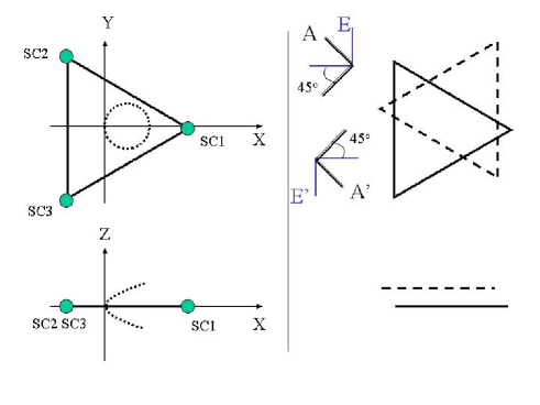
Figure 1: Three spacecrafts (SCs) of a LISA-type system (B1) are shown with circles that are put on the $XY$-plane. The barycenter of three SCs is at the origin $(X,Y,Z)=(0,0,0)$. The bottom figure shows the projection of the structures to the $XZ$-plane. At low frequency limit the responses of two TDI modes $A$ and $E$ can be effectively regarded as those of two L-shaped interferometers with shown orientations. On the coordinate system $(X,Y,Z)$ fixed to the first system B1, the center of the second system B2 moves on the the dotted curves for the specific parameter choice $(\alpha,d)=(0,0.24)$. A typical snapshot of B1 (solid line) and B2 (dashed line) is shown on the right side. The orientations of two effective L-shaped interferometers for $A^{\prime}$ and $E^{\prime}$ modes are also given.

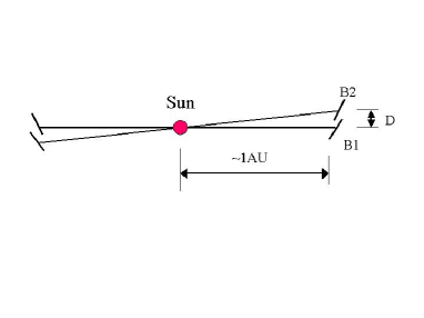
Figure 2: Configuration of two orbital planes for B1 and B2 seen from their node (orbital phase: $\omega=\pi/2$).

We define two TDI modes $A^{\prime}$ and $E^{\prime}$ made from B2 system in the same way as $A$ and $E$ from B1. Now two modes $A^{\prime}$ and $E^{\prime}$ are not on the $XY$-plane (except for $\omega=\pi/2,3\pi/2,\cdots$), and this introduces a phase shift $e^{-i{\hat{f}}d_{Z}n_{Z}}=1-i{\hat{f}}d_{Z}n_{Z}+O({\hat{f}}^{2})$ for their pattern functions $F^{P}_{A^{\prime},E^{\prime}}$ (including information of position in the $XYZ$-coordinate) from the previous ones $F^{P}_{A,E}$. When we take a combination $AE^{\prime*}$ (or almost equivalently $EA^{\prime*}$), this phase shift generates a multiplier factor $\cos\theta(=n_{Z})$ to eq.(6) at order $O({\hat{f}})$. Consequently, the combination $AE^{\prime*}$ can capture the monopole mode $V_{00}$ at $O({\hat{f}})$, since we have a kernel proportional to $(1+\cos^{2}\theta)\cos^{2}\theta\geq 0$ for circular polarization $V(\mbox{\boldmath${n}$})$. One the other hand, the combination $AA^{\prime*}$ (or equivalently $EE^{\prime*}$) can be used to detect the total intensity $I_{00}$ by the correlation technique, as for the standard choice with $d=0$. But it is important to check how the overlap function $\gamma_{I,AA^{\prime*}}$ is reduced with taking finite distances $d\neq 0$.

We take a closer look at these aspects with including all the higher order effects $O({\hat{f}}^{n})$. Relevant overlap functions are numerically evaluated, and some of the results are shown in figure 3. In this calculation we included not only the phase shift induced by the relative bulk positions between B1 and B2, but also the effects by the finiteness of the arm-length $L$ Seto:2002uj . As is well known for aligned interferometers, the function $|\gamma_{I,AA^{\prime*}}|$ approaches 1 at the low frequency limit. We have the following asymptotic profiles; $|\gamma_{I,AA^{\prime*}}|=1+O({\hat{f}}^{2})$, $|\gamma_{V,AE^{\prime*}}|=2{\hat{f}}|d_{z}|/3+O({\hat{f}}^{3})$ and $\gamma_{I,AE^{\prime*}}=O(d{\hat{f}}^{2})$. The first nonvanishing term of $\gamma_{I,AE^{\prime*}}$ is determined only by $d_{X}$ and $d_{Y}$. At $d=0$ corresponding to the simple traditional choice with putting B1 and B2 on the $XY$-plane, we have identically $\gamma_{V,AE^{\prime*}}=0$ and the monopole $V_{00}$ cannot be measured, as explained earlier. When we increase the separation $d$ (in figure 3: long-dashed curves $\to$ solid curves $\to$ short-dashed curves), the combination $AA^{\prime*}$ loses sensitivity to the total intensity $I_{00}$ from larger ${\hat{f}}$. But the function $|\gamma_{V,AE^{\prime*}}|$ becomes larger at small ${\hat{f}}$ as shown by the asymptotic behavior, and the data $\left\langle AE^{\prime*}\right\rangle$ get better sensitivity there to the target $V_{00}$. In figure 3 the results for $\gamma_{I,AE^{\prime*}}$ are presented as a reference to show potential contamination of the total intensity $I_{00}$ for measuring the target $V_{00}$ from the data $\left\langle AE^{\prime*}\right\rangle$. We do not go into this effect. But, in many cases, it would be possible to estimate and subtract this contamination relatively well, as the intensity $I_{00}$ is generally determined better than the target $V_{00}$ with using observables such as $\left\langle AA^{\prime*}\right\rangle$. Note also that this contamination might be somewhat reduced by adjusting free parameters including $\alpha$.

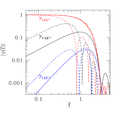
Figure 3: Overlap reduction functions for the unpolarized $I$ and circularly polarized $V$ modes for parameters $\omega=0.5$ and $\alpha=0$. The long-dashed curve is result with $d=0$ (traditional choice) for which we have $\gamma_{V,AE^{\prime}*}=\gamma_{I,AE^{\prime}*}=0$. The solid curves are for $d=1$, and the short-dashed ones are for $d=5$. The functions $|\gamma_{I,AA^{\prime}*}|$ approach 1 at ${\hat{f}}\to 0$, while the functions $\gamma_{V,AE^{\prime}*}$ and $\gamma_{I,AE^{\prime}*}$ have asymptotic behaviors $O({\hat{f}}^{1})$ and $O({\hat{f}}^{2})$ respectively. For $\alpha=0$ we have $\gamma_{I,AE^{\prime}*}=0$ (within numerical errors) at $\omega=0$.

III correlation analysis

We are now in a position to discuss how well we can estimate the monopole $V_{00}$ of circular polarization of stochastic gravitational wave background. We suppose that noises of relevant data streams $\left\{A,E,A^{\prime},E^{\prime}\right\}$ are not correlated and have identical spectrum $S(f)$ (as usually assumed for BBO). Then the signal to noise ratio (SNR) for detecting $I_{00}$ with using the combination $AA^{\prime*}$ is written as Flanagan:1993ix

$$SNR_{I}^{2}=2\left(\frac{3H_{0}^{2}}{10\pi^{2}}\right)^{2}\int_{0}^{T_{obs}}dt\int_{0}^{\infty}df\frac{|\gamma_{I,AA^{\prime*}}(f,t)|^{2}\Omega_{GW}(f)^{2}}{f^{6}S(f)^{2}},$$ (10)

where we have used the familiar quantity $\Omega_{GW}(f)\equiv{4\pi^{3/2}f^{3}I_{00}(f)}/{3H_{0}^{2}}$ ($H_{0}$: Hubble parameter) and $T_{obs}$ is the observational time. We also assumed that the amplitude of the background is much weaker than the detector noise. This corresponds to a situation when the correlation technique is effective. The signal to noise ratio $SNR_{V}$ for the target $V_{00}$ with using the combination $AE^{\prime*}$ is given by replacing the simple amplitude $\Omega_{GW}(f)$ in eq.(10) with the polarized one $\Pi\Omega_{GW}(f)$. Here the parameter $\Pi\equiv V_{00}(f)/I_{00}(f)$ is the polarization degree and we neglect its frequency dependence in this paper.

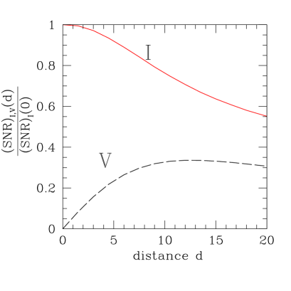
Figure 4: The signal to noise ratios for detecting $I_{00}$ and $V_{00}$ from combinations $\left\langle AA^{\prime*}\right\rangle$ and $\left\langle AE^{\prime*}\right\rangle$. The results are normalized with $SNR_{I}(0)$ for the simple orbital choice $d=0$. The shape of BBO noise curve is used and a flat spectrum $\Omega_{GW}=const$ is assumed. The polarization degree $\Pi$ is set at $\Pi=1$ for $SNR_{V}(d)$.

The overlap functions $\gamma_{\left\{I,V\right\},C}(f,t)$ depend on time $t$ through the change of the relative position between B1 and B2 as shown in figure 1. With the designed noise spectrum $S(f)$ for BBO, we numerically evaluate the integrals for $SNR_{I}$ and $SNR_{V}$ (with $\Pi=1$) as a function of the maximum separation $d\equiv D/L$ between B1 and B2. We take the observational time $T_{obs}$ as a natural number in units of the orbital period $T_{orb}$, and assumed a flat spectrum $\Omega_{GW}(f)=const$. In figure 4 ratios $SNR_{I}(d)/SNR_{I}(0)$ and $SNR_{V}(d)/SNR_{I}(0)$ are shown and these are our central results. Since we have two relevant sets $\left\{AA^{\prime*},EE^{\prime*}\right\}$ and $\left\{AE^{\prime*},EA^{\prime*}\right\}$ for measuring $I_{00}$ and $V_{00}$ respectively, these ratios can be effectively read as the results for the total network formed by B1 and B2. When we increase the distance $d$, the sensitivity for the intensity $I_{00}$ decreases monotonically due to reduction of the overlap functions $\gamma_{I,AA^{\prime*}}$ as seen in figure 3, but the sensitivity for circular polarization increases for separation $d$ up to $\sim 12$. If we take $d=5$, the ratios are $SNR_{I}(5)/SNR_{I}(0)=0.93$ and $SNR_{V}(5)/SNR_{I}(0)=0.24$. This means that the detection limit for the intensity $\Omega_{GW}$ becomes slightly ($\sim 10\%$) worse compared with the simple conventional choice at $d=0$, but we can get essentially new “sensitivity” to investigate circular polarization of gravitational wave background. For a background with a flat spectrum at $\Omega_{GW}=10^{-15}$, BBO with $d=0$ has potential to detect it at $SNR_{I}(0)=251$ by 10yr observation Seto:2005qy ; note . In other words its detection limit is written as $\Omega_{GW,lim}=2\times 10^{-17}(SNR_{I}/5)(T_{obs}/10{\rm yr})^{-1/2}$. If we take $d=5$ in stead of $d=0$, the limit becomes $\Omega_{GW,lim}=2.2\times 10^{-17}(SNR_{I}/5)(T_{obs}/10{\rm yr})^{-1/2}$ and we have the detection limit for circular polarization degree at $\Pi_{lim}=0.08(\Omega_{GW}/10^{-15})^{-1}(SNR_{V}/5)(T_{obs}/10{\rm yr})^{-1/2}$.

The author would like to thank A. Taruya and T. Tanaka for comments, and A. Cooray for various supports. This work was funded by McCue Fund at the Center for Cosmology, UC Irvine.

References

- (1) M. Maggiore, Phys. Rept. 331, 283 (2000); B. Allen, arXiv:gr-qc/9604033; C. J. Hogan, arXiv:astro-ph/0608567.
- (2) P. L. Bender et al. LISA Pre-Phase A Report, Second edition, July 1998.
- (3) E. S. Phinney et al. The Big Bang Observer, NASA Mission Concept Study (2003).
- (4) N. Seto, S. Kawamura and T. Nakamura, Phys. Rev. Lett. 87, 221103 (2001); S. Kawamura et al. Class. Quant. Grav. 23, 125 (2006).
- (5) A. Lue, L. M. Wang and M. Kamionkowski, Phys. Rev. Lett. 83, 1506 (1999).
- (6) N. Seto, “Prospects for direct detection of circular polarization of arXiv:astro-ph/0609504.
- (7) E. E. Flanagan, Phys. Rev. D 48, 2389 (1993); B. Allen and J. D. Romano, Phys. Rev. D 59, 102001 (1999).
- (8) T . A. Prince, et al, Phys. Rev. D 66, 122002 (2002).
- (9) N. Seto, Phys. Rev. D 73, 063001 (2006).
- (10) V. Corbin and N. J. Cornish, Class. Quant. Grav. 23, 2435 (2006); H. Kudoh et al. Phys. Rev. D 73, 064006 (2006).
- (11) H. Kudoh and A. Taruya, Phys. Rev. D 71, 024025 (2005).
- (12) N. Seto, Phys. Rev. D 66, 122001 (2002); Phys. Rev. D 69, 022002 (2004); N. J. Cornish and L. J. Rubbo, Phys. Rev. D 67, 022001 (2003).
- (13) N. Seto and A. Cooray, Phys. Rev. D 70, 123005 (2004); A. Taruya, arXiv:gr-qc/0607080.
- (14) This value is obtained with using parameters given in [3] for specification of BBO. We should keep in mind that they do not always represent its most up to date designed sensitivity.