The impact of correlated noise on SuperWASP detection rates for transiting extra-solar planets

Abstract

We present a model of the stellar populations in the fields observed by one of the SuperWASP-N cameras in the 2004 observing season. We use the Besançon Galactic model to define the range of stellar types and metallicities present, and populate these objects with transiting extra-solar planets using the metallicity relation of Fischer & Valenti (2005).

We investigate the ability of SuperWASP to detect these planets in the presence of realistic levels of correlated systematic noise (‘red noise’). We find that the number of planets that transit with a signal-to-noise ratio of 10 or more increases linearly with the number of nights of observations. Based on a simulation of detection rates across 20 fields observed by one camera, we predict that a total of $18.6\pm 8.0$ planets should be detectable from the SuperWASP-N 2004 data alone. The best way to limit the impact of co-variant noise and increase the number of detectable planets is to boost the signal-to-noise ratio, by increasing the number of observed transits for each candidate transiting planet. This requires the observing baseline to be increased, by spending a second observing season monitoring the same fields.

1 Introduction

Since the discovery of 51 Peg b by Mayor & Queloz (1995), a total of 181 extra-solar planets around 155 stars (as at 2006 May) have been discovered, almost exclusively by radial velocity measurements. It was only with the discovery that HD209458b transits its host star (Charbonneau et al., 2000) that both the mass and radius of an extra-solar planet were first determined. A further eight transiting extra-solar planets have been discovered in the last few years. Most of these planets have been discovered with the OGLE transit survey (e.g. Konacki et al. 2003), which is a deep-field survey. SuperWASP (Wide Angle Search for Planets) is a wide-field transit survey, which is capable of detecting planetary transits of stars that are bright enough for high precision radial velocity follow-up observations.

Transit surveys have the potential to find numerous hot Jupiter-like planets (HJs), that is Jupiter-sized planets which orbit close to their host star with periods of just a few days. The probability that a HJ system is aligned such that transits will occur is about 0.1; which is much more favourable than planets orbiting at greater distances (for an Earth-like orbit, the probability of transit alignment is 0.0046).

Crucially, the detection of transiting planets allows the determination of the average density of the planet. This is of interest for planet formation models, particularly since HD209458b appears to have an anomalously low density (Charbonneau et al., 2000), which is not well understood.

Previous attempts have been made to estimate the expected detection rates of transiting HJs by shallow, wide-field transit surveys similar to SuperWASP (e.g. Brown 2003). Based on an observing pattern consisting of 38 nights of observations spread over 91 days and a requirement that three or more transits are observed, Brown calculated the detection rate of HJs producing a transit of depth 1 per cent or greater to be 0.39 per $10^{4}$ stars. Brown also estimates that, for the same observing window function, 4.51 false alarms will be detected per $10^{4}$ stars – indicating that only eight per cent of transit signals detected will be produced by planets. These planetary transit ‘impostors’ are grazing eclipsing binaries and eclipsing binaries diluted by light from a third star (either a field star or the third member of a triple system).

The SuperWASP survey has the potential to define the population of extra-solar planets which transit nearby bright stars ($V<13$). In order for the results of SuperWASP to be properly interpreted, it is essential that the selection effects that operate in the survey are well understood. In this work, we use the findings of Pont (2006) and Pont, Zucker & Queloz (2006) to estimate SuperWASP’s detection rate in the presence of realistic levels of systematic red noise. We find that in order to detect a significant number of transiting planets, the existence of red noise necessitates much longer observing baselines than previously thought.

2 Observations

SuperWASP is a wide-field transit survey with instruments at the Isaac Newton Group on La Palma (SuperWASP-N) and at the South African Astronomical Observatory, near Sutherland, RSA (SuperWASP-S). SuperWASP-N starting observing in 2004 and SuperWASP-S was commissioned in early 2006.

Each SuperWASP installation comprises an array of eight 200mm f/1.8 Canon camera lenses, each with a four mega-pixel CCD recording a 7.8° by 7.8° field. These eight cameras are mounted on a fork mount, which is housed in an enclosure with a hydraulically operated roof. The enclosure also contains the operating computers and a weather station.

The observing strategy for the 2004 season was designed to maximise the number of stars that could be hunted for transits – overcrowded fields near the galactic plane were avoided (Christian et al., 2005). Up to eight sets of fields were observed at a time, with around a minute spent on each, including a 30 s exposure, 4 s of read-out time, and slewing, giving measurements about 7 - 8 minutes apart.

3 Data Reduction

Since each SuperWASP exposure generates an 8.4 Mb FITS file, a large quantity of data is stored and processed; this is done using a custom-written data reduction pipeline (Pollacco et al., 2006). The pipeline uses the Tycho 2 (Høg et al., 2000) and USNO B (Monet et al., 2003) catalogues to prepare an astrometric solution for each field. Aperture photometry is performed on all objects, using three different sized apertures and a blending index is assigned for each object. Airmass and CCD position trends are removed from the data before it is archived at the University of Leicester.

We search for transits in the data using a hybrid Box Least-Squares and Newton-Raphson algorithm, Hunter, developed by Collier Cameron et al. (2006). Prior to searching for transits with Hunter, the SysRem algorithm of Tamuz et al. (2005) is applied to the data to reduce systematic errors. Four components of systematic error are removed with SysRem; it is thought that two of these are caused by airmass variations and thermal changes in the camera focus, but the causes of the other two are unknown (Collier Cameron et al., 2006).

Hunter searches a grid of transit periods and epochs to fit a transit model to the data. The $\chi^{2}$ statistic is used to determine whether a best-fitting model includes a transit and, if so, to determine the best-fitting transit parameters for each candidate.

4 ‘Colours’ of noise in photometric data

Pont (2006) demonstrated that there is likely to be significant co-variance structure in the noise in data from ground-based photometric surveys, such as SuperWASP. Previous forecasts of the planet ‘catch’ from such instruments (e.g. Horne 2001) have assumed that such noise is un-correlated or ‘white’ in nature. Pont suggests that the reduced signal-to-noise caused by correlated or ‘red’ noise can account for an observed shortfall in transiting planet detections.

Noise consisting of white, independent, random noise combined with red, co-variant, systematic noise is termed ‘pink’, and, unlike white noise, cannot be removed by averaging the data. Pont showed that systematic noise, correlated on time scales equivalent to a typical hot Jupiter transit ($\approx 2.5$ hours) cannot be ignored and indeed tends to be the dominant type of noise for bright stars. It therefore seems likely that the noise in SuperWASP data will be pink.

5 Characterisation of SuperWASP noise

The simplest method of establishing the level of correlated noise present in the data is to compute a running average of the data over the $n$ data points contained in a transit-length time interval (Pont et al., 2006). The transit duration chosen here is 2.5 hours, which is the transit duration corresponding to a planet orbiting a solar analogue, with a period of 2.6 days – typical of a hot Jupiter. Since exposures are taken at roughly 7 minute intervals, there are about $n=20$ points in each interval.

If the noise is purely random, the RMS scatter in the average of $n$ data points should be $\sigma_{\mathrm{w}}=\sigma\sqrt{n}$, where $\sigma$ is the standard RMS of the whole lightcurve. If, however, there is a systematic component in the noise, the RMS scatter of the average of $n$ points will be greater than this.

The RMS scatter, $\sigma$, is calculated for each of the 822 stars determined to be non-variable in the field centred at 15h17min RA, +23°26′ dec for which lightcurves have been produced by the SuperWASP data reduction pipeline. The noisiest 25 per cent of the data points in each lightcurve, corresponding to measurements made around full moon and during Sahara dust events, are excluded from the analysis. Stars are determined to be variable, and excluded from the analysis, if $\sqrt{\sigma_{\mathrm{s}}^{2}}>0.005~{}\mathrm{mag}$, where $\sigma_{\mathrm{s}}^{2}$ is the variance caused by intrinsic stellar variability, derived from the $\chi^{2}$ statistic for a constant-flux model.

The running average, $\sigma_{\mathrm{r}}$, over 20 points is also calculated for each of these stars, with the same exclusions of the noisiest data and intrinsically variable stars.

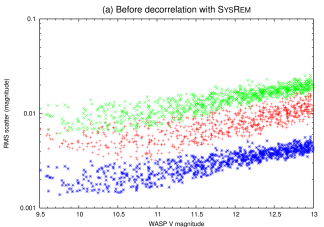
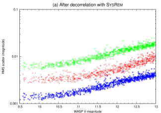
Figure 1: RMS scatter versus magnitude for non-variable stars in the field centred at 15h17min RA, +23°26′ dec both prior to (a), and after (b) decorrelation with SysRem. The upper curve shows the RMS scatter of the lightcurve of each object, $\sigma$. The middle curve shows the scatter, $\sigma_{\mathrm{r}}$, after a moving average over a 2.5 hour time interval (20 data points) was calculated. The lower curve shows the RMS scatter divided by 20, $\sigma_{\mathrm{w}}$.

Both $\sigma_{\mathrm{w}}$ and $\sigma_{\mathrm{r}}$ are calculated prior to, and after, de-correlation with SysRem. These quantities, and $\sigma$, are plotted against magnitude for the 822 non-variable stars in the field in Fig.1.

As indicated by the differences between Figs. 1 and 1, the SysRem algorithm is highly effective at reducing the levels of systematic noise present in the data. Fig. 1 also shows, however, that not all correlation in the noise is removed by SysRem. If that were the case, the $\sigma_{\mathrm{r}}$ curve would lie over the $\sigma_{\mathrm{w}}$ curve. Instead, the $\sigma_{\mathrm{r}}$ curve lies higher than $\sigma_{\mathrm{w}}$, and flattens out at about 3 mmag for bright ($V$=9.5) stars, indicating that systematic trends of this magnitude are present in the data on a 2.5 hour timescale.

6 Simulated planet catch

We model the objects in the 36 fields viewed by one of the SuperWASP cameras in the 2004 season, by using the Besançon model of the Galaxy (Robin et al., 2003) to generate a star catalogue of stars with $9.5<V<13.0$ for each of the fields. Planets are then assigned to stars that are of spectral class F, G or K and luminosity class IV or V on the basis of their metallicity, using the planet-metallicity relation of Fischer & Valenti (2005):

$$\mathcal{P}(\mathrm{planet})=0.03\times 10^{2.0[\mathrm{Fe/H}]}$$ (1)

where $\mathcal{P}(\mathrm{planet})$ is the probability that a particular star of metallicity [Fe/H] is host to a planet. The above equation is used for stars which have metallicities in the range -0.5$<$[Fe/H]$<$0.5. For stars with [Fe/H]$<-0.5$, $\mathcal{P}(\mathrm{planet})=~{}0.003$, and for [Fe/H]$>0.5$, $\mathcal{P}(\mathrm{planet})=0.3$.

Only stars of spectral type F,G and K are allocated a non-zero planet hosting probability, since the Fischer & Valenti (2005) equation is based upon radial velocity observations of stars of this type only. This does not pose a significant problem, however, as early-type stars are not numerous and have radii that are too great for transit detection. M-type stars are not particularly numerous in the Besançon-generated catalogues either (about 2.8 per cent of the stars are of type M or later), because the sample is limited by apparent magnitude, not volume. Although the transit signal produced by a Jupiter-like planet orbiting an M dwarf star will be greater than that produced by, say, a G dwarf star, M dwarfs are thought to be less likely to harbour giant planets (Adams et al., 2005). Similarly, only subgiants and dwarfs are considered planet hosts, since any planet orbiting a giant star would produce an insufficiently deep transit signature to be detected.

The probability that a star hosts a transiting planet is calculated using

$$\mathcal{P}(\mathrm{transit})=\mathcal{P}(\mathrm{planet})\times\mathcal{P}(\mathrm{alignment})$$ (2)

where $\mathcal{P}(\mathrm{alignment})$ is the probability of a given planetary system being aligned with respect to the line of sight such that a transit can be observed. This is given by

$$\mathcal{P}(\mathrm{alignment})=\mathrm{arctan}\left(\frac{\hbox{$R_{*}$\,}+\hbox{$R_{\mathrm{p}}$\,}}{a}\right)\approx\mathrm{arctan}\left(\frac{\hbox{$R_{*}$\,}}{a}\right)$$ (3)

where $R_{*}$  is the stellar radius, $R_{\mathrm{p}}$  the planetary radius and $a$ the semi-major axis of the system. The semi-major axis of each potential planetary system in the model is drawn randomly from a distribution that is uniform in log ($a$), between $0.02<a<5.25$ au.

This simple log-flat distribution of semi-major axes is compared to the actual distribution of $a$ amongst extra-solar planets discovered by Doppler surveys in Fig. 2. Our distribution appears to be a poor fit to the observed distribution in the regime favoured by transit surveys ($a\la 0.05$ au), which may lead to an overestimation of the number of very short-period planets. The distributions, however, closely agree on the fraction of planets with $a\leq$ 0.05 au - 14 per cent of the Doppler survey planets have $a\leq$ 0.05 au, while the model distribution gives 16 per cent.

Figure 2: Cumulative distribution function of extra-solar planetary semi-major axis. The filled circles represent the 186 planets discovered by radial velocity means, as at 2006 September 15. The solid line is the distribution (uniform in log ($a$) for $0.02~{}<~{}a~{}<~{}5.25$ au) used in our model.

On the basis of the probability $\mathcal{P}(\mathrm{transit})$, for each star, it is determined whether or not a star hosts a transiting planet. It is assumed, for simplicity, that all planets have a radius, $R_{\mathrm{p}}$ , equal to that of Jupiter, $R_{\mathrm{J}}$ . The depth of transit, $\Delta m$, is determined from the equation of Tingley & Sackett (2005),

$$\Delta m\approx 1.3\left(\frac{\hbox{$R_{\mathrm{p}}$\,}}{\hbox{$R_{*}$\,}}\right)^{2}$$ (4)

The factor of 1.3 in the above equation takes account of the effect of stellar limb-darkening, and although this assumes a central transit, off-centre transits will only have a slightly smaller limb-darkening factor (Tingley & Sackett, 2005).

A total of 355,429 stars are generated by the Besançon model in the 36 fields, 165586 (46.6 per cent) of which are of type F,G or K and class IV or V. The simulation described above results in the allocation of a transiting planet to 329 of these stars, although this number changes each time the simulation is run because it relies on random numbers (see §7.2 for discussion of this). The transit depths of these 329 systems are calculated using equation 4.

The detection thresholds for planet detection are determined by fitting lines to the white and red noise curves of Fig. 1. The data is modelled with a constant term and a term which is inversely proportional to the flux of each object. This leads to fitted lines of the form $\sigma~{}=~{}c_{1}~{}+~{}c_{2}~{}\left(10^{0.4V}\right)$, where $c_{1}$ and $c_{2}$ are constants which are fitted for, and $V$ is the $V$-band magnitude. The values of the constants $c_{1}$ and $c_{2}$, as determined by $\chi^{2}$ minimisation, for red and white noise are shown in Table 1.

Table 1: Fitted parameters for RMS scatter as a function of magnitude for the white and red noise cases

	$c_{1}$	$c_{2}$
$\sigma_{\mathrm{w}}$	$1.40\times 10^{-3}$	$1.96\times 10^{-8}$
$\sigma_{\mathrm{r}}$	$2.88\times 10^{-3}$	$4.34\times 10^{-8}$

All variables are defined in the text.

These functions, $\sigma_{\mathrm{w}}$ and $\sigma_{\mathrm{r}}$, of magnitude are the 1-$\sigma$ detection thresholds for the white and red noise cases respectively. The transit depths of the 329 simulated transiting planets are plotted as a function of magnitude along with the 5-$\sigma$ detection thresholds for white and red noise in Fig. 3. 28 of the 329 planets have transit depths greater than the 5-$\sigma$ detection threshold for white noise, but only one has a depth greater than the equivalent threshold when red noise is considered.

Figure 3: Transit depth versus magnitude for 329 simulated transiting extra-solar planets (points), with 5-$\sigma$ detection thresholds for red (upper curve) and white (lower curve) noise, for a single transit. If more transits are observed, the thresholds are lowered by a factor of $\sqrt{n_{\mathrm{trans}}}$. Also indicated is the stellar radius, which is directly related to the transit depth since all planets are of radius $R_{\mathrm{J}}$ .

6.1 Signal-to-noise ratios

Although Fig. 3 provides a neat illustration of the reduction in planet detection efficiency experienced when red noise is present in the data, an analysis of the signal-to-noise ratio allows a fuller picture of the red noise problem to emerge.

The signal-to-noise ratio, $S_{\rm red}$, is a function of the number of observations made in-transit, as well as the depth of the transit. In the presence of red noise, $S_{\rm red}$ is given by

$$S_{\rm red}=\frac{\Delta m\sqrt{n_{\mathrm{trans}}}}{\sigma_{\mathrm{r}}(V)}$$ (5)

where $n_{\mathrm{trans}}$ is the number of transits observed.

$S_{\rm red}$ is similar to the $S_{r}$ statistic of Pont et al. (2006), which also considers white noise. In the regime applicable to this work, where red noise dominates, $S_{r}$ simplifies to our expression for $S_{\rm red}$.

$S_{\rm red}$ is a criterion used in the selection of planetary transit candidates for follow-up spectroscopic observations (Collier Cameron et al., 2006); a signal-to-noise ratio of 10 or greater is required in order for an object to be considered as a viable transit candidate. This is a compromise between allowing too many false positive detections and rejecting large numbers of genuine transiting planets.

The $S_{\rm red}$ values of the simulated planets can be calculated using equation 5, since the transit depth, $\Delta m$, and the RMS scatter as a function of magnitude for red noise, $\sigma_{\mathrm{r}}(V)$, are already known. $n_{\mathrm{trans}}$ depends on the observing pattern and observing baseline used; here it is calculated for each simulated transiting planet using the observation times of three SuperWASP fields, the details of which are summarised in Table 2.

Table 2: The number of nights of observations for the three fields used in the signal-to-noise ratio analysis.

SuperWASP field ID	No. of nights
SW1143+3126	51
SW0044+2826	80
SW1743+3126	130

Each simulated planet is assigned a random epoch which is combined with the orbital period to produce an ephemeris for each simulated planet.

The transit duration, $D$, is calculated using the following relation,

$$D=\frac{\hbox{$R_{*}$\,}P}{\pi a}$$ (6)

where $P$ is the orbital period, and circular orbits are assumed. The ephemeris and the transit duration are used to determine whether the system is in or out of transit at each time of observation, and hence $n_{\mathrm{trans}}$ is calculated. Here, partially-observed transits with more than five observations are counted towards $n_{\mathrm{trans}}$. The signal-to-noise ratio for each simulated planet is calculated for each of the three different observing baselines; the results are plotted in Fig. 4.

The number of simulated transiting planets with $S_{\rm red}$ greater than or equal to 10 was also calculated for each of the 20 fields which have at least 10 nights of observations. Each of these fields has a different number of nights of observations, and this is reflected in the simulation, which was conducted 100 times to reduce the problems of small number statistics. A total of $3.72\pm 1.60$ planets were detected from a population of $151\pm 13$ transiting extra-solar planets. The detailed results of this simulation are shown in Table 3, and the detection rate for these fields is plotted as a function of the number of observing nights in Fig. 7. Also plotted in Fig. 7 are the detection rates produced by the full simulation for the case of both one and two seasons of observing. The detection rate of transiting extra-solar planets increases linearly with the number of observing nights.

7 Discussion

7.1 Red noise and the SysRem algorithm

The SysRem algorithm is employed to remove four components of systematic error by removing trends which are present in all the stars in a particular field. If the implementation of SysRem is changed so that the number of trends set for removal is increased to five or more, no change in the quality of the data is observed. Despite this, however, red noise – as demonstrated in §5 – is still present in the data. We postulate that this remaining red noise does not affect stars in all parts of the field and so it cannot be removed by SysRem. Instead, we suggest that the surviving red noise is localised and is most likely to be caused by variations in detector characteristics coupled with variations in the tracking of the mount. For instance, a particular group of stars may drift over the shadow cast on the CCD by a grain of dust on the optics, producing a regular dimming in a small number of objects.

7.2 Limitations of the Besançon-based model

The Besançon-based model used here has certain limitations; it should be noted that the simulation is based only on the observations from one of the SuperWASP-N cameras and it is assumed that none of the stars are blended. Only about two thirds of the generated planets have periods less than 5 days and, at present, Hunter only searches for planets with periods in this range. No planets, however, with $P>5$ days have $S_{\rm red}$ greater than 10, even with 130 nights of observations. This is because $n_{\mathrm{trans}}$, and therefore $S_{\rm red}$, decreases with increasing period.

The number of planets produced in the simulation is determined to an extent by random numbers and so varies if the simulation is repeated. The simulation used here produced 329 transiting planets from a total of 355,429 stars in the magnitude range $9.5<V<13.0$, which is a fairly typical number; the simulation was run 15 times and the number of transiting planets produced was found to be $343\pm 25$. Additionally, the relatively small number of planets around bright stars somewhat masks the fact that the signal to noise is a function of magnitude – bright objects tend to have better signal-to-noise ratios.

7.3 Detection efficiency

Because SuperWASP can observe only during the hours of darkness, it is impossible to detect transits of planets with certain ephemerides, for instance a planet that orbits with a period of exactly 1 day, where the transits occur at midday. For a relatively modest number of observing nights, if the number of observed transits, $n_{\mathrm{trans}}$, required to detect a planet is small (2 or 4, say), then the detection efficiency decreases with increasing period, but with spikes of reduced efficiency at certain pathological periods (Fig. 5).

Increasing the number of transits required for a detection causes the detection efficiency to drop dramatically at most periods. If one requires a larger number (6 or more) of transits for detection, then the detection efficiency is much lower, except for several pathological periods where the detection fraction is such that finding planets with that period is particularly favourable. Increasing the number of observing nights has the effect of increasing the detection efficiency at nearly all periods (Figs. 5,(c)).

A common property of many of the current SuperWASP transit candidates (e.g. Christian et al. 2006) is their large value of $n_{\mathrm{trans}}$, and that many of the periods coincide with the narrow pathological period ranges where there is a much greater chance of detecting a large number of transits. The effects of red noise can be reduced by increasing the signal-to-noise of the data by requiring that a larger number of transits $(\approx 10)$ are observed. In order to have a reasonable chance of observing this many transits, especially for planets with periods that are not pathologically favourable, longer time-base observations are required.

The $S_{\rm red}$ values of the simulated transiting planets are shown for 2 years of observations (130 nights in 2004, and an identical 130 nights 2 years later) in Fig. 6. This simulation shows that many more objects have a signal-to-noise ratio above the threshold of 10 after observing for a further season.

With this in mind, the 2006 SuperWASP-N observing season is to be dedicated to observing the same fields as in the 2004 season. A further advantage of this policy is that the candidate planets will have very well determined ephemerides, which will aid follow-up work.

Figure 4: Signal-to-noise ratio versus magnitude for 329 simulated transiting extra-solar planets, for 51, 80 and 130 nights of data. The dotted line indicates a signal-to-noise ratio of 10, the threshold used when compiling transit candidate lists.

Figure 5: Transit detection efficiency as a function of period for fields with observations on 51, 80 and 130 nights. The solid, upper curve is for the requirement that at least 2 transits are observed for a detection; the dashed, middle curve for 4 transits; and the dotted, lower curve for 6.

Figure 6: As Fig. 4, but for 2 seasons each consisting of 130 nights of data. 56 stars are above the $S_{\rm red}$ threshold of 10.

Figure 7: Detection rate (a detection is defined as $S_{\rm red}>10$) of transiting extra-solar planets versus number of nights of observations. The squares correspond to one season of observations, while the triangles represent an additional 130 nights of observations in a second season. The open circles represent the 20 fields included in Table 3.

Table 3: Simulated planetary detection rates in the twenty fields that were observed for more than ten nights by one of the SuperWASP-N cameras in 2004.

Field ID	No. of nights	No. of	No. of stars		No. of planets with	Detections
	of observations	observations	Model	Observed	$S_{\rm red}\geq 10$ in simulation	per $10^{4}$ stars
SW0043+3126	88	2962	6150	4746	$0.12\pm 0.32$	0.20
SW0044+2826	80	2851	5684	7353	$0.10\pm 0.30$	0.18
SW0143+3126	72	2251	6354	7840	$0.06\pm 0.24$	0.01
SW0243+3126	61	1646	7114	8235	$0.07\pm 0.26$	0.10
SW0343+3126	46	1286	9630	8465	$0.03\pm 0.17$	0.03
SW0443+3126	44	911	16062	8314	$0.04\pm 0.20$	0.02
SW0543+3126	38	539	21255	15021	$0.01\pm 0.10$	0.00
SW1043+3126	31	473	2939	2775	$0.01\pm 0.10$	0.03
SW1143+3126	51	813	2628	2508	$0.03\pm 0.17$	0.11
SW1243+3126	86	2157	2577	2605	$0.07\pm 0.35$	0.27
SW1342+3824	103	2578	2482	2724	$0.09\pm 0.32$	0.36
SW1443+3126	125	3618	2988	3071	$0.24\pm 0.51$	0.80
SW1543+3126	130	4422	3899	3963	$0.27\pm 0.47$	0.69
SW1643+3126	129	4795	5388	6233	$0.37\pm 0.59$	0.69
SW1739+4723	119	4401	5361	8791	$0.41\pm 0.58$	0.76
SW1743+3126	130	5214	8712	11681	$0.45\pm 0.65$	0.52
SW1745+1727	110	3590	13700	17818	$0.38\pm 0.60$	0.28
SW2143+3126	88	3672	15145	24129	$0.27\pm 0.53$	0.18
SW2243+3126	118	4388	9175	14330	$0.42\pm 0.60$	0.46
SW2343+3126	112	3629	6913	9488	$0.28\pm 0.53$	0.41
Total			154156	170090	$3.72\pm 1.60$	0.24

7.4 Comparison of detection rates with previous work

The simulation described in this paper allows comparison with the detection rate of transiting HJs estimated by Brown (2003), who takes no account of red noise. Of the planets generated in the simulation, 63 have a transit depth deeper than one per cent, resulting in about 20 detectable planets if we assume that the fraction of transits recovered is about 0.3 for the 38 nights of observations described by Brown. Since there are $\sim 3.55\times 10^{5}$ stars in our simulation, this gives a detection rate of 0.56 per $10^{4}$, which is comparable to the 0.39 per $10^{4}$ of Brown. However, our signal-to-noise ratio analysis suggests that, in reality, observations must be made for between 80 and 130 nights for the detection rate of HJs to be as high as 0.39 per $10^{4}$ stars (Fig. 7).

8 Conclusions

We conclude that there is a significant component of systematic, red noise present in data from SuperWASP-N. The SysRem algorithm of Tamuz et al. (2005) appears highly effective at reducing the level of red noise, but fails to eliminate it entirely. The remaining red noise is present in the data at a level of about 3 mmag on time-scales of 2.5 hours, roughly equivalent to a typical transit duration time. This remaining noise has a significant impact on the efficacy of planet detection, as demonstrated by a Monte Carlo simulation based on the Besançon Galaxy model.

Our analysis reveals that if observations are conducted for only 51 nights, none of the simulated transiting planets produces a transit detection with a signal-to-noise ratio of 10 or more. A total of $3.72\pm 1.60$ planets which transit with $S_{\rm red}~{}\geq~{}10$ are predicted for the fields observed in 2004 by one SuperWASP-N camera, which is representative of the other four cameras, so $18.6\pm 8.0$ planets are predicted in total. In order to improve the $S_{\rm red}$, and thus increase the number of detectable planets, a greater number of transits must be observed in the data set of a particular object. This requires observations to be made over a longer time period.

On the basis of the transit detection rates predicted here, the SuperWASP consortium have decided to continue observing all the fields that were monitored during 2004. We expect that this will enhance greatly the number of planetary transit events detected at non-pathological periods.

9 Acknowledgements

The WASP Consortium consists of representatives from the Universities of Cambridge (Wide Field Astronomy Unit), Keele, Leicester, The Open University, Queens University Belfast and St Andrews, along with the Isaac Newton Group (La Palma) and the Instituto de Astrofísica de Canarias (Tenerife). The SuperWASP cameras were constructed and are operated with funds made available from the Consortium Universities and PPARC. AMSS wishes to acknowledge the financial support of a UK PPARC studentship.

References

- Adams et al. (2005) Adams F. C., Bodenheimer P., Laughlin G., 2005, Astronomische Nachrichten, 326, 913
- Brown (2003) Brown T. M., 2003, ApJ, 593, L125
- Charbonneau et al. (2000) Charbonneau D., Brown T. M., Latham D. W., Mayor M., 2000, ApJ, 529, L45
- Christian et al. (2006) Christian D., Pollacco D., Skillen I., Street R., Keenan F., Clarkson W., Collier-Cameron A., Kane S., Lister T., West R., Enoch R., Evans N., Fitzsimmons A., Haswell C., Hellier C., Hodgkin S., Horne K., 2006, MNRAS, in press, astro-ph/0608142
- Christian et al. (2005) Christian D., Pollacco D. L., Clarkson W. I., Collier-Cameron A., Evans N., Fitzsimmons A., Haswell C. A., Hellier C., Hodgkin S. T., Horne K. D., Kane S. R., Keenan F. P., Lister T. A., Norton A. J., Ryans R., Skillen I., Street R. A., West R. G., Wheatley P. J., 2005, in 13th Cambridge Workshop on Cool Stars, Stellar Systems and the Sun Current status of the SuperWASP project. ESA SP-560, pp 475–477
- Collier Cameron et al. (2006) Collier Cameron A., Pollacco D., Street R. A., Lister T. A., West R. G., Wilson D. M., Pont F., Christian D., Clarkson W. I., Evans A., Haswell C. A., Hellier C., Hodgkin S. T., Horne K., Irwin J., Kane S., Norton A., Skillen I., Wheatley P., 2006, MNRAS, submitted, astro-ph/0609418
- Fischer & Valenti (2005) Fischer D. A., Valenti J., 2005, ApJ, 622, 1102
- Høg et al. (2000) Høg E., Fabricius C., Makarov V. V., Urban S., Corbin T., Wycoff G., Bastian U., Schwekendiek P., Wicenec A., 2000, A&A, 355, L27
- Horne (2001) Horne K., 2001, in Dent W. R. F., ed., Techniques for the detection of planets and life beyond the solar system, 4th Annual ROE Workshop, held at Royal Observatory Edinburgh, Scotland, Nov 7-8, 2001. Edited by W.R.F. Dent. Edinburgh, Scotland: Royal Observatory, 2001, p.5 Planetary Transit Searches: Hot Jupiters Galore. pp 5–+
- Konacki et al. (2003) Konacki M., Torres G., Jha S., Sasselov D. D., 2003, Nat, 421, 507
- Mayor & Queloz (1995) Mayor M., Queloz D., 1995, Nat, 378, 355
- Monet et al. (2003) Monet D. G., Levine S. E., Canzian B., Ables H. D., Bird A. R., Dahn C. C., Guetter H. H., Harris H. C., Henden A. A., Leggett S. K., Levison H. F., Luginbuhl C. B., Martini J., Monet A. K. B., Munn J. A., Pier J. R., Rhodes A. R., Riepe B., 2003, AJ, 125, 984
- Pollacco et al. (2006) Pollacco D., Skillen I., Collier Cameron A., Christian D., Hellier C., Irwin J., Lister T., Street R., West R., Anderson D., Clarkson W., Deeg H., B. E., A. E., Fitzsimmons A., Haswell C., Hodgkin S., Horne K., Kane S., Keenan F., Maxted P., Norton A., Osborne J., 2006, PASP, in press, astro-ph/0608454
- Pont (2006) Pont F., 2006, in Arnold L., Bouchy F., Moutou C., eds, Tenth Anniversary of 51 Peg-b: Status of and prospects for hot Jupiter studies Photometric searches for transiting planets: results and challenges. pp 153–164
- Pont et al. (2006) Pont F., Zucker S., Queloz D., 2006, MNRAS, in press, astro-ph/0608597
- Robin et al. (2003) Robin A. C., Reylé C., Derrière S., Picaud S., 2003, A&A, 409, 523
- Tamuz et al. (2005) Tamuz O., Mazeh T., Zucker S., 2005, MNRAS, 356, 1466
- Tingley & Sackett (2005) Tingley B., Sackett P. D., 2005, ApJ, 627, 1011