Simulation of Cosmic Ray $\nu$ Interactions in Water

Abstract

The program CORSIKA, usually used to simulate extensive cosmic ray air showers, has been adapted to a water medium in order to study the acoustic detection of ultra high energy neutrinos. Showers in water from incident protons and from neutrinos have been generated and their properties are described. The results obtained from CORSIKA are compared to those from other available simulation programs such as Geant4.

1 Adaptation of the CORSIKA program to a water medium

The air shower program, CORSIKA (version 6204) [1], has been adapted to run in sea water i.e. a medium of constant density of 1.025 g per cm³ rather than the variable density needed for an air atmosphere. Sea water was assumed to consist of a medium in which $66.2\%$ of the atoms are hydrogen, $33.1\%$ of the atoms are oxygen and $0.7\%$ of the atoms are made of common salt, NaCl. The salt was assumed to be a material with atomic weight and atomic number A=29.2 and Z=14, the mean of sodium and chlorine. The purpose of this is to maintain the structure of the program as closely as possible to the air shower version which had two principal atmospheric components (oxygen and nitrogen) with a trace of argon. The presence of the salt component had an almost undetectable effect on the behaviour of the showers.

Other changes made to the program to accomodate the water medium include a modification of the stopping power formula to allow for the density effect in water. This only affects the energy loss in hadrons since the stopping powers for electrons are part of the EGS [2] package which is used by CORSIKA to simulate the propagation of the electromagnetic component of the shower. Smaller radial binning of the shower was also required since shower radii in water are much smaller than those in air. In addition the threshold for the LPM effect [3], which suppresses pair production from photons and bremsstrahlung from electrons at high energy, was reduced to the much lower value necessary for water. Similarly, the interactions of $\pi^{0}$s had to be simulated at lower energy than in air because of the higher density water medium. In all about 100 detailed changes needed to be made to the CORSIKA program to accomodate the water medium.

To test the implementation of the LPM effect [3] in the program 100 showers from incident gamma ray photons were generated and the mean depth of the first interaction (the mean free path) calculated. The observed mean free path was found to be in agreement with the expected behaviour when both the suppression of pair production and photonuclear interactions were taken into account (see figure 1). This showed that the LPM effect had been properly implemented in CORSIKA.

Considerable fluctuations between showers occurred giving the following observed values of the ratios of the root mean square deviations to the mean value in proton showers: rms peak energy deposit to the peak energy deposit was observed to be $14\%$ at $10^{5}$ GeV reducing to $4\%$ $10^{11}$ GeV, that for the depth of the peak position varied from $19\%$ to $7.4\%$ and for the shower width from $63\%$ to $18\%$. To smooth out such fluctuations averages of 100 generated showers will be taken in the following. The statistical error on the averages is then given by these RMS values divided by $\sqrt{1}00$. The hadronic energy contributes only about 10$\%$ to the shower energy at the shower peak, the remainder being carried by the electromagnetic part of the shower. This is a well known effect in calorimeters.

2 Comparison with Other Simulations

2.1 Comparison with Geant4

Proton showers were generated in sea water using the program Geant4 (version 8) [4] and compared with those generated in CORSIKA. Unfortunately, the range of validity of Geant4 physics models for hadronic interactions does not extend beyond an energy of $10^{5}$ GeV. Hence the comparison is restricted to energies below this.

Figs. 2 show the longitudinal distributions of proton showers at energies of $10^{4}$ and $10^{5}$ GeV (averaged over 100 showers) as determined from Geant4 and CORSIKA. The showers from CORSIKA tend to be slightly broader and with a smaller peak energy than those generated by Geant4. The difference in the peak height is $\sim 5\%$ at $10^{4}$ GeV rising to $\sim 10\%$ at energy $10^{5}$ GeV. Figs. 3 show the radial distributions. The differences in the longitudinal distributions are reflected in the radial distributions. However, the shapes of the radial distributions are very similar between Geant4 and CORSIKA. CORSIKA produces somewhat less ($\sim 20\%$) energy than Geant4 near the shower axis at depths between 450 and 850 g cm^-2 where most of the energy is deposited. The acoustic signal from a shower is most sensitive to the distribution near the axis ($r\sim 0$).

2.2 Comparison with Alvarez-Muniz and Zas Simulation

The CORSIKA simulation was also compared with the longitudinal shower profile computed in the simulation by Alvarez-Muniz and Zas [5]. There was a reasonable agreement between the longitudinal shower shapes from CORSIKA and those shown in fig. 2 of ref. [5]. However, the number of electrons at the peak of the CORSIKA showers was $\sim 20\%$ lower than those from ref. [5]. Their procedure involves a fast hybrid Monte Carlo which simulates one dimensional showers down to a cross over energy below which parameterisations are used. The total number of electrons produced is sensitive to the lower energy down to which the simulation proceeds, which is not specified in the paper. Given this unknown, the agreement between CORSIKA and the simulation of ref. [5] is probably satisfactory.

3 Comparison of Radial Distributions and Published Parameterisations

Niess and Bertin [6, 7] parameterise the radial density distribution of showers in water as

$$\rho(r)=kx^{n}$$ (1)

where $k$ is a normalising constant chosen arbitrarily here at each depth, $x=3.5/r$ and $n=1.66-0.29z/z_{max}$ for $r<3.5$ cm or $n=2.7$ for $r>3.5$ cm. This is the parameterisation for pion showers given in [7]. Here $z$ is the depth and $z_{max}$ is the depth of maximum energy deposition. The energy deposited per cm at radius $r$ is then proportional to $r\rho(r)$. Fig 4 shows the radial distribution from CORSIKA compared with this parameterisation. There is reasonable agreement between them particularly at small values of $r$. Hence the two should predict similar distributions of the frequencies of acoustic signals from the hadron shower in water.

The SAUND Collaboration [8] uses the following parameterisation [9] for the energy deposited per unit depth, $z$, and per unit annular thickness at radius $r$ from a shower of energy $E$

$$\frac{d^{2}E}{drdz}=Ek(\frac{z}{z_{max}})^{t}\exp{(t-z/\lambda)}~{}2\pi r\rho(r)$$ (2)

where $z_{max}=0.9X_{0}\ln(E/E_{c})$ is the maximum shower depth, $X_{0}=36.1$ g cm^-2 is the radiation length and $E_{c}=0.0838$ GeV is the critical energy in water. The constants $t=z_{max}/\lambda$ where $\lambda=130-5\log_{10}(E/10^{4}\mathrm{GeV})$ g cm^-2 and $k=t^{t-1}/\exp{(t)}\lambda\Gamma(t)$. The radial density is given by

$$\rho(r)=\frac{1}{r_{M}^{2}}a^{s-2}(1+a)^{s-4.5}\frac{\Gamma(4.5-s)}{2\pi\Gamma(s)\Gamma(4.5-s)}$$ (3)

where $a=r/r_{M}$ with $r_{M}=9.04$ g cm^-2 the Moliere radius in water and $s=1.25$. Fig 5 shows the radial distributions from CORSIKA compared with the absolute predictions of this parameterisation. There is qualitative agreement between them. However, CORSIKA predicts relatively more energy at small $r$ i.e. a harder frequency spectrum for acoustic signals.

4 Simulation of $\nu$ induced Showers

The CORSIKA program has an option to simulate the interactions of neutrinos at a fixed point [10]. The first interaction is generated by the HERWIG package [11]. Some problems have been encountered in simulating $\nu$ showers at energies above $4~{}10^{7}$ GeV. However, the package seems to work well at energies below this. At these energies the mean value of the energy transfered to the hadrons in the interaction is about $25\%$ of the incident neutrino energy [12] and this fluctuates in different interactions between zero and $100\%$ with an RMS value of $25\%$. Hence much larger fluctuations occurred for neutrino than for proton showers. The shapes of the hadron shower profiles for neutrinos were observed to be similar to those generated by proton showers in water at an energy of $25\%$ of the neutrino energy.

5 Conclusions

The program CORSIKA has been modified to work in a water medium. Hadron and electromagnetic showers can be generated routinely. Neutrino interactions at low energy can be generated by the HERWIG package interfaced to CORSIKA and it may be possible to extend this to higher energies.

5.1 Acknowledgments

I wish to thank all my colleagues in the ACoRNE Collaboration for their help and support. Special thanks go to Jon Perkin who produced several of the plots shown in this talk. I should also like to thank Ralph Engel, Dieter Heck, Johannes Knapp and Tanguy Pierog for their assistance in modifying the CORSIKA program.

Figure 1: The interaction length for high energy gamma rays versus the photon energy measured in CORSIKA (data points with statistical errors). The dash dotted curve shows the pair production length computed from the LPM effect using the formulae of Migdal [3]. The solid curve shows the computed total interaction length, including both pair production and photonuclear interactions computed using the values of the photonuclear cross section from CORSIKA.

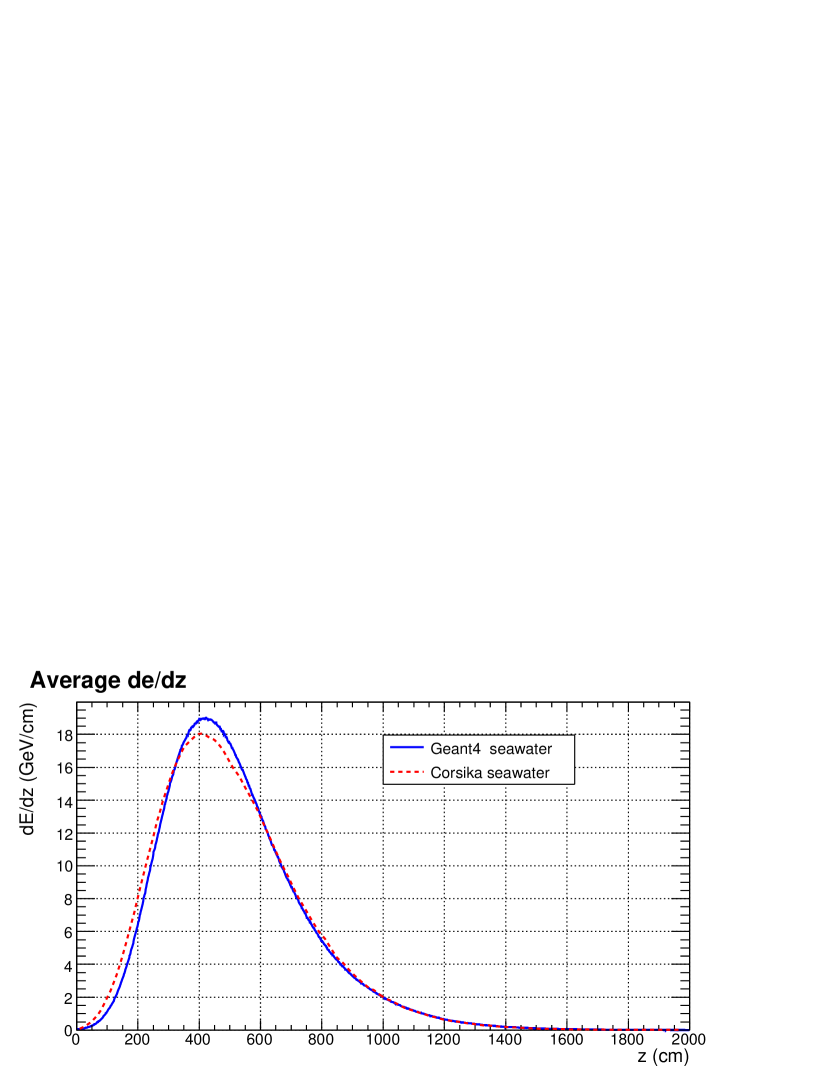
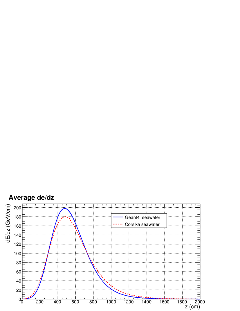
Figure 2: Averaged longitudinal energy deposited per unit path length of 100 proton showers at energy $10^{4}$ GeV (upper plot) and $10^{5}$ GeV (lower plot) generated in Geant4 and Corsika versus depth in the water.

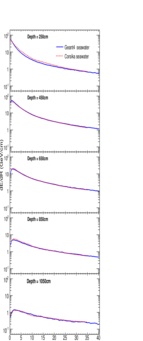
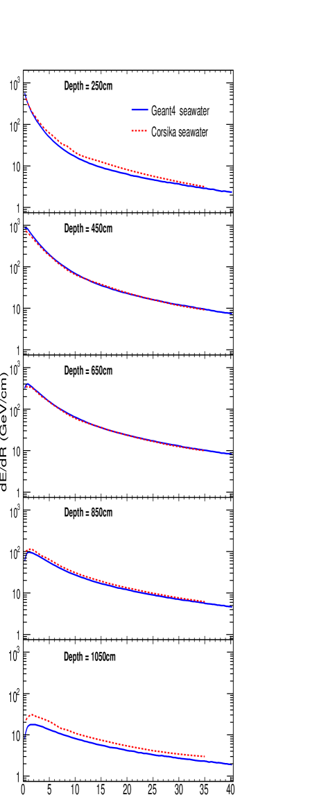
Figure 3: Averaged radial energy deposited per 20 gm cm^-2 vertical slice per unit radial distance for 100 proton showers at energy $10^{4}$ GeV (left hand plot) and $10^{5}$ GeV (right hand plot) generated in Geant4 and CORSIKA versus distance from the axis in the water for different depths of the shower.

Figure 4: Averaged radial energy deposited per 20 gm cm^-2 vertical slice per unit radial distance for 100 proton showers at energy $10^{6}$ GeV (left hand plot) and $10^{11}$ GeV (right hand plot) in water compared to the Niess-Bertin parameterisation [7].

Figure 5: Averaged radial energy deposited per 20 gm cm^-2 vertical slice per unit radial distance for 100 proton showers at at energy $10^{6}$ GeV (left hand plot) and $10^{11}$ GeV (right hand plot) in water compared to the parameterisation used by the SAUND Collaboration [9].

References

- [1] http://www-ik.fzk.de/corsika
- [2] W.R. Nelson, H. Hirayama and D.W.O. Rogers, report number SLAC-265.
-
[3]
L.D. Landau and I.J. Pomeranchuk, Dokl. Akad. Nauk. SSSR
92 (1953) 535 and 92 (1953) 735. These papers are available in
English in L. Landau, “The Collected Papers of L.D. Landau”, Pergamon Press 1965.
A.B. Migdal, Phys. Rev. 103 (1956) 1811. - [4] Geant4, J. Allison et al., Nucl. Inst. and Meths. in Phys. Research A506 (2003) 250 and IEEE Transactions on Nucl. Science 53 (2006) 270.
- [5] J. Alvarez-Muniz and E. Zas, Phys. Lett. B434 (1998) 396 (astro-ph/9806098).
- [6] V. Niess and V. Bertin astro-ph/0511617 and V. Niess, PhD Thesis, CPPM, Marseille.
- [7] V. Niess, PhD Thesis, CPPM, Marseille, see equations 1-55 and 1-56.
- [8] J. Vandenbroucke, G. Gratta, N. Lehtenin, Astrophys. J. 621 (2005) 301. (astro-ph/0406105).
- [9] J. Vandenbroucke, private communication.
- [10] O. Pisanti, private communication, see also M. Ambrosio et al., astro-ph/0302062.
- [11] HERWIG, G. Corcella et al., hep-ph/0011363.
- [12] R. Ghandi, C. Quigg, M.H. Reno, I. Sarcevic, Astroparticle Physics 5 (1996) 81.