MECI: A Method for Eclipsing Component Identification

Abstract

We describe an automated method for assigning the most probable physical parameters to the components of an eclipsing binary, using only its photometric light curve and combined colors. With traditional methods, one attempts to optimize a multi-parameter model over many iterations, so as to minimize the chi-squared value. We suggest an alternative method, where one selects pairs of coeval stars from a set of theoretical stellar models, and compares their simulated light curves and combined colors with the observations. This approach greatly reduces the parameter space over which one needs to search, and allows one to estimate the components’ masses, radii and absolute magnitudes, without spectroscopic data. We have implemented this method in an automated program using published theoretical isochrones and limb-darkening coefficients. Since it is easy to automate, this method lends itself to systematic analyses of datasets consisting of photometric time series of large numbers of stars, such as those produced by OGLE, MACHO, TrES, HAT, and many others surveys.

1 Introduction

Eclipsing double-lined spectroscopic binaries provide the only method by which both the masses and radii of stars can be estimated without having to resolve spatially the binary or rely on astrophysical assumptions. Despite the large variety of models and parameter-fitting implementations [e.g. WD (Wilson & Devinney, 1971) and EBOP (Etzel, 1981; Popper & Etzel, 1981)], their underlying methodology is essentially the same. Photometric data provide the light curve of the eclipsing binary (EB), and spectroscopic data provide the radial velocities of its components. The depth and shape of the light curve eclipses constrain the components’ brightness and fractional radii, while the radial velocity sets the length scale of the system. In order to characterize fully the components of the binary, one needs to combine all of this information. Only a small fraction of all binaries eclipse, and spectra with sufficient resolution and signal-to-noise can be gathered only for bright stars. The intersection of these two groups leaves a small number of stars.

Over the past decade, the number of stars with high-quality, multi-epoch, photometric data has grown dramatically due to the growing interest in finding gravitational lensing events (Wambsganss, 2006) and eclipsing extrasolar planets (Charbonneau et al., 2006). In addition, major technical improvements in both CCD detectors and implementations of image-difference analysis techniques (Crotts, 1992; Alard et al., 1998; Alard, 2000) enable simultaneous photometric measurements of tens of thousands of stars in a single exposure. Today, there are many millions of light curves available from a variety of surveys, such as OGLE (Udalski et al., 1994), MACHO (Alcock et al., 1998), TrES (Alonso et al., 2004), HAT (Bakos et al., 2004), and XO (McCullough et al., 2006). Despite the increase in photometric data, there has not been a corresponding growth in the quantity of spectroscopic data, nor is this growth likely to occur in the near future. Thus, the number of fully-characterized EBs has not grown at a rate commensurate with the available photometric datasets.

In recent years, there has been a growing effort to mine the wealth of available photometric data, by employing automated pipelines which use simplified EB models in the absence of spectroscopic observations and hence without a fixed physical length scale and absolute luminosity (Wyithe & Wilson, 2001, 2002; Devor, 2004, 2005). In this paper, we present a method that utilizes theoretical isochrones and multi-epoch photometric observations of the binary system to estimate the physical parameters of the component stars, while still not requiring spectroscopic observations.

Our Method for Eclipsing Component Identification (MECI), finds the most probable masses, radii, and absolute magnitudes of the stars. The input for MECI is an EB’s photometric light curve and out-of-eclipse colors (we note that in the absence of color information, the accuracy in the estimation of the stellar parameters is significantly reduced; §4.2). This approach can be used to characterize quickly large numbers of eclipsing binaries; however it is not sufficient to improve stellar models, since underlying isochrones must be assumed.

In a previous paper (Devor & Charbonneau, 2005), we outlined the ideas behind both MECI and a closely related, “quick and dirty” alternative, which we called MECI-express. Though MECI-express is much faster and easier to implement, it is also far less accurate. For this reason we will not discuss it further, and instead concentrate exclusively on MECI. We discuss its applications (§2), aspects of its implementation (§3), tests of its accuracy (§4), and finally summarize our findings (§5).

2 Motivation

2.1 Characterizing the binary stellar population

First and foremost, MECI is designed as a high throughput means to systematically estimate the masses of large numbers of stars. Though the result in each system is uncertain, by statistically analyzing large catalogs, one can reduce the non-systematic errors. Much work has already been invested into characterizing binary systems through spectroscopic binary surveys (e.g. Duquennoy & Mayor, 1991; Pourbaix et al., 2004), yet the limited data and their large uncertainties have led to inconsistent results (Mazeh et al., 2005). The driving questions that have spurred debate in the community include: What are the initial mass functions of the primary and secondary components? How do they relate to the initial mass function of single stars? What is the distribution of the components’ mass ratio, $q$, and in particular, does it peak at unity? This lack of understanding is further highlighted by the fact that most of the stars in our galaxy are members of binary systems, and that these questions have lingered for over a century. MECI may help sort this out by systematically characterizing the component stars of many EB systems.

By requiring only photometric data, a survey using MECI can study considerably fainter binary systems than spectroscopic surveys, and thus remain complete to a far larger volume. As an illustrative example, the difference image analysis of the bulge fields of OGLE II, using the Las Campanas $1.3$m Warsaw telescope in a drift-scan mode (an effective exposure time of $87$ seconds), attained a median noise level of $0.1$ mag, for $I=18$ binaries, even in moderately crowded fields (Wozniak, 2000). In contrast to this, the CfA digital speedometer on the $1.5$m FLWO telescope has a spectral resolution of $R\simeq 35,000$ (at $5177$Å) and typically yields a radial velocity precision of $0.5\ {\rm km\,s^{-1}}$, with a faint magnitude limit of $V=13$ (Latham, 1992). Though the limiting magnitudes are very much dependent on the throughput of the relevant instruments and the precision one wishes to achieve, this $5$ magnitude difference for telescopes of similar aperture corresponds to a factor of $10$ in distance or $1000$ in volume, and illustrates the significant expansion that can be achieved by purely photometric surveys. Conversely, one can achieve the same magnitude limit with an aperture $10$ times smaller. The success of this approach has been demonstrated by several automated observatories, such as TrES (Alonso et al., 2004) and HAT (Bakos et al., 2004), which each use networks of observatories with 10-cm camera lenses to monitor stars to $V\simeq 13$.

2.2 Identifying low-mass main-sequence EBs

One of the most compelling applications of MECI will be to sort quickly thousands of EBs present in large photometric surveys, and to subsequently select a small subset of objects from the resulting catalog for further study. In particular, lower main-sequence stars that are partially or fully convective have not been studied with a level of detail remotely approaching that of solar-type (and more massive) stars. This is particularly troubling since late-type stars are the most common in the Galaxy, and dominate its stellar mass. It has been shown that models underestimate the radii of low-mass stars by as much as $20$% (Lacy, 1977a; Torres & Ribas, 2002), a significant discrepancy considering that for solar-type stars the agreement with the observations is typically within $1-2$% (Andersen, 1998). Similar problems exist for the effective temperatures predicted theoretically for low-mass stars. Progress in this area has been hampered by the lack of suitable M-dwarf binary systems with accurately determined stellar properties, such as mass, radius, luminosity, and surface temperature. Detached eclipsing systems are ideal for this purpose, but only five are known among M-type stars: CM Dra (Lacy, 1977b; Metcalfe et al., 1996), YY Gem (Kron, 1952; Torres & Ribas, 2002), CU Cnc (Delfosse et al., 1999; Ribas, 2003), and OGLE BW3 V38 (Maceroni & Rucinski, 1997; Maceroni & Montalbán, 2004), and TrES-Her0-07621 (Creevey et al., 2005). They range in mass from about $0.25M_{\sun}$ (CM Dra) to $0.6M_{\sun}$ (YY Gem). The number of such objects could be greatly increased by using tools such as MECI to mine the extant photometric datasets to locate these elusive low-mass systems.

2.3 EBs as standard candles

Using MECI, we are able to estimate the absolute magnitude of the binary system. Together with its extinction-corrected out-of-eclipse apparent magnitude, we can then calculate the distance modulus to any given EB. The estimation of distances to EBs dates back to Stebbing (1910), and their use as distance candles in the modern astrophysical context was recently elucidated by Paczynski (1997). However, unlike these studies, MECI does not require spectroscopy and therefore is able to analyze binaries that are significantly less luminous (see §2.1). Though the distance estimation from MECI will be uncertain, in many cases this will still be an improvement over existing methods. For example, if there are many EBs in a stellar cluster, the distance estimate can be greatly improved by combining their results, to reduce the non-systematic errors by a factor of the square root of the number of systems. Following Guinan et al. (1996), one might be able to use such clustered EB standard candles to better constrain the distance to the LMC and SMC, and thus be able to further constrain the bottom of the cosmological distance ladder. In the case of MECI, the uncertainties of each distance measurement will be considerably larger, but as suggested by Tsevi Mazeh (2005, personal communication), this will be compensated for by the far larger number of measurements that can be made. Another intriguing application of such EB standard candles is to map large scale structures in the Galaxy, such as the location and orientation of the galactic bar, arms, and merger remnants (see, for example, Vallée, 2005, and references therein).

3 Method

The EB component identification is performed in two stages. First the orbital parameters of the EB are estimated (§3.1), then the most likely stellar parameters are identified (§3.2). Our implementation of MECI has the option to fix the estimates of the orbital parameters, or to fine-tune them for each stellar pairing considered in the second stage. The average running time for MECI to analyze a $1000$-point light curve on a single $3.4$GHz Intel Xeon CPU is $0.4$ minutes. If we permit fine tuning of the orbital parameters for each pairing, the running time grows to $6$ minutes per light curve.

3.1 Stage 1: Finding the orbital parameters

In the first stage, we estimate the EB’s orbital parameters from its light curve. Many EBs have orbital periods of a few days or less, owing to the greater probability for such systems to present mutual eclipses, and to the limited baselines in the datasets from which they are identified. Most of these systems will have orbits that have been circularized due to tidal effects. For such circular orbits, the only parameters we seek are the orbital period, $P$, and epoch of periastron, $t_{0}$. For non-circular orbits we also fit the orbital eccentricity, $e$, and the argument of periastron, $\omega$. The period is determined using a periodogram, and the remaining parameters are obtained through fitting the offset, duration and time interval between the light curve’s eclipses (see below). Holding these parameters fixed at these initial estimates significantly reduces the computational requirements of MECI.

We postpone fitting the orbital inclination, $i$, until the second stage, since it is difficult to determine this parameter robustly without first assuming values for the stellar radii and masses. This difficulty arises because it is often difficult to distinguish a small secondary component from a large secondary component in a grazing orbit. In stage 2, additional information, such as the theoretical stellar mass-radius relation and colors are used to help resolve this degeneracy.

The procedure for fitting the aforementioned parameters from the EB light curve is a well-studied problem (Kopal, 1959; Wilson & Devinney, 1971; Etzel, 1991). We chose to estimate the period with a variant of the analysis of variances (AOV) periodogram by Schwarzenberg-Czerny (1989, 1996). We then use the Detached Eclipsing Binary Light curve (DEBiL) fitter by Devor (2004, 2005) for fitting the remaining orbital parameters. For non-circular systems, following Kopal (1959) and Kallrath & Milone (1999), we estimate the orbital eccentricity and argument of periastron from the orbital period, the duration of the eclipses, $\Theta_{1,2}$, and the time interval between the eclipse centers, $\Delta t$, as follows:

$$\omega \simeq \arctan\left[\frac{2}{\pi}\left(\frac{\Theta_{1}-\Theta_{2}}{\Theta_{1}+\Theta_{2}}\right)\left(\frac{\Delta t}{P}-\frac{1}{2}\right)^{-1}\right],{\rm\ and}$$ (1)

$$e \simeq \frac{\pi}{2\cos\omega}\left|\frac{\Delta t}{P}-\frac{1}{2}\right|.$$ (2)

In practice, it is difficult to accurately determine the eclipse duration. We estimate this duration by first calculating the median flux outside the eclipses, then estimating the midpoints and depths of the eclipses using a spline. We then assign the duration of each eclipse to be the time elapsed from the moment at which the light curve during ingress crosses the midpoint between the out-of-eclipse and bottom-of-eclipse fluxes, until the moment at which the light curve crosses the corresponding point during egress.

3.2 Stage 2: Finding the absolute stellar parameters

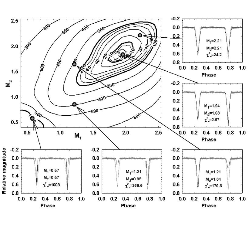
Figure 1: The large upper-left panel shows the MECI $\chi^{2}_{\nu}$ surface as a function of the assumed masses (in units of $M_{\sun}$) of the component stars in the WW Camelopardalis system. The model light curve at five locations in the grid is shown in the smaller panels, overplotted on the observed light curve from (Lacy et al., 2002). A high-quality version of this figure can be seen at: http://cfa-www.harvard.edu/$\sim$jdevor/MECI/paper/

In the second stage, we estimate the EB’s absolute stellar parameters by iterating through many possible stellar pairings, simulating their expected light curves (see Fig. 1), and finding the pairing that minimizes the $\chi^{2}_{\nu}$ function (see §3.3). The parameters we fit are the masses of the two EB components, $M_{1,2}$, their age (the components are assumed to be coeval), and their orbital inclination, $i$. Optionally, we can also fine-tune the orbital parameters obtained from the first stage. This option is necessary only for binaries with eccentric orbits, since varying their inclination will affect the fit of their previously estimated orbital parameters. The flow diagram for the entire procedure is shown in Figure 2.

If an estimate of the out-of-eclipse combined apparent magnitude, $mag_{comb}$, of the EB (i.e. the light curve plateau) is available, we may also estimate the distance modulus. If $mag_{comb}$ is not available (for example, if the light curve has been normalized), the distance modulus cannot be evaluated unless an independent measurement of the out-of-eclipse brightness is available. In either case, this procedure does not affect our estimates of the stellar parameters.

Once we assume the masses and age of the binary components, we use pre-calculated theoretical tables to look up their absolute stellar parameters, namely their radii, $R_{1,2}$, and absolute magnitudes, $Mag_{1,2}$. We use the Yonsei-Yale isochrones of solar metallicity (Kim et al., 2002) to specify the binary components’ radii and absolute magnitudes, in a range of filters $(U,B,V,R,I)_{Cousins}$ and $(J,H,K)_{ESO}$. We note that the Yonsei-Yale isochrones do not extend below $0.4\,M_{\odot}$. To consider stars with masses below this value we constructed tables from the isochrones of Baraffe et al. (1998), which are generally more reliable for masses below $0.75\,M_{\odot}$.

Together with the orbital parameters (§3.1), we have all the information required to simulate the EB light curve. The fractional radii, $r_{1,2}$, and apparent magnitudes, $mag_{1,2}$, of the binary components, which are needed for this calculation, are calculated as follows:

$$a = [G(M_{1}+M_{2})(P/2\pi)^{2}]^{1/3}\simeq$$

$$4.206R_{\odot}(M_{1}/M_{\odot}+M_{2}/M_{\odot})^{1/3}(P/day)^{2/3},$$

$$r_{1,2} = R_{1,2}/a,$$ (4)

$$mag_{1} = mag_{comb}+2.5\log\left[1+10^{-0.4(Mag_{2}-Mag_{1})}\right],{\rm\ and}$$ (5)

$$mag_{2} = mag_{1}+(Mag_{2}-Mag_{1}).$$ (6)

We create model light curves using DEBiL, which has a fast light curve generator. DEBiL assumes that the EB is detached, with limb-darkened spherical components (i.e. no tidal distortions or reflections). To describe the stellar limb darkening, it employs the quadratic law (Claret et al., 1995):

$$I(\theta)=I_{0}\left[{1-\tilde{a}(1-\cos\theta)-\tilde{b}(1-\cos\theta)^{2}}\right],$$ (7)

where $\theta$ is the angle between the line of sight and the emergent flux, $I_{0}$ is the flux at the center of the stellar disk, and $\tilde{a}$, $\tilde{b}$ are coefficients that define the amplitude of the center-to-limb variations. We use the ATLAS (Kurucz, 1992) and PHOENIX (Claret, 1998, 2000) tables to look up the quadratic limb-darkening coefficients, for high-mass ($T_{eff}\geq 10000$K or $\log g\leq 3.5$) and low-mass ($T_{eff}<10000$K and $\log g>3.5$) main-sequence stars respectively.

Finally, the orbital inclination is fit at each iteration so to make the simulated light curve most similar to the observations. For this we employed the robust “golden section” bracket search algorithm (Press et al., 1992). This inner loop dominates the computational time required. In the case of non-circular orbits, it is often necessary to iterate the estimates of the orbital parameters ($e$, $t_{0}$, $\omega$, $i$). When this option is enabled, MECI employs the rolling simplex algorithm (Nelder, 1965; Press et al., 1992), which fits all four orbital parameters simultaneously.

3.3 Assessing the likelihood of a binary pairing

The observational data for each EB consists of $N_{lc}$ observed magnitudes $O_{i}$, each with an associated uncertainty $\epsilon_{i}$, as well as $N_{colors}$ out-of-eclipse colors $\tilde{O}_{c}$, each with an uncertainty $\tilde{\epsilon}_{c}$. Our model yields the corresponding predicted light curve magnitudes $C_{i}$ and out-of-eclipse colors $\tilde{C}_{c}$. We define the goodness-of-fit function to be:

$$\chi^{2}_{\nu}=\frac{1}{w+N_{colors}}\left[\frac{w}{N_{lc}}\sum_{i=1}^{N_{lc}}\left(\frac{O_{i}-C_{i}}{\epsilon_{i}}\right)^{2}+\sum_{c=1}^{N_{colors}}\left(\frac{\tilde{O}_{c}-\tilde{C}_{c}}{\tilde{\epsilon}_{c}}\right)^{2}\right],$$ (8)

where $w$ is a factor that describes the relative weights assigned to the light curve and color data (see below). The value of $\chi^{2}_{\nu}$ should achieve unity if the assumed model accurately describes the data, and that the errors are Gaussian-distributed and are estimated correctly.

In practice, typical light curves may have $N_{lc}>1000$ points, whereas only $1\leq N_{colors}\leq 5$ might be available. We have found it necessary to select a value for $w$ that increases the relative weight of the color information to obtain reliable results ($w<N_{lc}$). In general, the optimal value for $w$ will depend on the accuracy of the observed colors $\tilde{O}_{c}$ and the degree to which the EB light curve deviates from the assumption of two well-detached, limb-darkened spherical components. Based on the tests described in §4, we find that a wide range of values for $w$ produces similar results, and that values in the range $10\leq w\leq 100$ most accurately recover the correct values for the stellar parameters.

We identify the global minimum of $\chi^{2}_{\nu}$ in three steps: First, we calculate the value of $\chi^{2}_{\nu}$ at all points in a coarse $N\times N$ grid at each age slice. The $N$ mass values are selected to be spaced from the lowest mass value present in the models to the greatest values at which the star has not yet evolved off the main sequence. Next, we identify any local minima, and refine their values by evaluating all available intermediate mass pairings. Finally, we identify the global minimum from the previous step, and fit an elliptic paraboloid to the local $\chi^{2}_{\nu}$ surface around the lowest minimum. We assign the most likely values for the stellar masses and age to be the location of the minimum of the paraboloid. The curvature of the paraboloid in each axis provides the estimates of the uncertainties in these parameters. In practice, these formal uncertainties underestimate the true uncertainties since they do not consider the systematic errors due to (1) the over-simplified EB model, (2) errors in the theoretical stellar isochrones and limb-darkening coefficients, and (3) sources of non-Gaussian noise in the data.

When choosing the value of $N$ above, we must balance computational speed considerations with the risk of missing the global minimum by under-sampling the $\chi^{2}_{\nu}$ surface. For most main-sequence EBs, the $\chi^{2}_{\nu}$ surface contains only one, or at most a few local minima, and our experience is that $N=10$ usually suffices (see §4.2). For systems that are either very young or in which a component has begun to evolve off the main-sequence, the $\chi^{2}_{\nu}$ surface requires a much denser sampling. Evolved components, which may be present in as many as a third of the EBs of a magnitude-limited phorometric survey (Alcock et al., 1997), introduce an additional challenge if their isochrones intersect other isochrones on the color-magnitude diagram. At such intersection points, stars of different masses will have approximately equal sizes and effective temperatures, creating degenerate regions on the $\chi^{2}_{\nu}$ surface. This degeneracy can, in principal, be broken with sufficient color information, which will probe differences in the stars’ limb darkening and absorption features, both of which vary with surface gravity.

We also note that multiple local minimum may result for light curves with very small formal uncertainties. In this case, numerical errors in the simulated light curve dominate. This problem can be mitigated by increasing the number of iterations used in fitting the orbital parameters (see §3.2).

3.4 Optimization

We implemented a number of optimizations to increase the speed of MECI. First, since each light curve is independent, we parsed the data set and ran MECI in parallel on multiple CPUs. Second, we reduced the number of operations by identifying and skipping unphysical stellar pairings. Specifically, we required ($r_{1}+r_{2}<0.8$) to preclude binaries that were not well detached. In addition, for EBs with clear primary and secondary eclipses, we skipped high-contrast-ratio pairings for which the maximum depth of the primary eclipse, $\Delta mag_{1}$, or the maximum depth of the secondary eclipse, $\Delta mag_{2}$, fell below a specified threshold, $\Delta mag_{\rm cutoff}$. In particular, we skipped over pairings for which $\min\left({\Delta mag_{1}},{\Delta mag_{2}}\right)\leq{\Delta mag_{\rm cutoff}}$, where

$$\Delta mag_{1} \simeq 2.5\log\left[1+\frac{(R_{2}/R_{1})^{2}}{1-(R_{2}/R_{1})^{2}+10^{0.4(Mag1-Mag2)}}\right],{\rm\ and}$$ (9)

$$\Delta mag_{2} = 2.5\log\left[1+10^{0.4(Mag1-Mag2)}\right].$$ (10)

These estimates assume equatorial eclipses, since we seek to evaluate the maximum possible eclipse depths. The first expression is approximate because it neglects the effects of limb-darkening on the eclipse depth. In practice, the chosen value for $\Delta mag_{\rm cutoff}$ will depend on the typical precision and cadence of the data set in question.

We note here a special case that we shall revisit in §4.3. For EB light curves with equally spaced eclipses of equal depth, we must also consider the possibility that our assumed period is double the true value, and hence the secondary eclipse is undetected. When we identified such cases, we analyzed the light curve as usual but removed the above requirement. In such cases, we can place only an upper limit on the mass of the secondary component.

4 Testing MECI

In order to establish the accuracy and reliability of MECI under a variety of scenarios, we conducted two distinct tests.

4.1 Observed Systems

The first test was to run MECI on several observed light curves of eclipsing binary systems whose stellar parameters had been precisely determined from detailed photometric and spectroscopic studies.

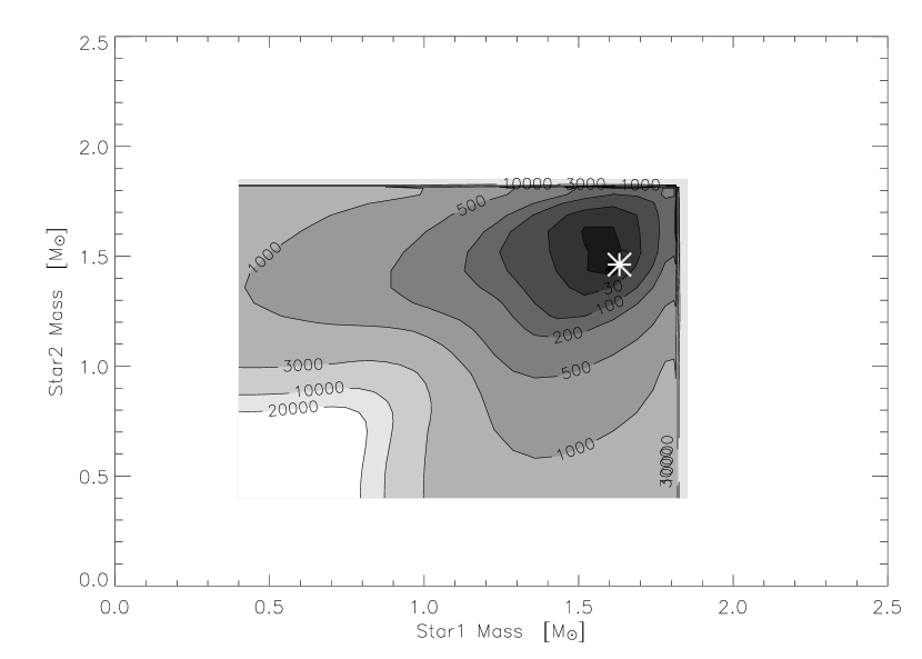
Figure 4: The MECI $\chi^{2}_{\nu}$ surface to the FS Monocerotis light curve and colors (Lacy et al. 2000), assuming an age of $1.6$ Gyr and fixing $w=10$. The estimate of the stellar masses (Lacy et al. 2000) from a combined analysis of the light curve and spectroscopic observations is indicated by a white asterisk, and is near to the minimum identified by MECI. Note the erratic behavior of the contours at the upper end of the mass range, which results from the rapid evolution of stars of those masses at this age.

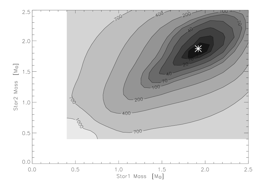
Figure 5: The MECI $\chi^{2}_{\nu}$ surface to the WW Camelopardalis light curve and colors (Lacy et al. 2002), assuming an age of $0.6$ Gyr and fixing $w=10$. The estimate of the stellar masses (Lacy et al. 2002) from a combined analysis of the light curve and spectroscopic observations is indicated by a white asterisk, and is extremely close to the solution identified by MECI.

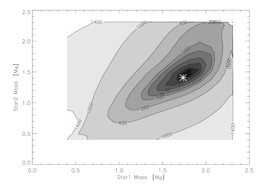
Figure 6: The MECI $\chi^{2}_{\nu}$ surface to the BP Vulpeculae light curve and colors (Lacy et al. 2003), assuming an age of $0.8$ Gyr and fixing $w=10$. The estimate of the stellar masses (Lacy et al. 2003) from a combined analysis of the light curve and spectroscopic observations is indicated by a white asterisk, and is extremely close to the solution identified by MECI.

We examined three well-studied EBs. The first was FS Monocerotis (Lacy et al., 2000), for which we modeled the published light curve, which had $N_{lc}=249$ data points, as well as the published $U-B$ and $B-V$ colors. The second was WW Camelopardalis (Lacy et al., 2002), for which we modeled the published light curve, which had $N_{lc}=5759$ observations, as well as the $B-V$ color. Finally, we studied BP Vulpeculae (Lacy et al., 2003), for which we modeled the published light curve, which had $N_{lc}=5236$ observations, as well as the $B-V$ color. All three published light curves were observed in $V$-band and are plotted in Figure 3. The colors had been corrected for reddening. The contour plots of the ${\chi}^{2}_{\nu}$ surfaces resulting from our MECI analysis (setting the weighting $w=10$) are shown in Figures 4, 5, and 6. Note that FS Mon is more tightly constrained due to its greater color information. Furthermore, the asymmetry in BP Vol’s contour is due to its unequal eclipse depths. In all cases, the ${\chi}^{2}_{\nu}$ surface has a single minimum, which is close to the published values. In Table 1, we tabulate the results of our analysis and compare these to the published values.

We then changed the weighting factor to $w=100$ and repeated this procedure. The MECI results for FS Mon and BP Vul were essentially identical to our earlier findings for $w=10$. In the case of WW Cam, the results for $w=10$ were significantly closer to the published values. This is likely due to the fact that it is a young system ($age=500$ Myr), for which the brightness and radii at constant mass vary significantly. Thus, the lower light curve information weighting brought about smoother $\chi^{2}_{\nu}$ contours (see §3.3).

4.2 Simulated systems

In our second test, we produced large numbers of simulated EB light curves with various levels of injected noise, and subsequently analyzed these photometric datasets with MECI. We then compared the input and derived estimates of the stellar masses and ages in order to quantify the accuracy of the MECI analysis.

We selected the orbital and stellar parameters of each simulated EB as follows. First, we drew an age at random from a uniform probability distribution between $200$ Myr and $10$ Gyr. We then selected the masses of the two EB components independently from a flat distribution from $0.4M_{\odot}$ and the maximum mass at which stars of this age would still be located on the main-sequence. We then assigned the orbital period by drawing a number from a uniform probability distribution spanning $0<P\leq 10$ days. Similarly, we assigned the epoch of perihelion by drawing from a uniform probability distribution spanning $0\leq t_{0}<P$, and the orbital inclination from a uniform distribution within the range that produces eclipses, $\arccos(r_{1}+r_{2})\leq i\leq{\pi}/2$. For the tests of eccentric systems, we also randomly selected an eccentricity, uniformly from $0\leq e\leq 0.1$, and randomly selected the angle of perihelion, uniformly from $0\leq\omega<2{\pi}$. Finally, we rejected any EB system if its components were overlapping or in near contact, $r_{1}+r_{2}\geq 0.8$. We also filtered out EBs with undersampled eclipses, or for which one of the eclipse depths was smaller than the assumed $1\,\sigma$ noise level.

Each simulated light curve contained 1000 $R$-band data points, to which we injected Gaussian-distributed noise. When color information was required, we computed the out-of-eclipse photometric colors for each EB, and injected a $0.02$ mag Gaussian-distributed error to this value. The colors we considered were $(V-I)_{Cousins}$, which is similar to the color provided by the OGLE II catalog (Wozniak et al., 2002), as well as $(J-H)_{ESO}$ and $(H-K)_{ESO}$, which are similar to the colors provided by the 2MASS catalog (Kleinmann et al., 1994).

We simulated 8 sets of 2500 systems each, with the sets differing in the following respects (see Table 2): (1) circular or eccentric orbits, (2) the number of points in the search grid, (3) the value of $w$, which describes the relative weight between the color and photometric data, and (4) the availability of color information.

In order to summarize the accuracy of the MECI results, we computed the quadrature sum of the relative differences between the assumed and derived values for the masses of the two components. We plot the histograms of these values in Figure 7. In each histogram, we identify the value encompassing the region that contains 90% of the results. We call this range the “$90^{th}$ percentile error”, and list it in the final column of Table 2.

We find that the inclusion of color information significantly improves the accuracy of the MECI results, lowering the $90^{th}$ percentile error from $30$% in set (A), to less than $6$% in sets (B) and (C). In contrast, changing the value of $w$ from $100$ in set (C), to $10$ in set (E), results in only a modest increase of $0.8$% in the size of the $90^{th}$ percentile error. This indicates that the results are robust to the particular choice of $w$. We note, however, that a value of $w>100$ will usually provide too little weight to the color information, which results in poorer accuracy. An extreme example of this is seen in set (A).

Similarly, MECI is not sensitive to the exact value of the search grid size. In particular, decreasing the grid size from $15\times 15$ in set (C), to $10\times 10$ in set (F), increases the $90^{th}$ percentile error only modestly, from $5.8$% to $6.1$%. This stability results from the fact that the $\chi^{2}_{\nu}$ function contains a broad minimum, which is well sampled even with $N=10$ grid points. We note, however, that this is no longer the case when considering evolved star systems (e.g. §3.3), for which a larger number of grid points is required.

When we decreased the level of the noise injected into the photometric time series from $0.01$ mag in set (C), to $0.001$ mag in set (D), the $90^{th}$ percentile error dropped from $5.8$% to $4.0$%. Surprisingly, the tail of the upper end of the error distribution extends to larger values in set (D). This appears to be due to the phenomenon discussed in §3.3, whereby the $\chi^{2}_{\nu}$ function occasionally contains many local minima. This problem becomes acute for eccentric systems, since they have a far more complex $\chi^{2}_{\nu}$ function. Decreasing their noise from $0.01$ mag in set (G), to $0.001$ mag in set (H), raises the $90^{th}$ percentile error from $8.8$% to $23$%. This relatively poor performance reflects the algorithm’s inability to robustly identify the global minimum under these conditions. In such cases one must increase the size of the search grid and iteratively solve for the orbital parameters of the systems, which results in a significant increase in the computational time.

4.3 Limitations

A significant degeneracy results for light curves in which two distinct eclipses are not apparent. For such systems, two distinct possibilities exist, namely that either the EB consists of two twin components with an orbital period $P$, or that the EB consists of two stars with very disparate sizes (such that the secondary eclipse is not discernable), with an orbital period $2\,P$. It is often necessary to flag such systems and conduct analyses with both possible values for the orbital periods. Distinguishing which of these possibilities is the correct solution is challenging, but in some instances there are clues. One such clue is a variable light curve plateau that results from the mutual tidal distortions, which in turn might indicate the true orbital period (twice that of the observed modulation). A second possibility is a red excess in the system color indicating a low-mass secondary. Of course, follow-up spectroscopic observations can readily resolve this degeneracy, either by indicating the presence of two components of similar brightness, or through a direct determination of the orbital period.

We note that MECI employs a simplified model for the generation of the light curves (DEBiL), which can bring about additional complications when applied to systems in which our assumptions (see §3.2) do not hold. For example, our model ignores the effect of third light, either from a physically associated star or a chance superposition, which reduces the apparent depths of the eclipses and may contaminate the estimate of the system color. Furthermore, we have ignored reflection effects, which can raise the light curve plateau at times immediately preceding or following eclipses. Finally, tidal distortions will increase the apparent system brightness at orbital quadrature, which can serve to increase the apparent depth of the eclipses. In order for MECI to be able to properly handle these cases, its light curve generator must be replace with a more sophisticated one (e.g. WD or EBOP), which will likely make MECI significantly more computationally expensive.

5 Conclusions

We have described a method for identifying an EB’s components using only its photometric light curve and combined colors. By utilizing theoretical isochrones and limb-darkening coefficients, this method greatly reduces the EB parameter space over which one needs to search. Using this approach, we can quickly estimate the masses, radii and absolute magnitudes of the components, without spectroscopic data. We described an implementation of this method, which enables the systematic analyses of datasets consisting of photometric time series of large numbers of stars, such as those produced by OGLE, MACHO, TrES, HAT, and many others. Such techniques are expected to grow in importance with the next generation surveys, such as Pan-STARRS (Kaiser et al., 2002) and LSST (Tyson, 2002). In a future publication, we shall describe a specific application of these codes, namely to search for low-mass eclipsing binaries in the TrES dataset.

Table 1: Accuracy of MECI parameter estimates for 3 well-studied binaries.

	MECI ($w=10$)			MECI ($w=100$)			Lacy et al. (2000, 2002, 2003)
System	Mass 1	Mass 2	Age	Mass 1	Mass 2	Age	Mass 1	Mass 2	Age
	$[M_{\odot}]$	$[M_{\odot}]$	$[Gyr]$	$[M_{\odot}]$	$[M_{\odot}]$	$[Gyr]$	$[M_{\odot}]$	$[M_{\odot}]$	$[Gyr]$
FS Monocerotis	1.58	1.47	1.6	1.57	1.47	1.6	1.632	1.462	1.6
($N_{lc}=249$)	[3.3%]	[0.5%]	[0.3%]	[3.6%]	[0.5%]	[0.1%]	$\pm 0.012$	$\pm 0.010$	$\pm 0.3$
WW Camelopardalis	1.92	1.86	0.5	2.10	2.02	0.4	1.920	1.873	0.5
($N_{lc}=5759$)	[0.2%]	[0.9%]	[3%]	[9.6%]	[8.0%]	[17%]	$\pm 0.013$	$\pm 0.018$	$\pm 0.1$
BP Vulpeculae	1.78	1.48	0.7	1.77	1.48	0.8	1.737	1.408	1.0
($N_{lc}=5236$)	[2.2%]	[5.3%]	[26%]	[1.9%]	[5.2%]	[22%]	$\pm 0.015$	$\pm 0.009$	$\pm 0.2$

Note. — The rightmost columns list the masses, ages, and errors of the component stars as determined by a combined analysis of their light curves and spectroscopic orbits (Lacy et al., 2000, 2002, 2003). The leftmost columns list the estimates of these quantities produced by MECI assuming $w=10$, and the central columns list the estimates from MECI assuming $w=100$. The square brackets indicate the fractional errors of the MECI results with respect to the numbers in the rightmost columns.

Table 2: Accuracy of MECI mass estimates for simulated systems.

Set	Noise	Orbit	Search grid	Weighting	Color information	$90^{th}$ percentile error
A	0.01 mag	circular	$15\times 15$	N/A	No color information	30%
B	0.01 mag	circular	$15\times 15$	$w=100$	$(V-I)_{Cousins}$	5.9%
C	0.01 mag	circular	$15\times 15$	$w=100$	$(J-H)_{ESO}$ and $(H-K)_{ESO}$	5.8%
D	0.001 mag	circular	$15\times 15$	$w=100$	$(J-H)_{ESO}$ and $(H-K)_{ESO}$	4.0%
E	0.01 mag	circular	$15\times 15$	$w=\ 10$	$(J-H)_{ESO}$ and $(H-K)_{ESO}$	6.6%
F	0.01 mag	circular	$10\times 10$	$w=100$	$(J-H)_{ESO}$ and $(H-K)_{ESO}$	6.1%
G	0.01 mag	eccentric	$15\times 15$	$w=100$	$(J-H)_{ESO}$ and $(H-K)_{ESO}$	8.8%
H	0.001 mag	eccentric	$15\times 15$	$w=100$	$(J-H)_{ESO}$ and $(H-K)_{ESO}$	23%

Note. — The parameters of the 8 distinct sets of simulated EB light curves that we generated and subsequently analyzed with MECI. The rightmost column lists the range of the quadrature sum of the fractional errors on the masses which encompasses 90% of the solutions (see Fig. 7), which we take to be indicative of the accuracy of MECI under the specified conditions.

Figure 2: A flow diagram demonstrating the process by which MECI assigns the parameters to an EB based on its observed light curve. The details of stages 1 & 2 are described in §3.1 and §3.2, respectively.

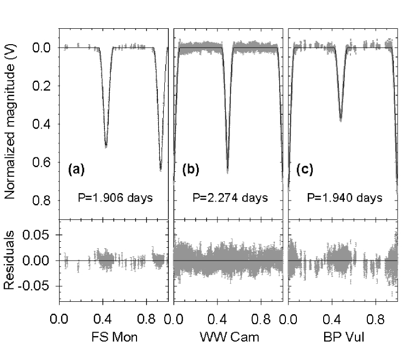
Figure 3: The observed light curves of FS Monocerotis (Lacy et al. 2000), WW Camelopardalis (Lacy et al. 2002), and BP Vulpeculae (Lacy et al. 2003), each overplotted with the best-fit model DEBiL solution used in our MECI algorithm. The masses and ages corresponding to these solutions are listed in Table 1. The residuals to each fit are shown in the lower panels. A high-quality version of this figure can be seen at:
http://cfa-www.harvard.edu/$\sim$jdevor/MECI/paper/

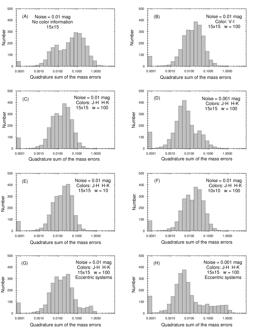
Figure 7: Each panel shows the histogram of the quadrature sum of the relative differences in the assumed and calculated masses for the stellar components, for each of the sets of simulated light curves described in Table 2. Each set contains $2500$ simulated EBs as described in §4.2, and the key parameters of each set are listed in the upper right corner of each panel. The leftmost bin contains the sum of all results with values less than 0.0001. The ability of the method to accurately assign the masses to the component stars degrades significantly in the absence of any color information (upper left panel), but is generally robust against changes in the particular choice of $w$ or $N$ (see §4.2).

References

- Alard et al. (1998) Alard, C. & Lupton, R. H. 1998, ApJ, 503, 325
- Alard (2000) Alard, C. 2000, A&AS, 144, 363
- Alcock et al. (1997) Alcock, C., et al. 1997, AJ, 114, 326
- Alcock et al. (1998) Alcock, C., et al. 1998, ApJ, 492, 190
- Alonso et al. (2004) Alonso, R., et al. 2004, ApJ, 613, L153
- Andersen (1998) Andersen, J. 1998, IAU Symp. 189: Fundamental Stellar Properties, 189, 99
- Bakos et al. (2004) Bakos, G., Noyes, R. W., Kovács, G., Stanek, K. Z., Sasselov, D. D., & Domsa, I. 2004, PASP, 116, 266
- Baraffe et al. (1998) Baraffe, I., Chabrier, G., Allard, F., & Hauschildt, P. H. 1998, A&A, 337, 403
- Carpenter (2001) Carpenter, J. M. 2001, AJ, 121, 2851
- Charbonneau et al. (2006) Charbonneau, D., Brown, T. M., Burrows, A., & Laughlin, G. 2006, in Protostars and Planets V, ed. B. Reipurth, D. Jewitt, & K. Keil, (Tucson: University of Arizona Press), in press, astro-ph/0603376
- Claret et al. (1995) Claret, A., Diaz-Cordoves, J., & Gimenez, A. 1995, A&AS, 114, 247
- Claret (1998) Claret, A. 1998, A&A, 335, 647
- Claret (2000) Claret, A. 2000, A&A, 363, 1081
- Creevey et al. (2005) Creevey, O. L., et al. 2005, ApJ, 625, L127
- Crotts (1992) Crotts, A. P. S. 1992, ApJ, 399, L43
- Delfosse et al. (1999) Delfosse, X., Forveille, T., Mayor, M., Burnet, M., & Perrier, C. 1999, A&A, 341, L63
- Devor (2004) Devor, J. 2004, American Astronomical Society Meeting Abstracts, 205
- Devor (2005) Devor, J. 2005, ApJ, 628, 411
- Devor & Charbonneau (2005) Devor, J., Charbonneau, D. 2005, astro-ph/0510067
- Duquennoy & Mayor (1991) Duquennoy, A., & Mayor, M. 1991, A&A, 248, 485
- Etzel (1981) Etzel, P. B. 1981, in Photometric and Spectroscopic Binary Systems (Dordrecht: Reidel)
- Etzel (1991) Etzel, P. B. 1991, International Amateur-Professional Photoelectric Photometry Communications, 45, 25
- Girardi et al. (2004) Girardi, L., Grebel, E. K., Odenkirchen, M., & Chiosi, C. 2004, A&A, 422, 205
- Guinan et al. (1996) Guinan, E. F., Bradstreet, D. H., & Dewarf, L. E. 1996, ASP Conf. Ser. 90: The Origins, Evolution, and Destinies of Binary Stars in Clusters, 90, 196
- Kaiser et al. (2002) Kaiser, N., et al. 2002, Proc. SPIE, 4836, 154
- Kallrath & Milone (1999) Kallrath, J., & Milone, E. F. 1999, Eclipsing binary stars : modeling and analysis / Joseph Kallrath, Eugene F. Milone. New York : Springer, 1999. (Astronomy and astrophysics library), 169
- Kim et al. (2002) Kim, Y., Demarque, P., Yi, S. K., & Alexander, D. R. 2002, ApJS, 143, 499
- Kleinmann et al. (1994) Kleinmann, S. G., et al. 1994, Ap&SS, 217, 11
- Kopal (1959) Kopal, Z. 1959, The International Astrophysics Series, London: Chapman & Hall, 1959
- Kron (1952) Kron, G. E. 1952, ApJ, 115, 301
- Kurucz (1992) Kurucz, R. L. 1992, IAU Symp. 149: The Stellar Populations of Galaxies, 149, 225
- Lacy (1977a) Lacy, C. H. 1977a, ApJS, 34, 479
- Lacy (1977b) Lacy, C. H. 1977b, ApJ, 218, 444
- Lacy et al. (2000) Lacy, C. H. S., Torres, G., Claret, A., Stefanik, R. P., Latham, D. W., & Sabby, J. A. 2000, AJ, 119, 1389
- Lacy et al. (2002) Lacy, C. H. S., Torres, G., Claret, A., & Sabby, J. A. 2002, AJ, 123, 1013
- Lacy et al. (2003) Lacy, C. H. S., Torres, G., Claret, A., & Sabby, J. A. 2003, AJ, 126, 1905
- Latham (1992) Latham, D. W. 1992, ASP Conf. Ser. 32: IAU Colloq. 135: Complementary Approaches to Double and Multiple Star Research, 32, 110
- Maceroni & Rucinski (1997) Maceroni, C., & Rucinski, S. M. 1997, PASP, 109, 782
- Maceroni & Montalbán (2004) Maceroni, C., & Montalbán, J. 2004, A&A, 426, 577
- Mazeh et al. (2005) Mazeh, T., Tamuz, O., North, P. 2005, Close Binaries in the 21st Century: New Opportunities and Challenges, 45
- Metcalfe et al. (1996) Metcalfe, T. S., Mathieu, R. D., Latham, D. W., & Torres, G. 1996, ApJ, 456, 356
- McCullough et al. (2006) McCullough, P. R., et al. 2006, ApJ, in press, astro-ph/0605414
- Nelder (1965) Nelder, J. A., & Mead 1965, R., Computer Journal, 7, 308
- O’Donovan et al. (2006) O’Donovan, F. T., et al. 2006, astro-ph/0603005
- Paczynski (1997) Paczynski, B. 1997, The Extragalactic Distance Scale, 273
- Popper & Etzel (1981) Popper, D. M. & Etzel, P. B. 1981, AJ, 86, 102
- Pourbaix et al. (2004) Pourbaix, D., et al. 2004, A&A, 424, 727
- Press et al. (1992) Press, W. H., Teukolsky, S. A., Vetterling, W. T., & Flannery, B. P. 1992, (2nd ed.; Cambridge: University Press)
- Ribas (2003) Ribas, I. 2003, A&A, 398, 239
- Schwarzenberg-Czerny (1989) Schwarzenberg-Czerny, A. 1989, MNRAS, 241, 153
- Schwarzenberg-Czerny (1996) Schwarzenberg-Czerny, A. 1996, ApJ, 460, L107
- Stebbing (1910) Stebbing, J. 1910, ApJ, 32, 185
- Torres & Ribas (2002) Torres, G., & Ribas, I. 2002, ApJ, 567, 1140
- Tyson (2002) Tyson, J. A. 2002, Proc. SPIE, 4836, 10
- Udalski et al. (1994) Udalski, A., et al. 1994, Acta Astronomica, 44, 165
- Vallée (2005) Vallée, J. P. 2005, AJ, 130, 569
- Wilson & Devinney (1971) Wilson, R. E. & Devinney, E. J. 1971, ApJ, 166, 605
- Wambsganss (2006) Wambsganss, J. 2006, in Proc. of the 33rd Saas-Fee Advanced Course “Gravitational Lensing: Strong, Weak and Micro”, ed. G. Meylan, P. Jetzer, & P. North (Heidelberg: Springer-Verlag), 457
- Wozniak (2000) Wozniak, P. R. 2000, Acta Astronomica, 50, 421
- Wozniak et al. (2002) Wozniak, P. R., Udalski, A., Szymanski, M., Kubiak, M., Pietrzynski, G., Soszynski, I., & Zebrun, K. 2002, Acta Astronomica, 52, 129
- Wyithe & Wilson (2001) Wyithe, J. S. B. & Wilson, R. E. 2001, ApJ, 559, 260
- Wyithe & Wilson (2002) Wyithe, J. S. B. & Wilson, R. E. 2002, ApJ, 571, 293