The Dark Side and its Nature

Abstract

Although the cosmic concordance cosmology is quite successfull in fitting data, fine tuning and coincidence problems apparently weaken it. We review several possibilities to ease its problems, by considering various kinds of dynamical Dark Energy and possibly its coupling to Dark Matter, trying to set observational limits on Dark Energy state equation and coupling.

1.  Introduction

Until a decade ago two options were in competition: the world could be either SCDM or 0CDM. The former cosmology had matter density and deceleration parameters $\Omega_{om}\simeq 1$ and $q_{o}=0.5$; the latter had $\Omega_{om}\simeq 0.2$–0.3 and $q_{o}\sim 0\,$. $\Omega_{om}\simeq 1$ was supported by COBE data and agreed with generic inflationary predictions; $\Omega_{om}\simeq 0.3$ was supported by evolutionary data and inflation made it acceptable without horrible fine tunings. When data became too far from SCDM, the mixed model variant valda became popular.

Then SNIa data riepea required $q_{o}\sim-0.6$–0.7. $\Omega_{om}$ could still be $\simeq 0.3$ if the gap up to $\Omega_{o}=1$ was covered by a substance with $p\simeq-\rho$, the Dark Energy (DE). The $\Lambda$CDM models, considered until then little more than a smart counter–example, begun their fast uprise to become the Cosmic Concordance Cosmology (CCC). Then, soon after SNIa data, deep sample analysis deep and fresh CMB data cmb converged in confirming that $\Omega_{om}\simeq 0.3$ with $\Omega_{o}\simeq 1\,$ and the CCC became a must.

Only a minority were however happy with $\Lambda$ being the cosmological constant. Thus, CCC brought the problem of DE nature. Most of this paper deals with DE being a self–interacting field, either fully decoupled or decoupled from any other component apart Dark Matter (DM): dynamical and coupled DE (dDE and cDE), respectively.

Fig. 1 illustrates why we favor these options. If DE pressure and density meet the condition $p_{de}=-\rho_{de}\,$ exactly, then $\rho_{de}$ is constant: backward in time, DE rapidly becomes negligible and we wonder why just today it became relevant. This is the coincidence problem. But, if DE is false vacuum, at the end of the transition, $\rho_{de}$ should have became $\sim 1:10^{54}$ of its pre–transition value. This is a typical fine tuning problem.

The latter problem vanishes in dDE models. In the interaction potential no fine–tuned scale appears. However, as shown in panel dDE, the coincidence problem is not eased. Then, if DE suitably interacts with DM, densities can evolve as in panel cDE, and also the coincidence problem is eased: DE and DM have had comparable densities since long.

We became accustomed to cosmologies with various components of similar density, e.g., baryons and DM. CCC now requires also DE to fall in the same range. This would not be an extra requirement if DE and DM are just two different aspects of a Dark Side, their interaction being a signature of a common nature. An example is the dual axion model dual , but here we approach the question from the phaenomenological side.

We outline soon that DM–DE coupling predicts a significant baryon–DM segregation in non–linear structures. Hydrodynamics succeeds in explaining most segregation effects observed in the real word, by tuning suitable parameters. If the required tunings conflict with other data or other observations require a different behavior of baryons and DM still before the onset of hydro, the DM–DE coupling would find an observational support.

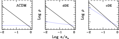
Figure 1: DM and DE densities in $\Lambda$CDM, dDE amd cDE cosmologies. The solid (dotted) line shows DM (DE) densities in the different classes of models.

Constraints on cDE from CMB data were first discussed by amendola . In Section 2 the results of a fit to WMAP1 data colombo1 are reported. Discussing non–linear constraints is a harder task. Even predictions based on the Press & Schechter or Sheth & Tormen PSST formalism are hard to obtain. In Section 3 we shall explain why it is so. In Section 4 we shall then use ST expressions to predict mass functions. Our conclusions are in Section 5.

2.  Background and linear fluctuations . If DE is a scalar field $\phi$, self–interacting through a potential $V(\phi)$ wetterich , RP , it is

$$\rho_{de}=\rho_{k,de}+\rho_{p,de}\equiv{{\dot{\phi}}^{2}/2a^{2}}+V(\phi),~{}~{}~{}~{}~{}~{}~{}p_{de}=\rho_{k,de}-\rho_{p,de}\equiv w\,\rho_{de}~{}.$$ (1)

Then, if dynamical equations yield $\rho_{k,de}/V\ll 1/2$, it is $-1/3\gg w>-1$. We use the background metric $ds^{2}=a^{2}(\tau)(-d\tau^{2}+dx_{i}dx^{i})$; dots indicate differentiation with respect to $\tau$ (conformal time). This DE is dubbed dynamical (dDE) and much work has been done on it, also aiming at restricting the range of acceptable $w(\tau)$’s, so gaining an observational insight onto the physics responsible for the potential $V(\phi)$.

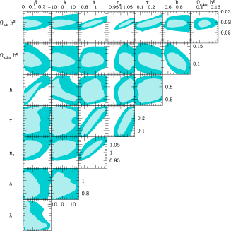
Figure 2: 1– and 2–$\sigma$ limits on model parameters, obtained from a MCMC fit of dDE and cDE (SUGRA) cosmologies with WMAP1. Here $\lambda=\log_{10}(\Lambda/{\rm GeV})$; $A$, $n_{s}$, $\tau$ are fluctuation amplitude, primeval spectral index, opacity. $\Lambda$ turns out to be substantially unconstrained. For dDE, $n_{s}$ is greater than for $\Lambda$CDM, but all parameter values are compatible with $\Lambda$CDM values within $\sim 2$ $\sigma$’s. For cDE, the coupling $\beta$, at 2–$\sigma$, should be $<\sim 0.3$.

In this paper we shall consider the potentials

$SUGRA:~{}~{}V(\phi)=(\Lambda^{\alpha+4}/\phi^{\alpha})\exp(4\pi\phi^{2}/m_{p}^{2})~{},~{}~{}~{}~{}~{}RP:~{}~{}V(\phi)=\Lambda^{\alpha+4}/\phi^{\alpha}~{}$

(brax , RP ), admitting tracker solutions and yielding two opposite $w(\tau)$ behaviors: nearly constant for RP, fastly varying for SUGRA. Then, the effects we find should not be related to the shape of $V(\phi)$ but to the coupling. Most results are shown for $\Lambda=10^{2}\,$GeV; minor shifts occur when varying $\log_{10}(\Lambda/{\rm GeV})$ in the 1–4 range.

DM–DE coupling, fixed by a suitable parameter $\beta$, modifies background equations for DE and DM as well as those ruling density perturbations (see, e.g., amendola ).

Linear codes, modified by in this way allow predictions on CMB anisotropies and polarization. In this way we fitted dDE and cDE models to WMAP1 data colombo1 . In Figs. 2 MCMC limits on model parameters are shown, for the dDE and cDE with SUGRA potential. The $\chi^{2}$ (likelihhod) is 1.066 (4.7$\,\%$) both for $\Lambda$CDM and cDE, 1.064 (5$\,\%$) for dDE, with a marginal improvement. More significantly, cDE is not worse than $\Lambda$CDM.

3.  Non–linear Newtonian approximation

While CMB analysis is based on linearized eqs., if we deal with scales well below the horizon and non–relativistic particles, the restriction $\delta_{c,b}\ll 1$ can be lifted. An alternative Newtonian approximation is then licit, within which tensor gravity and scalar field cause overlapping effects adequately described by assuming:

(i) DM particle masses to vary, so that $M_{c}(\tau)=M_{c}(\tau_{i})\exp[-C(\phi-\phi_{i})].$

(ii) Gravity between DM particles to be set by $G^{*}=\gamma G$.

Here $C=\sqrt{16\pi G/3}~{}\beta~{},~{}~{}\gamma=1+4\beta^{2}/3$ (see, e.g., maccio ). This approach allowed us to study spherical top–hat fluctuations mainini6 , so predicting the cluster mass functions in cDE models maibon6 , and to perform n–body simulations maccio .

The main novel feature of cDE cosmologies we outline in this way is DM–baryon segregation, a strong effect, visible in the evolution of a spherical top–hat fluctuation.

Although in all cosmologies, apart SCDM, the spherical growth must be studied numerically, in cDE, just because of the ongoing segregation, the numerical approach is essential. In all cases apart cDE, the only variable describing a top–hat is its radius $R$, set to expand initially as scale factor $a$. Then, the greater density inside the top hat slows down $R$ in respect to $a$, so that the decreasing $\rho(<R)$ increases in respect to the average $\rho$. At a time $t_{ta}$, when $\Delta=\rho(<R)/\rho$ attains a suitable value $\chi$, $R$ starts decreasing, to formally vanish within a finite time $t_{c}$. For sCDM, $\chi=(3\pi/4)^{2}$ and $t_{c}/t_{ta}=2$. In other non–cDE models, $\chi$ and $t_{c}/t_{ta}$ take slightly different values.

However, when $\rho(<R)$ increases, unless the heat produced by the $p\,dV$ work is radiated, virial equilibrium is soon attained, and any realistic fluctuation stops contracting at a radius $R_{v}$. In sCDM, $R_{v}/R_{ta}=1/2$ and, taking into account the symultaneous growth of $a$, the virial density contrast is then $\Delta_{v}=32\chi\simeq 180$, indipendently of $t_{c}$. Values are slightly different for other $\Lambda$CDM and dDE and a usual assumption is that the system relaxes into its virialized configuration just within $t_{c}$.

$\Delta_{v}$ values for $\Lambda$CDM and dDE were obtained by Lahav_brian and io ; collapse1 , respectively. The same problem was treated in mainini6 for cDE. In this case, $R_{b}$ and $R_{c}$ (baryon and DM radii) initially grow as the scale factor, but $R_{b}$ soon exceeds $R_{c}$, because of the stronger effective gravity; peripheral baryons then leak out from $R_{c}$, so that DM no longer feels their gravity, while baryons above $R_{c}$ feel the gravity also of external DM layers. Then, above $R_{c}$, the baryon profile is no longer top–hat, while a fresh perturbation in DM arises. Re–contraction will then start at different times for different components and layers. Similarly, virialization conditions are fulfilled earlier by inner layers, although outer layer fall–out shall later perturb them so that the onset of virial equilibrium is a multi–stage process. Furthermore, when the external baryons fall–out onto the virialized core, richer of DM, they are accompanied by DM materials originally outside the top–hat, perturbed by baryon over–expansion.

Each layer and substance, in such system, feels a different force; each shell needs then to be considered separately; this is why the numerical problem is far more intricate.

Figure 3: Density profiles at different $a$ values for $\beta=0.2$ model. Notice the progressive deformation of the baryon profile (dotted lines) in respect of the DM profile (solid line).

The collapse stops at virialization. Fig. 3 assumes the growth to stop when all DM originally in the top–hat, and baryons inside it, virialize. Already at $a=0.2$, before the turn–around, the baryon top–hat boundary is no longer vertical. At $a=0.6$ ($\sim$turn–around), a similar effect is visible also for DM. The effect is even more pronounced at $a_{vir}\simeq 0.92$. The same effects, just slightly weeker, are present also for $\beta=0.05$

Fig. 3 shows also that baryons leak out from the DM top–hat. For $a\sim 0.92$, when DM and inner baryons virialize, $\sim 10\,\%$ ( $\sim 40\,\%$) of baryons are out of the top–hat, if $\beta=0.05$ ($\beta=0.2\,$). These values increase by an additional $10\,\%$ in the RP case.

The virialization of materials within $R$ requires that $2\,T(<R)=R\,dU(<R)/dR\,$. Kinetic and potential energies have fairly straightforward expressions. The only point to outline is that DM–DE energy exchanges, for the background, are accounted for by background evolution eqs., so that, when fluctuations are considered, the background contribution must not considered again.

4.  Mass functions in cDE theories

Let us compare the actual growth of a top–hat fluctuation with its growth if we assume linear equations to hold, indipendently of its amplitude. While the real fluctuation abandons the linear regime, turns–around, recontracts and recollapses at the time $\tau_{rc}$, linear equations let that fluctuation steadily grow, up to an amplitude $\delta_{rc}$ at the time $\tau_{rc}$.

The linear evolution does not affect amplitude distributions. If they are initially distributed in a Gaussian way, at $\tau_{rc}$ we can still integrate the Gaussian from $\delta_{rc}$, so finding the probability that an object forms and virializes. This is the basic pattern of the PS–ST approach, that we apply also to cDE cosmologies. For them, however, $\tau_{rc}\,$ is different for DM and baryons. Viceversa, if we require $\tau_{o}$ to coincide with $\tau_{rc}$, we have two different linear amplitudes, $\delta_{rc}^{(b)}$ and $\delta_{rc}^{(c)}$, yielding recollapse at $\tau_{o}$ for all baryons or all DM.

The $\beta$ dependence of $\delta_{rc}^{(c,b)}$ at $z=0$ and their $z$ dependence are given in maibon6 . Setting $\nu_{M}=\delta_{M}/\sigma_{M}$, the PS differential mass function then reads

$$\psi(M)=\sqrt{2/\pi}(\rho/M)\int_{\delta_{rc}/\sigma_{M}}^{\infty}d\nu_{M}~{}(d\nu_{M}/dM)\,\nu_{M}\exp\{-\nu_{M}^{2}/2\}~{},$$ (2)

using here $\delta_{rc}^{(c)}$, $\delta_{rc}^{(b)}$, or any intermediate value, according to the observable to be fitted. The ST expression is obtainable from eq. (2) through the replacement

$\nu_{M}\exp(-{\nu_{M}^{2}\over 2})\to{\cal N}^{\prime}\,{\nu^{\prime}}_{M}(1+{\nu^{\prime}}_{M}^{-3/5})\,\exp(-{{\nu^{\prime}}_{M}^{2}\over 2})$,  with ${\cal N}^{\prime}=0.322,~{}{\nu^{\prime}}^{2}_{M}=0.707\,\nu^{2}_{M},$

meant to take into account the effects of non–sphericity in the halo growth.

In $\Lambda$CDM or dDE, the mass $M$ in ST expressions is the mass originally in the top–hat. In cDE, indipendently of the value taken for $\delta_{cr}$, virialized systems will be baryon depleted. In fact, mass function built by taking $\delta_{cr}^{c}$, concern objects before a part of the initial baryon content has fallen out. But, even if we wait for a total or partial baryon fall out, by using $\delta_{cr}^{b}$ or an intermediate value, the initial baryons come back carrying with them DM layers initially external to the top–hat. A prediction of cDE theories, therefore, is that $\Omega_{c}/\Omega_{b}$, measured in any virialized structure, exceeds the background ratio.

Figure 4: Cluster mass function at $z=0$. Four models are considered: $\Lambda$CDM, SUGRA dDE with $\Lambda=100\,$MeV, and two SUGRA cDE with $\beta=0.2$ and 0.05. Dashed areas are limited by the mass functions for $\delta_{c,rc}^{(c)}$ or $\delta_{c,rc}^{(b)}$ in cDE models. The lower panel yields ratios in respect to $\Lambda$CDM. The r.h.s. panel overlaps cDE results for SUGRA and RP.

We shall plot mass functions obtained using either $\delta_{c,rc}^{(c)}$ or $\delta_{c,rc}^{(b)}$. Actual data should fall in the interval between these functions. If, during the process of cluster formation, outer layers were stripped by close encounters, data shall be closer to the $\delta_{c,rc}^{(c)}$ curve.

Figure 4 shows $n(>$$M)=\int_{M}^{\infty}dM^{\prime}\,\psi(M^{\prime})$ obtained through eq. (2). The lower panel shows the ratio between halo numbers for each model and $\Lambda$CDM. No large differences between $\Lambda$CDM and dDE are found at $z=0\,$. Shifts are greater between $\Lambda$CDM and cDE. For $\beta=0.20$, clusters with $M>\sim 3\cdot 10^{14}h^{-1}M_{\odot}$ are half than in $\Lambda$CDM. For $\beta=0.05$ the shift is smaller, hardly reaching $20\,\%$, still opposite to dDE. The r.h.s. panel shows that these features are true also for RP. More RP results can be found in maibon6 .

Figure 5: Number of clusters with $M>10^{14}h^{-1}M_{\odot}\,$ (left panel) or $4\cdot 10^{14}h^{-1}M_{\odot}\,$ (right panel) in a fixed solid angle and redshift interval. The upper linear (lower log) plot outlines shifts at small (large) $z$.

To discriminate between models, cluster evolution predictions should provide numbers per solid angle and redshift interval (rather than for comoving volumes, see sole ) as in the upper panels of Fig. 5. In the lower panels, SUGRA models and $\Lambda$CDM are compared. We consider two masses: $10^{14}$ and $4\cdot 10^{14}h^{-1}M_{\odot}$; for the latter scale, a magnified box shows the expected low–$z$ behavior showing how we pass from numbers smaller than $\Lambda$CDM to greater numbers, for $\beta=0.05$, at a redshift $z\simeq 0.7\,$. The high–$z$ behaviors for $\beta=0.05$ or 0.2 lay on the opposite sides of $\Lambda$CDM.

5.  Conclusions

In this paper we discussed individual cluster formation and cluster mass functions. A first finding is the expected baryon–DM segregation causing baryon depletion in clusters. Depletion could be even stronger if the outer layers are stripped out by close encounters during the formation process. Preliminary results of simulations confirm these outputs.

As far as mass functions are concerned, a first significant feature is that the discrepancy of dDE from $\Lambda$CDM is partially or totally erased by a fairly small DM–DE coupling, and many cDE predictions lay on the opposite side of $\Lambda$CDM, in respect to dDE.

At $z=0$, a shortage of large clusters is expected in cDE. Therefore, if $\Lambda$CDM is used to fit data in a cDE world, cluster data yield a $\sigma_{8}$ smaller than galaxy data.

When we consider the $z$ dependence, we see that (i) when passing from $\Lambda$CDM to uncoupled SUGRA, the cluster number is expected to be greater. (ii) When coupling is added, the cluster number excess is reduced and the $\Lambda$CDM behavior is reapproached. (iii) A coupling $\beta=0.05$ may still yield result on the upper side of $\Lambda$CDM, while $\beta=0.2$ displaces the expected behavior well below $\Lambda$CDM.

This can be fairly easily understood. When $\rho_{de}$ keeps constant, while $\rho_{m}\propto(1+z)^{3}$, DE relevance rapidly fades. In dDE models, instead, $\rho_{de}$ (slightly) increases with $z$ and, to get the same amount of clusters at $z=0$, they must be there since earlier. Coupling acts in the opposite way, as gravity is boosted by the $\phi$ field. In the newtonian language, this means greater gravity constant ($G^{*}$) and DM particle masses at high $z$, speeding up cluster formation: a greater $\beta$ needs less clusters at high $z$ to meet their present number.

The overall result we wish to outline, however, is that non linearity apparently boosts the impact of coupling so that there are quite a few effects from which the coupling between DM and DE can be gauged. Most of them are just below the present observational threshold and even slight improvements of data precision will begin to allow discriminatory measurements. An essential step to fully exploit such data will be performing n–body and hydro simulations of cDE models. Through this pattern we can therefore expect soon more information on the actual nature of the Dark Side.

References

- (1) Bonometto S.A. & Valdarnini R., 1984, Ph.Lett.A 103, 369
- (2) Riess A.G. et al., 1998, AJ 116, 1009; Perlmutter S. et al, 1999, ApJ 517, 565; Astier P. et al., 2006, A&A 447, 31
- (3) Colless M.M. et al., MNRAS 329, 1039 Lovedai J. and SDSS collaboration, 2002, Contemp.Phys. 43, 437; Tegmark M. et al., 2004, ApJ 606, 702; Adelman–McCarty J.K. et al., 2006, ApJ S. 162, 38
- (4) de Bernardis P. et al., 2000, Nature 414, 955; Padin S. et al., 2001, ApJ 549, L1; Kovac J. et al., 2002, Nature 420, 772; Scott P.F. et al., 2003, MNRAS 341, 1076; Jarosik N. et al., 2006, astro-ph/0603452
- (5) Mainini R., Bonometto S.A., 2004, PRL 93, 121301; Mainini R., Colombo L. & Bonometto S.A., 2005, ApJ 635, 691-705
- (6) Amendola L., 1999, PR D 60, 043501; Amendola L. & Quercellini C., 2003, PR D 69; Amendola L., 2004,PR D 69, 2004, 103524
- (7) Colombo L. & Gervasi M., JCAP (in press) and astro-ph/0607262
- (8) Press W.H. & Schechter P., 1974, ApJ 187, 425; Sheth R.K. & Tormen G., 1999 MNRAS 308, 119; Sheth R.K. & Tormen G., 2002 MNRAS 329, 61; Jenkins, A., Frenk C.S., White S.D.M., Colberg J.M., Cole S., Evrard A.E., Couchman H.M.P. & Yoshida N., 2001, MNRAS 321, 372
- (9) Wetterich C. 1988, Nucl.Phys.B 302, 668
- (10) Ratra B. & Peebles P.J.E., 1988, PR D 37, 3406; Peebles P.J.E & Ratra B., 2003, Rev.Mod.Ph.75, 559
- (11) Brax, P. & Martin, J., 1999, Phys.Lett. B468, 40; Brax P., Martin J., Riazuelo A., 2000, PR D 62, 103505; Brax, P. & Martin, J., 2001, PR D 61, 10350.
- (12) Maccio’ A. V., Quercellini C., Mainini R., Amendola L., Bonometto S. A., 2004 PR D 69, 123516
- (13) Mainini R., 2005, PR D 72, 083514
- (14) Mainini R. & Bonometto S.A. 2006, PR D 74, 043504
- (15) Lahav, O., Lilje, P.R., Primack, J.R. & Rees, M., 1991, MNRAS 282, 263; Brian, G. & Norman, M., 1998, ApJ 495, 80
- (16) Mainini R., Macciò A., & Bonometto S.A., 2003, N.Astr. 8, 172; Mainini R., Macciò A., Bonometto S.A. & Klypin A. 2003, ApJ 599, 24
- (17) Wang L. & Steinhardt P.J., 1998, ApJ 508, 483; Horellou C., Berge J., 2005, astro-ph/0504465; Nunes N. J., da Silva A. C., Aghanim N., 2005, astro-ph/0506043
- (18) Solevi P., Mainini R., Bonometto S., Maccio’ A., Klypin A., Gottloeber S., 2006, MNRAS 366, 1346