A multi–wavelength study of the IRAS Deep Survey galaxy sample

Abstract

Context. The luminosity function (LF) is a basic tool in the study of galaxy evolution since it constrains galaxy formation models. The earliest LF estimates in the IR and far-IR spectral ranges seem to suggest strong evolution. Deeper samples are needed to confirm these predictions. We have a useful IR dataset, which provides a direct link between IRAS and ISO surveys, and the forthcoming deeper Spitzer Space Telescope and Akari cosmological surveys, to address this issue.

Aims. This allows us to derive the 60 $\mu$m local LF to sensitivity levels 10 times deeper than before, to investigate evolutionary effects up to a redshift of 0.37, and, using the 60/15$\mu$m bi-variate method, the poorly known 15 $\mu$m local LF of galaxies.

Methods. We exploited our ISOCAM observations of the IRAS Deep Survey (IDS) fields (Hacking & Houck 1987), to correct the $60\,\mu$m fluxes for confusion effects and observational biases. We find indications of a significant incompleteness of the IDS sample, still one of the deepest far-IR selected galaxy samples, below $\simeq 80\,$mJy (Mazzei et al. 2001). We have reliable identifications and spectroscopic redshifts for 100% of a complete subsample comprising 56 sources with $S(60\mu\hbox{m})>80\,$mJy.

Results. With our spectroscopic coverage we construct the 60 $\mu$m LF for a sample complete down to 80 mJy. This LF extends over three orders of magnitude in luminosity, from 9 up to more than 12 in $\log(L_{60}/L_{\odot})$. Despite the fact that the redshift range of our sample exceeds $z=0.3$, the $V/V_{max}$ test gives $<V/V_{max}>=0.51\pm 0.06$, consistent with a uniform distribution of sources. A more direct test, whereby the LF was measured in each of four different redshift intervals, does not point out any signature of evolution. On the other hand, the rest–frame 15$\mu$m local LF we derive, extends up to $\log(L_{15}/L_{\odot})=12$ and predicts 10 times more sources at $\log(L_{15}/L_{\odot})=11$ than are seen by Pozzi et al. (2004).

1 Introduction

Understanding how galaxies form and evolve is a key goal of modern physical cosmology. A fundamental observable of galaxies is their luminosity function (LF) which has long been used to constrain galaxy formation models and to quantify star formation and evolution both in luminosity and in density. The IR and far-IR spectral ranges are the best to deepen our knowledge of this subject since they trace the star formation that is responsible for galaxy formation. In particular several satellite missions, in the past (IRAS and ISO), and in the present (Spitzer, Akari), provided and will provide data which will be complementary for a detailed study of the LFs in such spectral domains.

The earliest IR estimate of the LFs, derived from the IRAS data (Rowan-Robinson et al., 1987; Saunders et al., 2000), indicated strong evolution, so that LF increases with redshift $\propto(1+z)^{3\pm 1}$. Moreover deep surveys at 15$\mu$m carried out with ISO (i.e., Elbaz et al., 1999; Flores, 1999; Lari et al., 2001; Metcalfe et al., 2003) seem to require, indeed, strong evolution of 15$\mu$m sources (Lagache et al. (2005) and references therein). Several evolutionary models were developed to explain these results, (e.g., Franceschini et al., 2001; Rowan-Robinson, 2001) and fit the IR/submillimiter source counts with different degrees of success. Nevertheless none of them is based on a local LF obtained from 15$\mu$m data, since the only available data until recently came from IRAS 12$\mu$m photometry (Rush et al., 1993; Xu, 1998; Fang et al., 1998). The first attempt to build up the 15$\mu$m LF of a NEPR subsample was made by Xu (2000). However he said that it must be considered as a preliminary work because: i) the sample of galaxies used is a incomplete sample, ii) there is a possible misidentification between the sources in the 60$\mu$m redshift survey of Ashby et al. (1996) and the 15$\mu$m sources in his work (see della Valle et al. (2006), for more details), iii) the model used to interpret the data treated all IR galaxies as a single population.

Our IDS/ISOCAM sample overcomes all these issues. It comprises a complete, 60$\mu$m selected sample of 56 galaxies in the North Ecliptic Polar Region (NEPR), a subsample of the original 98 IRAS Deep Survey (IDS) fields Hacking & Houck (1987).

The IRAS Deep Survey (IDS) sample was defined by co-adding IRAS scans of the North Ecliptic Polar Region (NEPR), representing more than 20 hours of integration time Hacking & Houck (1987). It comprises 98 sources with $S(60\mu\hbox{m})>50\,$mJy over an area of 6.25 square degrees.

Mazzei et al. (2001) exploited ISOCAM observations (range 12-18$\mu$m) of 94 IRAS Deep Survey (IDS) fields (Aussel et al., 2000), centered on the nominal positions of IDS sources, to correct the $60\,\mu$m fluxes for confusion effects and observational biases, finding indications of a significant incompleteness of the IDS sample below $\simeq 80\,$mJy. In della Valle et al (2006) we presented spectroscopic and optical observations of candidate identifications of our ISOCAM sources. Combining such observations with those by Ashby et al. (1996), we have reliable identifications and spectroscopic redshifts for 100% of the complete subsample comprising 56 sources with $S(60\mu\hbox{m})>80\,$mJy. It is the deepest complete IRAS selected sample available and still one of the deepest complete far-IR selected samples. For comparison, the IRAS Point Source Catalog (hereafter PSC; Beichman et al., 1988), comprises about $250,000$ IR sources with a completeness limit of 0.5 Jy at 60$\mu$m (Soifer et al., 1987). The deep ISOPHOT surveys, FIRBACK at 170$\mu$m, (Puget et al. 1999; Dole et al. 2001), and ELAIS at 90$\mu$m (Oliver et al., 2000) are all complete down to about 100 mJy. Moreover, the $70\,\mu$m Spitzer catalog of the 8.75 sq. deg. Bootes field is flux limited to 80 mJy (Dole et al. 2004) and the Spitzer extragalactic “main” First Look Survey, covering about 4 sq. deg., is complete to about 20 mJy at $70\,\mu$m (cf. Fig. 2 of Frayer et al. 2006), but redshift measurements are available for a substantial fraction of sources (yet only 72%) merely for $S_{70\mu{\rm m}}>50\,$mJy.

Thanks to our ISOCAM and optical/near-IR observations our sample, which provides a direct link between IRAS and ISO surveys, and the forthcoming deeper Spitzer Space Telescope and Akari cosmological surveys , is one of the far-IR selected complete samples with the larger spectral coverage. In addition to the ISOCAM and to the 60$\mu$m fluxes, most of them $\simeq$70% have 100$\mu$m fluxes, the remaining 30% with upper limits, and several ($\simeq$40%) have 25$\mu$m fluxes from IRAS Mazzei et al. (2001). Optical imaging has been already performed for 62.5% out of such a sample in at least one band, B or R, and for 34% in both the bands, moreover Two Micron All Sky Survey (2MASS) data are available for 68% of the sample and VLA observations for a large fraction of these sources are also available (Hacking et al., 1989).

In this paper, which is the second step of our multi-wavelength approach devoted to study the evolution of a far-IR selected sample of galaxies on which numerous studies of the far-IR evolution of galaxies still rely, we derive the 60$\mu$m luminosity function (LF) of such a sample. Our sample, ten times deeper in flux density than the PSC catalog, thus less liable to the effect of local density inhomogeneity, allows us to investigate evolutionary effects up to a redshift of 0.37, five times deeper than the PSCz catalog (z$\leq$ 0.07, Saunders et al., 2000). Moreover, we use the bi-variate method to translate the 60$\mu$m LF to the poorly known 15$\mu$m LF. We will compare our results with the recent determination of the 15$\mu$m local LF obtained by Pozzi et al. (2004) using the available data on the southern fields, S1 and S2, of the ELAIS survey Oliver et al. (2000).

The plan of the paper is the following: Section 2 focuses on far-IR properties of our complete sample, Section 3 shows our derived 60 $\mu$m LF, Section 4 presents the 15 $\mu$m LF based on the bi-variate 60/15 $\mu$m method. In Section 5 there are our conclusions.
Here and in the following we adopt: $\Lambda$=0.7, $\Omega_{b}$=0.3, $H_{0}$=70 km/s/Mpc.

2 The far-IR properties

Our complete sample comprises 56 IDS/ISOCAM sources. 25% out of these are beyond $z=0.1$, 12.5% beyond $z=0.15$ and only 5.3% at $z>0.2$ (Paper I). Such a sample is deeper than previous estimates Ashby et al. (1996), showing a tail extending up to z=0.375, almost 4 Gyr in look–back time.

Our morphological analysis (Bettoni et al., 2006) shows that, although 16% of our sources are multiple systems, unperturbed disk galaxies dominate the IDS/ISOCAM sample. One ULIRG, 3-53A, and two broad H$\alpha$ emission line galaxies with AGN optical properties (i.e., 3-70A and 3-96A, see Bettoni et al. (2006) for more details), are also included in the complete subsample.

Fig. 1 (left panel) shows the distribution of the far-IR luminosity ($L_{FIR}$, from 42.5 to 122.5  $\mu$m) of our sample, where $L_{FIR}=4\pi D_{L}^{2}$(FIR), FIR=1.26$\times 10^{-14}(2.58f_{60}+f_{100})$ W/m², and $f_{60}$ and $f_{100}$ are in Jy Helou et al. (1988). In such a figure, as in the following ones, K-corrections were derived from evolutionary population synthesis models taking into account dust effects Mazzei et al. (1995), luminosities were in units of solar bolometric luminosity, L${}_{\odot}=3.83\times 10^{33}$ erg/s. Moreover, upper limits to flux densities were accounted for by exploiting the Kaplan-Meier estimator Kaplan & Meier (1958). Calculations were carried out using the ASURV v 1.2 package Isobe & Feigelson (1990) which implements methods presented in Feigelson & Nelson (1985) and in Isobe et al. (1986). The Kaplan-Meier estimator is a non-parametric, maximum-likelihood-type estimator of the “true” distribution function (i.e., with all quantities properly measured, and no upper limits). The “survivor” function, giving the estimated proportion of objects with upper limits falling in each bin, does not produce, in general, integer numbers, but is normalized to the total number. This is why non-integer numbers of objects appear in the histograms of our figures.

The far-IR luminosity of the IDS/ISOCAM sample extends over 3 orders of magnitude (Fig. 1, left panel) with a mean value, $\log(L_{FIR})=10.2$, slightly lower than the mode of the distribution, $\log(L_{FIR})\approx 10.5$. This value is almost the same as that of the Revised IRAS 60$\mu$m Bright Galaxy Sample Sanders et al. (2003), and of a normal spiral galaxy, like the Milky Way (Mazzei et al. 1992, and references therein). The ULIRG galaxy, 3-53A, emits the maximum far-IR luminosity of the sample, nearly 100 times higher than the median value.

Figure 1: Left: The rest–frame far-IR luminosity distribution of the IDS/ISOCAM sample of 56 galaxies. Here as in Figures 2, 3, 4, 7, 9 and 11, upper limits are taken into account by exploiting the Kaplan-Mayer estimator and by accounting for K-corrections and dust emission using evolutionary population synthesis models (see text). Right: The rest–frame distribution of the IRAS flux density ratio f${}_{60}/$f₁₀₀, as revised in Mazzei et al (2001), for the same sample.

In the same figure (Fig. 1, right panel) we present the rest–frame distribution of the $f_{60}/f_{100}$ flux density ratios for our sample. This ratio is a measure of the dust temperature which gives information on the relative fraction of IR light from new and old star populations Helou (1986); Mazzei et al. (1992). Its mean value, -0.3, corresponds to a grain temperature of about 36 K, consistent with the value observed for the bulk of IRAS galaxies Sanders et al. (2003); Soifer et al. (1987) . The $L_{60}/L_{100}$ ratio correlates with far-IR luminosity, as expected for the flux density ratio, $f_{60}/f_{100}$ but avoiding any redshift dependence, with the most luminous IRAS sources having the largest values of such a ratio (see Sanders & Mirabel (1996), and references therein). From the distribution of the rest–frame luminosity ratio, $L_{60}/L_{100}$ we derive a mean value of -0.08, shown as a (red) continuous line in Fig. 2. We divide the sample into two subsamples separated about this mean, i.e., a warm subsample of 24 IDS/ISOCAM sources with $\log(L_{60}/L_{100})\geq-0.08$, and a cold subsample of 32 objects having $\log(L_{60}/L_{100})<-0.08$ Rowan-Robinson & Crawford (1989) . Fig. 3 shows the far-IR luminosity distributions of warm and cold sources in our sample. Warm systems entail the overall luminosity range with a mode (mean) value, 10.45 (10.3), about 3 (1.5) times higher than that of cold sources.

We use the far-IR luminosity to quantify the star formation rate (SFR). According to Chapman et al. (2000), $L_{TIR}=k\times SFR$ with $k$ ranging from 1.5 to 4.2, in units of 10⁹ L_⊙ M_⊙ yr^-1, for Salpeter’s IMF with upper and lower mass limit 100 M_⊙ and 0.1 M_⊙ respectively and $L_{TIR}=1.7\times L_{60}$. We adopt k=4.2 by comparing the SFR as defined above with the Hopkins et al. (2003) calibration.

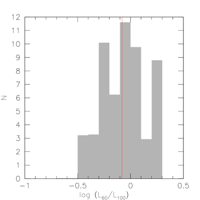
Figure 2: The distribution of the rest–frame luminosity ratio, $\log L_{60}/L_{100}$, for our 56 IDS/ISOCAM sources; red continuous line corresponds to the value $\log L_{60}/L_{100}=-0.08$ (see text).

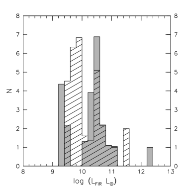
Figure 3: The rest-frame far-infrared luminosity distribution for the IDS/ISOCAM sample of 56 galaxies. The separate distributions of warm (24 sources) and cold (32 sources) sub-populations are indicated with the (grey) open and (white) hatched histograms, respectively.

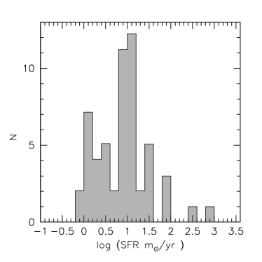
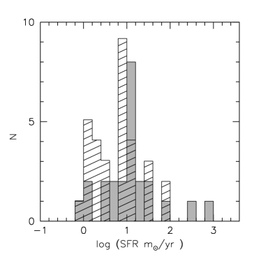
Figure 4: Left: The SFR distribution for our sample of 56 sources. Right: The SFR distribution for warm, 24, and for cold, 32 sources, (grey) open and (white) hatched histogram respectively.

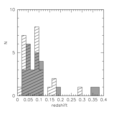
Figure 5: The redshift distribution for warm, 24, and for cold, 32 sources, (grey) open and (white) hatched histogram respectively.

The more luminous 60 $\mu$m sources, i.e., those with higher SFRs, correspond to the more distant systems, 3-96 and 3-53, two warm sources (Fig. 4).

The dust temperatures suggest the presence of two galaxy populations: a spiral population with normal dust temperature (i.e., $<$ 36 K), mean SFR $\simeq 6$ M${}_{\odot}/$yr, mean far-IR luminosity, $\log(L_{FIR})$, $\simeq$ 10.1, and mean redshift 0.075, together with a starburst population characterized by warm dust temperature (i.e., $\geq 36\,$K), mean SFR $\simeq 12$ M${}_{\odot}/$yr, mean far-IR luminosity, $\log(L_{FIR})\simeq 10.3$, and mean redshift 0.1 (Fig. 5).

3 The 60 $\mu$m luminosity function

The observed flux $S_{\nu}$ is related to the rest-frame luminosity by:

$$L_{\nu}=4\pi\,\,D_{L}^{2}\,\,S_{\nu}\,\,/k\left(L,\,z\right)$$ (1)

where $D_{L}$ is the luminosity distance, computed according our cosmological model (§1), and $k\left(L,\,z\right)$ is the $K$-correction defined as:

$$k\left(L,\,z\right)=\frac{\left(1+z\right)\,\,L_{\nu(1+z)}}{L_{\nu}}$$ (2)

For the most distant galaxies ($z>0.2$) the correction exceeds 20% of the luminosity.

Fig.6 shows our derived 60$\,\mu$m differential luminosity function, i.e., the co-moving number density of sources per logarithmic luminosity interval, $\phi(L_{60},z)\Delta$ log$L_{60}$ where $L_{60}=\nu L_{\nu}$, calculated using the Schmidt-Eales $1/V_{max}$ estimator proposed by Schmidt (1968) and improved by Felten (1976) and Eales (1993). We assume Poisson errors, as tabulated by Gehrels (1986). $L_{60}$, i.e., the rest–frame luminosity, has been K–corrected as specified in § 2.

According to the $V/V_{max}$ test Schmidt (1968), sources drawn from a population uniformly distributed in space should have a mean value of $V/V_{max}$ equal to 0.5. Larger (smaller) values of $V/V_{max}$ are the result of a strong increase (decrease) of the co-moving space density of sources with redshift. We find $<V/V_{max}>=0.51\pm 0.06$, consistent with a uniform distribution of sources. The IDS/ISOCAM sample is ten times deeper in flux density than the PSCz catalog and 100 times deeper than the IRAS 60$\mu$m Bright Galaxy Sample Sanders et al. (2003) but no signatures of evolution arise from our sample.

The LF we derive is in good agreement with previous works based on the IRAS PSC Saunders et al. (1990); Takeuchi et al. (2003, 2004). Takeuchi et al. (2003, 2004) revised the work by Saunders et al. (1990) by enlarging their galaxy sample to 15411 galaxies from the PSCz Saunders et al. (2000) with a flux limit of 600 mJy and a redshift range between 0 and 0.07. Their analytic fit, shown as a continuous line in Fig. 6, is based on the same parameterization as Saunders et al. (1990):

$$\phi(L_{\nu})=\phi_{*}\left(\frac{L_{\nu}}{L_{*}}\right)^{1-\alpha}\exp\left[-\frac{1}{2\sigma^{2}}\log_{10}^{2}\left(1+\frac{L_{\nu}}{L_{*}}\right)\right]$$ (3)

with parameters: $\alpha=1.23\pm 0.04$, $L_{*}=(4.34\pm 0.86)\times 10^{8}h^{-2}$ L_⊙, $\sigma=0.724\pm 0.01$, and $\phi_{*}=(2.60\pm 0.30)\times 10^{-2}h^{3}\,$Mpc^-3 Takeuchi et al. (2003, 2004). Our results extend over three orders of magnitude in luminosity, from $\log(L_{60}/L_{\odot})\simeq$ 9 up to more than 12. In the range where the samples overlap our findings agree with the recent determination by Frayer et al. (2006, diamonds in Fig. 6), based on a complete sample of 58 sources with $S_{70}>50$ mJy and $z<0.3$, drawn from the Spitzer extragalactic First Look Survey.
Despite the fact that the redshift range exceeds $z=0.3$, our LF does not show any evidence of evolution.
A more direct test for evolution has been performed by computing LF in four different redshift bins assuming no evolution (see Fig. 6, right panel, and Table 1). The results are fully consistent with this assumption.

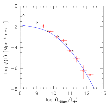
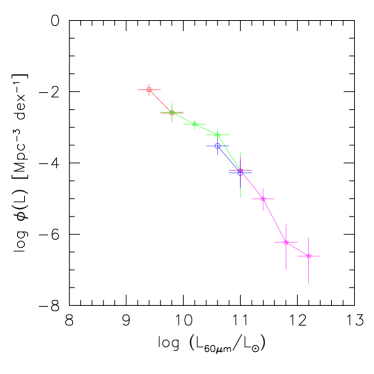
Figure 6: Left:The rest–frame 60 $\mu$m LF for our sample of 56 IDS/ISOCAM sources (red filled squares) compared with LF of IRAS PSCz galaxies from Takeuchi et al. (2003, 2004; blue continuous line) and with LF of Spitzer extragalactic First Look Survey from Frayer et al. (2006) (open diamonds). The bin size is $\Delta\log L_{60}=0.4$. Right: LF split into different redshift bins: asterisks (red) for $z<0.05$, triangles (green) for $0.05\leq z<0.010$, open circles (blue) for $0.010\leq z<0.015$, and stars (magenta) for $z>0.15$.

Table 1: $60\,\mu$m luminosity function: V/V_max in different redshift bins.

redshift bin	V/Vmax
0.00$\leq z<$ 0.05	0.490$\pm$ 0.04
0.05$\leq z<$ 0.10	0.471$\pm$ 0.08
0.10$\leq z<$ 0.15	0.444$\pm$ 0.07
$z>$ 0.15	0.315$\pm$ 0.08

4 The 15$\mu$m luminosity function

Deep surveys at 15$\mu$m carried out using ISO (i.e., Elbaz et al., 1999; Flores, 1999; Lari et al., 2001; Metcalfe et al., 2003) seem to require strong evolution of 15$\mu$m sources starting from redshift 0.5 (see Lagache et al. (2005) and references therein). Several evolutionary models were developed to explain these results (e.g., Franceschini et al., 2001; Rowan-Robinson, 2001) trying to fit IR/submillimiter source counts with different degrees of success. Nevertheless none of them is based on a local LF obtained from 15$\mu$m data, since the only available data until few years ago came from IRAS 12$\mu$m photometry (Rush et al., 1993; Xu, 1998; Fang et al., 1998).

A first attempt to build up the 15$\mu$m LF of a NEPR subsample was made by Xu (2000) using the bi-variate method to translate the 60$\mu$m local LF of IRAS galaxies (Saunders et al., 1990) to 15$\mu$m. Its sample comprises 64 sources detected both at 60$\mu$m Hacking & Houck (1987) and at 15$\mu$m Aussel et al. (2000), with redshifts measured by Ashby et al. (1996). Xu fitted the result obtained (see its Table 2 and Fig. 3), with a pure luminosity evolution model $L\propto(1+z)^{4.5}$. Nevertheless he said that it must be considered as a preliminary work as discussed in § 1.

A recent determination of the 15$\mu$m local LF was made by Pozzi et al. (2004) using the available data on the southern fields, S1 and S2, of the ELAIS survey Oliver et al. (2000). Their data sample entails 150 galaxies with redshift $z\leq 0.4$, excluding sources classified as AGNs (both type one and type two). The 15$\mu$m LF was calculated with a parametric maximum likelihood method. Pozzi et al. (2004) separate spirals from starbursts using optical/mid-IR ratios, assuming that Starbursts are the more mid-IR luminous galaxies with, on average, larger $\log(L_{15}/L_{R}$) ratios. They estimate the 15$\mu$m local LF in the range $7.8\leq\log(L/L_{\odot})\leq 10.6$. Their findings are that the 15$\mu$m LF of spirals is consistent with no evolution, ($<V/V_{\mathrm{max}}>=0.55\pm 0.03$), but that the value $<V/V_{\mathrm{max}}>=0.64\pm 0.03$ measured for the starbursts suggests that this population is in fact evolving.

4.1 The bi-variate method

Since our sample is flux limited at 60$\mu$m, but not at 15$\mu$m, we used the bi-variate method to calculate the 15$\mu$m LF of our sample. It was obtained by a convolution of the 60$\mu$m LF with the log($L_{15}/L_{60}$) distribution:

$$\phi(\log L_{15})=\int\phi(\log L_{60})\,P(\log(L_{15}/L_{60}))\,d(\log L_{60})$$ (4)

where $P(log(L_{15}/L_{60}))$ is the conditional probability function that gives the distribution of log($L_{15}$) around the mean 15$\mu$m luminosity $\langle log(L_{15})\rangle$ at a given 60$\mu$m luminosity log($L_{60}$).

The distribution per unit interval of the logarithm of the luminosity ratio is well described by Type I Pearson’s curves (Pearson, 1924; Elderton & Johnson, 1969):

$$y=y_{0}\,\,(1+x/a_{1})^{m1}\,\,(1-x/a_{2})^{m2}$$ (5)

where $x=\log(L_{15}/L_{60})$, with $-a_{1}\leq x\leq a_{2}$, and origin at the position of the peak of the distribution (mode). The values of the parameters are given in Table 2, together with the mean, the standard deviation $\sigma$, the skewness ($\mu_{3}^{2}/\mu_{2}^{3}$) and the kurtosis ($\mu_{4}/\mu_{2}^{2}-3$) of the distribution ($\mu_{i}$ is the $i$-th moment about the mean). The quality of the fit is quantified by the value of $\chi^{2}$ per degree of freedom ($\chi_{\nu}$), given in the last column and computed adopting the Levenberg-Marquardt method as implemented in Press et al. (1992); $\sigma_{p}$ are the errors on the Pearson’s parameters.

To perform these analyses we remove from our sample the sources 3-70 and 3-96 with AGN properties (see § 2) and used the parametric solution of the 60$\mu$m LF derived by Takeuchi et al. (2003, 2004), which agrees well with our results (see § 3, eq. 3).

Table 2: Coefficients and parameters describing the distribution function, Pearson I curve of our sample.

Case	$y_{0}$	$a_{1}$	$a_{2}$	$m_{1}$	$m_{2}$	Mode	Mean	$\sigma$	Skew	Kurt	$\chi_{\nu}^{2}$
All	82.8	12.9	0.43	83.3	2.72	-0.60	-0.69	0.24	0.52	0.52	0.77
$\sigma_{p}$	16.5	1.56	0.04	10.2	0.39	0.04

Table 3: Parameters describing the LF of our sample.

Case	$\phi_{*}/10^{-3}\,Mpc^{-3}$	$L_{*}/10{{}^{8}}\,L_{\odot}$	$\phantom{)))))}\alpha$	$\phantom{)))))}\sigma$
All	$5.32\pm.40$	$2.00\pm.18$	$1.241\pm.021$	$0.748\pm.010$

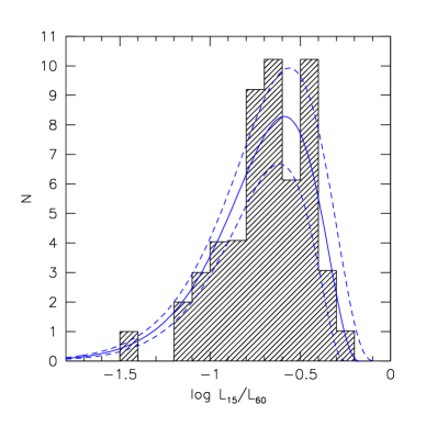
Figure 7: Distribution of the $\log L_{15}/L_{60}$ ratio for 54 IDS/ISOCAM sources (see text). The bin size is $\Delta(\log L_{15}/L_{60})=0.1$. The fitting function is a Type I Pearson whose parameters, optimized following the Levenberg-Marquardt method (see text), are reported in Table 2; dashed lines show the same curves with 1$\sigma$ error in the parameters.

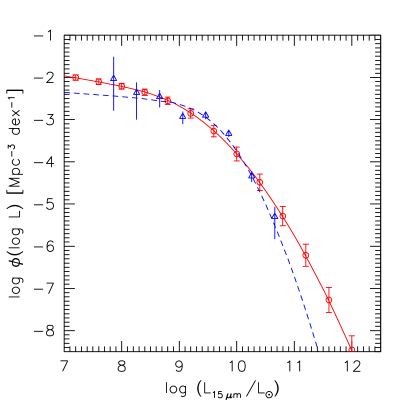
Figure 8: The 15$\,\mu$m differential LF (red continuous line) for the IDS/ISOCAM sample (54 sources) compared with that of Pozzi et al. (2004) (blue dashed line and open triangles). The error bars correspond to one $\sigma$ error of the Pearson’s curve parameters.

Table 3 lists the parameters defining our 15 $\mu$m local galaxy LF using the same parametric form as in eq. (3) suggested by Pozzi et al. (2004). The Pozzi LF extends from 7.8 up to 10.6 in log(L${}_{15}/$L${}_{\odot})$, whereas our convolution extends over more than six orders of magnitude and 100 times deeper (Fig. 8). Our results agree with those by Pozzi et al. (2004) up to their luminosity limit (10.6), however, beyond such a luminosity the two parametric LFs diverge so that at log(L${}_{15}/$L_⊙)=11 we expect 10 times more sources than Pozzi et al. (2004).

4.2 Spiral and starburst populations

Our sample includes 22 galaxies with rest-frame warm $L_{60}/$L₁₀₀ ratios and 32 galaxies with cold ratios after excluding AGN (see § 2). They define two different populations, starburst and spiral galaxies respectively, as far as dust properties are concerned. Their distributions per unit interval of the logarithm of the luminosity ratios $\log(L_{15}/L_{60}$), shown in Fig. 9 (left panel), are fitted well by Pearson’s curves whose parameters are in Table 4. Their 15 $\mu$m LF fits, i.e., eq. (3), are in Fig. 9 (right panel) and the LF parameters are given in Table 5. We find that both populations contribute to the faint end of the LF. Spiral galaxies overcome starbursts by less than a factor of two. Such a factor is slightly reducing with luminosity, from 1.8 at $\log(L_{15}/L_{\odot})=8$ to 1.3 at $\log(L_{15}/L_{\odot}=11.8)$. Our results differ from those of Pozzi et al.(2004), in particular predictions concerning starburst population. However they used optical/mid-IR ratios instead of far-IR ratios to disentangle starbursts and spirals, assuming that starbursts are the more mid-IR luminous galaxies with, on average, larger $\log(L_{15}/L_{R}$) ratios.

Table 4: Coefficients and parameters describing the distribution function, Pearson I curve, of starburst and spiral populations.

Case	$y_{0}$	$a_{1}$	$a_{2}$	$m_{1}$	$m_{2}$	Mode	Mean	$\sigma$	Skew	Kurt	$\chi_{\nu}^{2}$
Starbursts	35.7	4.30	0.14	9.11	0.25	-0.39	-0.70	0.25	1.99	2.39	1.70
$\sigma_{p}$	12.3	1.55	0.02	3.56	0.18	0.002
Spirals	43.2	1.47	0.32	4.43	0.19	-0.64	-0.64	0.23	0.05	-0.84	0.77
$\sigma_{p}$	11.6	0.58	0.01	1.89	0.11	0.01

Table 5: Parameters describing the LF of starburst and spiral populations.

Case	$\phi_{*}/10^{-3}\,Mpc^{-3}$	$L_{*}/10{{}^{8}}\,L_{\odot}$	$\phantom{)))))}\alpha$	$\phantom{)))))}\sigma$
Starbursts	$1.89\pm.03$	$2.96\pm.03$	$1.275\pm.001$	$0.740\pm.015$
Spirals	$3.36\pm.07$	$2.21\pm.07$	$1.236\pm.006$	$0.739\pm.027$

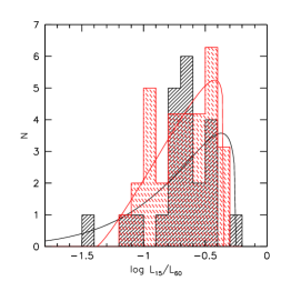
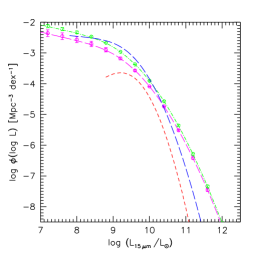
Figure 9: Left: Distribution of the $\log L_{15}/L_{60}$ ratios for starbursts (black continuous line), 22 sources, and spirals (red dashed line) 32, sources, selected on the basis of their far-IR colors. The bin size is $\Delta(\log L_{15}/L_{60})=0.1$ and the parameters of the fitting functions, Type I Pearson curves, are in Table 4 together with one $\sigma$ errors. Right: The contribution of such galaxy populations to the rest-frame 15$\mu$m LF (see Table 5): starbursts (magenta long–dashed dotted line) and spirals (green dot-dashed line). Results are compared with those by Pozzi et al. (2004): starbursts (red short–dashed line) and spirals (blue long-dashed line).

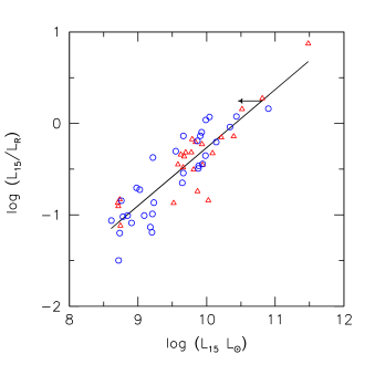
Figure 10: The behavior of the $\log L_{15}/L_{R}$ ratio for warm sources (24, red triangles), and for cold sources (32, blue open circles) of IDS/ISOCAM sample; the continuous line corresponds to the least–square fit (see eq. 6).

To investigate further this point, we repeated our analysis using the same criterion of Pozzi et al. to discriminate starbursts from spirals. We used APS catalog (http://aps.umn.edu) R-band magnitudes for the 37.5% of our sample galaxies that lacked them (see § 1), applying a correction of -0.75 magnitudes to bring the APS zeropoint into agreement with our own common sources.

Fig. 10 shows the rest–frame $L_{15}/L_{R}$ ratios vs. $L_{15}$ luminosity. From a least–square–fitting procedure we find:

$$L_{15}/L_{R}=(0.64\pm 0.04)\times L_{15}-(6.67\pm 0.43)$$
(6)

with a dispersion of 0.20 dex. Our fit is steeper, 0.64 instead of 0.5, than that of Pozzi et al. (2004). Following Pozzi et al. (2004), we assume $L_{15}/L_{R}=-0.4$ as the nominal separation between spiral and starburst populations. Warm and cold galaxies, selected on the basis of their far–IR colors, are mixed in Fig. 10. Such a criterion selects different galaxies in both the populations. Now there are 30 spirals and 24 starbursts in our sample. The distributions per unit interval of the logarithm of their luminosity ratios $\log(L_{15}/L_{60}$), are fitted again by Type I Pearson’s curves (Fig. 11, left panel) whose parameters are in Table 6. Table 7 shows those of their 15 $\mu$m LF fits (Fig. 11, right panel).

Table 6: Coefficients and parameters describing the distribution functions, Pearson I curves, of starburst and spiral populations.

Case	$y_{0}$	$a_{1}$	$a_{2}$	$m_{1}$	$m_{2}$	Mode	Mean	$\sigma$	Skew	Kurt	$\chi_{\nu}^{2}$
Starbursts	35.11	11.5	0.62	61.2	3.45	-0.63	-0.74	0.29	0.50	0.56	0.86
$\sigma_{p}$	10.7	2.29	0.12	12.3	0.74	0.11
Spirals	60.3	10.0	0.33	47.8	0.94	-0.60	-0.67	0.21	0.41	-0.34	1.03
$\sigma_{p}$	13.0	2.61	0.13	12.6	0.47	0.11

Table 7: Parameters describing the LF of starburst and spiral populations.

Case	$\phi_{*}/10^{-3}\,Mpc^{-3}$	$L_{*}/10{{}^{8}}\,L_{\odot}$	$\phantom{)))))}\alpha$	$\phantom{)))))}\sigma$
Starbursts	$3.82\pm.62$	$1.81\pm.45$	$1.245\pm.048$	$0.761\pm.028$
Spirals	$2.92\pm.88$	$2.29\pm.85$	$1.234\pm.084$	$0.742\pm.037$

Both such populations contribute to the faint end of the LF. The space densities of starbursts are just slightly greater than those of spiral galaxies.

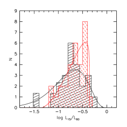
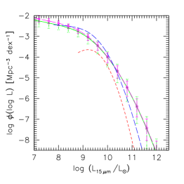
Figure 11: Left: The distribution of the $\log L_{15}/L_{60}$ ratio for starbursts (black continuous line), 24 sources, and for spirals (red dashed line) 30 sources, selected with the same criterion as Pozzi et al. (2004). The bin sizes are $\Delta(\log L_{15}/L_{60})=0.12$ and 0.1 respectively. The parameters of the fitting functions, Type I Pearson curves, are in Table 6. Right: The contribution of such galaxy populations to the rest-frame 15$\mu$m LF (see Table 7): starbursts (magenta long–dashed dotted line) and spirals (green dot–dashed line). Our results are compared with those by Pozzi et al. (2004): starbursts (red short–dashed line) and spirals (blue long-dashed line).

5 Conclusions

Combining our observations della Valle et al. (2006) with those by Ashby et al. (1996) we have reliable identifications and spectroscopic redshifts for 100% of the complete far–IR selected subsample comprising 56 IDS sources with $S_{60}>80$mJy Mazzei et al. (2001). The redshift distribution shows a tail extending up to $z\simeq 0.37$, in particular $\simeq$ 26% of the sources have redshifts $z>0.1$.

To fully exploit the potential of this sample, ten times deeper than the IRAS PSC, thus less liable to the effect of local density inhomogeneity, for investigating galaxy evolution, we calculate the 60$\mu$m LF using the $1/V_{max}$ method. Current estimates are based on rather shallow samples. Even though our sample is five times deeper in redshift than the PSCz Saunders et al. (2000) used by Takeuchi et al. (2003), our LF agree with their determination Takeuchi et al. (2003, 2004) and with that by Frayer et al. (2006) based on a complete sample of galaxies with $S_{70}>50$ mJy drawn from the Spitzer extragalactic First Look Survey. Despite the fact that our redshift range exceeds $z=0.3$, and our 60$\mu$m LF extends up to $\log L_{60}=12$, whereas that by Frayer et al.(2006) up to $\log L_{60}\simeq 11$, it does not show any evidence of evolution. The $V/V_{max}$ test gives a value consistent with an uniform distribution ($V/V_{max}=0.51\pm 0.06$). Moreover, a more direct test for evolution has been performed by splitting the LF in different redshift bins assuming no evolution. The results are fully consistent with this assumption.

We present the bi-variate 15$\mu$m LF, one of the few determinations based on ISO data, by convolving the 60$\mu$m LF with the luminosity ratio distribution, $L_{15}/L_{60}$ of our sample. This extends to luminosity 100 times higher than before. Our result agrees with the recent determination by Pozzi et al. (2004) in the common range of luminosity, i.e., from 7.8 up to 10.6 in $\log(L_{15}/L_{\odot})$. However, above $\log(L_{15}/L_{\odot})=10.6$, the two parametric LFs diverge so that at $\log(L_{15}/L_{\odot})=11$ we expect 10 times more sources than Pozzi et al. (2004).

In order to investigate the role of galaxy populations on such a result, we disentangle starbursts and spirals on the basis both of their far-IR dust temperature, and of their $L_{15}/L_{R}$ ratios, as assumed by Pozzi et al. (2004). Such criteria select galaxies with different dust properties, as we point out in § 4.2. Nevertheless, we find that both galaxy populations contribute to the faint end of the rest-frame 15$\mu$m LF, even though we adopt the same criterion as Pozzi et al. (2004). Moreover, in this case, above $\log(L_{15}/L_{\odot})=9$ our findings are that starbursts and spirals give almost the same contribution to the mid–IR LF whereas Pozzi et al. (2004) predict that spirals contribute 5-10 times more than starbursts.