Modeling Integrated Properties and the Polarization of the Sunyaev-Zeldovich Effect

Abstract

Two little explored aspects of Compton scattering of the CMB in clusters are discussed: The statistical properties of the Sunyaev-Zeldovich (S-Z) effect in the context of a non-Gaussian density fluctuation field, and the polarization patterns in a hydrodynamcially-simulated cluster. We have calculated and compared the power spectrum and cluster number counts predicted within the framework of two density fields that yield different cluster mass functions at high redshifts. This is done for the usual Press & Schechter mass function, which is based on a Gaussian density fluctuation field, and for a mass function based on a $\chi^{2}$-distributed density field. We quantify the significant differences in the respective integrated S-Z observables in these two models.

S-Z polarization levels and patterns strongly depend on the non-uniform distributions of intracluster gas and on peculiar and internal velocities. We have therefore calculated the patterns of two polarization components that are produced when the CMB is doubly scattered in a simulated cluster. These are found to be very different than the patterns calculated based on spherical clusters with uniform structure and simplified gas distribution.

1 Introduction

The pioneering experimental and observational CMB work of our esteemed colleague Francesco Melchiorri has paved the way for generations of students and colleagues in Italy and elsewhere, who are continuing the mission he helped define and lead for more than 30 years. Francesco worked hard to advance experimental and observational capabilities to measure the Sunyaev-Zeldovich (S-Z) effect in nearby clusters. His expertise and leadership resulted in the successful development of MITO, the measurement of the effect in the Coma cluster (De Petris et al. 2002), and the upgrading of MITO to a bolometer array (Lamagna et al. 2005). As noted by Rephaeli (2005) in Francesco’s obituary, his passing marks the end of the founder’s era in the growth of the thriving Italian CMB community.

In light of current and future capabilities of the many upcoming S-Z experiments, we have calculated the power spectrum and cluster number counts in the context of a specific non-Gaussian density fluctuation field. As we discuss in the next section, certain observational results point to the possible need for excess power on cluster scales. The enhanced interest in non-Gaussian models motivates contrasting the integrated S-Z observables of one such viable model with those of the standard Gaussian model whose parameters are well determined.

Future sensitive mapping of the S-Z effect in individual clusters will allow measuring its polarization level. A basic description of some of the S-Z polarization patterns in clusters has already been given by Sazonov & Sunyaev (1999). In Section 3 we briefly summarize some of the features of two of the polarization components that are induced when the CMB is doubly scattered in a (non-idealized) cluster whose dynamical state and gas properties are deduced directly from hydrodynamical simulations.

2 Integrated S-Z Observables in a Non-Gaussian Model

It has been suggested (Mathis, Diego, & Silk 2004) that some observational results possibly point to an appreciable deviation from a Gaussian probability distribution function (PDF) of the primordial density fluctuation field. These are the relatively high CMB power at high multipoles measured by the CBI (Mason et al. 2003) and ACBAR (Kuo et al. 2004) experiments, the detection of structures with high velocity dispersions at redshifts $z=4.1$ (Miley et al. 2004) and $z=2.1$ (Kurk et al. 2004), and the apparent slow evolution of the X-ray luminosity function (as deduced from catalogs compiled by Vikhlinin et al. 1998 and Mullis et al. 2003).

Analyses of WMAP all-sky maps (Komatsu et al. 2003, McEwen et al. 2006) do not rule out an appreciable non-Gaussian PDF tail on clusters scales. Enhanced power on the scales of clusters may lead to detectable differences in S-Z power levels and cluster number counts as compared with those predicted from the standard Gaussian PDF. It is of interest, therefore, to explore the consequences of a non-Gaussian PDF, especially in light of the large S-Z surveys that will be conducted by ground-based telescopes and the Planck satellite. These will measure the effect in thousands of clusters and map the anisotropy it induces in the CMB spatial structure.

The non-Gaussian model we consider here has its origin in isocurvature fluctuations produced by massive scalar fields that are thought to have been present during inflation. The model is characterized by a PDF that has a $\chi^{2}_{m}$ distribution of $m$ CDM fields which are added in quadratures (Peebles 1997, 1999, Koyama, Soda & Taruya 1999).

We have carried out detailed calculations of the S-Z power spectrum and cluster number counts predicted in the standard Gaussian and a non-Gaussian model with $m=1,2$. Below we briefly describe the principal aspects of our work and its main results; a more comprehensive description can be found in Sadeh, Rephaeli & Silk (2006; hereafter, SRS).

2.1 Calculations

The integrated statistical properties of the population of clusters involve the basic cosmological and large-scale quantities, and essential properties of intracluster (IC) gas. For Gaussian models these properties have been quantitatively determined by semi-analytic calculations (e.g., Kaiser 1981, Colafrancesco et al. 1994, 1997, Molnar & Birkinshaw 2000, Sadeh & Rephaeli 2004) and from hydrodynamical simulations (e.g., Springel et al. 2001).

The Press & Schechter (1974) mass function is

$$n(M,z)=-F(\mu)\frac{\rho_{b}}{M\sigma}\frac{d\sigma}{dM}dM,$$ (1)

where $\mu\equiv\delta_{c}/\sigma$ and $\rho_{b}$ is the background density. The critical overdensity for spherical collapse (which is only weakly dependent on redshift) is assumed to be constant, $\delta_{c}=1.69$, and the density field variance, smoothed over a top-hat window function of radius $R$, is

$$\sigma^{2}(R)=\int_{0}^{\infty}P(k)\widetilde{W}^{2}(kR)k^{2}dk,$$ (2)

where $P(k)\equiv Ak^{n}T^{2}(k)$. Evolution of the mass variance is given in

$$\sigma(M,z)=\frac{g[\Omega_{m}(z)]}{g[\Omega_{m}(0)]}\frac{\sigma(M,0)}{1+z},$$ (3)

where

$$\Omega_{m}(z)=\frac{\Omega_{m}(0)(1+z)^{3}}{(1+z)^{2}[1+\Omega_{m}(0)z-\Omega_{\Lambda}(0)]};\,\,\,\Omega_{\Lambda}(z)=1-\Omega_{m}(z),$$ (4)

and (Carroll, Press & Turner 1992)

$$g[\Omega_{m}(z)]=\frac{2.5\Omega_{m}(z)}{[\Omega_{m}(z)^{4/7}-\Omega_{\Lambda}+(1+\Omega_{m}(z)/2)(1+\Omega_{\Lambda}/70)]}.$$ (5)

The function $F(\mu)$ in equation (1) assumes the form

$$F(\mu)=\sqrt{\frac{2}{\pi}}\displaystyle{e^{-\frac{\mu^{2}}{2}}}\frac{\mu}{\sigma_{R}},$$ (6)

for a Gaussian density field, and the form

$$F(\mu)=\frac{\left(1+\sqrt{\frac{2}{m}}\mu\right)^{m/2-1}}{(\frac{2}{m})^{(m-1)/2}\Gamma{(\frac{m}{2})}}e^{\left[-\frac{m}{2}\left(1+\sqrt{\frac{m}{2}}\mu\right)\right]}\frac{\mu}{\sigma_{R}},$$ (7)

for a density fluctuation field which is distributed according to the $\chi^{2}_{m}$ model mentioned above.

The highest contrast with the standard model is obtained for $m=1$, the case we have mostly explored and discuss here, but in order to demonstrate the impact of this parameter on PDF tail, we have also considered the case $m=2$ (for details, see SRS). Note that the higher the value of $m$, the closer is the PDF to a Gaussian, as would be expected from the central limit theorem.

The CDM transfer function for the Gaussian model is

$$T(k)=\frac{\ln{(1+2.34q)}}{2.34q}[1+3.89q+(16.1q)^{2}+(5.46q)^{3}+(6.71q)^{4}]^{-1/4}.$$ (8)

For the the $\chi^{2}_{m}$ model, we adopt the isocurvature CDM transfer function

$$T(k)_{iso}=(5.6q)^{2}\left[1+\frac{(40q)^{2}}{1+215q+(16q)^{2}/(1+0.5q)}+(5.6q)^{8/5}\right]^{-5/4},$$ (9)

with $q\equiv k/(\Omega_{m}h^{2})\,Mpc^{-1}$ (Bardeen et al. 1986). We adopt the (now) standard $\Lambda$CDM flat cosmological model, with $\Omega_{\Lambda}=0.7$, $\Omega_{m}=0.3$, $h=0.7$. In the Gaussian case the spectral index was taken to be $n=1$ with mass variance normalization $\sigma_{8}=0.9$. In the non-Gaussian model $n=-1.8$, and by requiring that the present cluster abundance is the same as calculated in the Gaussian model, the value $\sigma_{8}=0.73$ was deduced the $\chi^{2}_{1}$ model.

The basic expression in the calculation of the S-Z angular power spectrum is

$$C_{\ell}=\int_{z}\,r^{2}\frac{dr}{dz}\int_{M}n(M,z)\,G_{\ell}(M,z)\,dM\,dz,$$ (10)

where $r$ is the co-moving radial distance, and $G_{\ell}$ is obtained from the angular Fourier transform of the profile of the thermal S-Z temperature change at an angular distance $\theta$ from the center of a cluster, , $\Delta T(\theta)$. The function $G_{\ell}$, which is proportional to $(\Delta T)^{2}$, is fully specified in, e.g., Molnar & Birkinshaw (2000). In the limit of non-relativistic electron velocities the relative temperature change assumes the simple form

$$\frac{\Delta T}{T}(\theta)=\left[x\coth{\left(\frac{x}{2}\right)}-4\right]y(\theta).$$ (11)

For an isothermal cluster with a $\beta$ density profile, the Comptonization parameter is

$$y(\theta)=\frac{2k_{B}\sigma_{T}}{m_{e}c^{2}}\frac{n_{0}(M,z)T_{0}(M,z)r_{c}(M,z)}{\sqrt{1+(\theta/\theta_{c})^{2}}}\tan^{-1}\left[p\sqrt{\frac{1-(\theta/p\theta_{c})^{2}}{1+(\theta/\theta_{c})^{2}}}\right],$$ (12)

where $n_{0}$, $T_{0}$, are the central electron density, temperature, and $r_{c}$, and $\theta_{c}$ are the core radius and the angle subtended by the core, respectively. The gas profile is truncated at an outer radius $R=10r_{c}$.

The mass-temperature scaling relation is of basic importance for relating the magnitude of the S-Z effect to the cluster mass, and thereby to the mass function. We have used the following form for this relation

$$T(M,z)=T_{15}\left(\frac{M}{10^{15}h^{-1}M_{\odot}}\right)^{\alpha}(1+z)^{\psi},$$ (13)

normalized such that the gas temperature of a $10^{15}h^{-1}M_{\odot}$ cluster is $8.5\,keV$ (at $z=0$). The parameter $\alpha$ is usually taken to be $2/3$, in accordance with theoretical predictions based on hydrostatic equilibrium; we use a range of values that $\pm 10\%$ around $2/3$. The uncertainty in the evolution of the gas temperature is accounted for by taking the two extreme values of $0$ and $1$ for the parameter $\psi$, signifying either no evolution, or strong evolution, respectively.

The electron density is

$$n_{e}(M,z)\simeq n_{0}\frac{f}{0.1}(1+z)^{3},$$ (14)

with the scaling of the gas mass fraction to $\sim 10\%$ (e.g. , Carlstrom, Holder & Reese 2002). Since we do not yet know the redshift dependence of $f$, we assume $f=0.1$ to be roughly valid throughout the redshift interval ($0-6$) considered here. Finally, the core radius is calibrated according to the simple relation

$$r_{c}=0.15h^{-1}\,\left(\frac{M}{10^{15}h^{-1}M_{\odot}}\right)^{1/3}\frac{1}{1+z}\,Mpc.$$ (15)

Observations indicate a variance of $\sim 20\%$ in the value of the core radius, which is assumed here, with a corresponding range in the value of the central density.

The number of clusters with S-Z flux (change) above $\Delta\overline{F}_{\nu}$ is (e.g. Colafrancesco et al. 1997)

$$N(>\Delta\overline{F}_{\nu})=\int r^{2}\frac{dr}{dz}dz\int_{\Delta\overline{F}_{\nu}}n(M,z)\,dM.$$ (16)

For a cluster with mass M at redshift z

$$\Delta F_{\nu}=\displaystyle\frac{2(k_{B}T)^{3}}{(hc)^{2}}g(x)y_{0}\int R_{s}(|\hat{\gamma}-\hat{\gamma_{\ell}}|,\sigma_{B})\cdot y(|\hat{\gamma_{\ell}}|,M,z)\,d\Omega,$$ (17)

where $\hat{\gamma_{\ell}}$ and $\hat{\gamma}$ denote line of sight (los) directions through the cluster center, and relative to this central los, respectively,

$$y_{0}=2\frac{k_{B}\sigma_{T}}{m_{e}c^{2}}n_{0}(M,z)T_{0}(M,z)r_{c}(M,z),$$ (18)

and the spectral dependence (of the thermal component) of the effect is given (in the nonrelativistic  limit; more on this later in this section) by

$$g(x)\equiv\frac{x^{4}e^{x}}{(e^{x}-1)^{2}}\left[x\coth{(x/2)-4}\right],$$ (19)

where $x=h\nu/kT$. The profile of the effect is given in

$$y(|\hat{\gamma_{\ell}}|,M,z)\equiv\displaystyle\frac{1}{\sqrt{1+(\theta/\theta_{c})^{2}}}\cdot\tan^{-1}{\left[p\sqrt{\frac{1-(\theta/p\theta_{c})^{2}}{1+(\theta/\theta_{c})^{2}}}\right]},$$ (20)

which is the los integral along a direction that forms an angle $\theta$ with the cluster center. $R_{s}(|\hat{\gamma}-\hat{\gamma_{\ell}}|,\sigma_{B})$ denotes the angular response of a detector whose beam size is given in terms of $\sigma_{B}$. Finally,

$$\Delta\overline{F}_{\nu}=\displaystyle\frac{\int\Delta F_{\nu}E(\nu)d\nu}{\int E(\nu)d\nu},$$ (21)

is the flux weighted over the detector spectral response $E(\nu)$.

For determining S-Z cluster number counts we adopt the PLANCK/HFI detection limit of $30\,mJy$. This flux limit translates to a lower limit of the integral over the mass function, equation (16). The results for the S-Z power spectrum and number counts described below refer to these two models: (a) IC gas temperature evolves with time according to $\psi=1$, and (b) no temperature evolution, $\psi=0$. Power spectra were calculated at $\nu=353$ GHz, with a $7.1^{\prime}$ beam size. Number counts were calculated also at $\nu=143$ GHz and $\nu=545$ GHz.

2.2 Results

The augmented tail of the non-Gaussian distribution function (compared with that of a Gaussian) leads to earlier cluster formation (by virtue of the higher probability that an overdense region attains the critical density for collapse) and enhanced high-mass cluster abundance. Thus, in the non-Gaussian case the S-Z power spectrum reaches higher levels, and its peak shifts to higher multipoles, reflecting the higher density of distant clusters. This effect is greatly reduced in a non-evolving temperature model (in which the $1+z$ scaling is factored out).

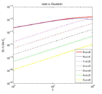
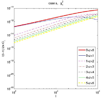
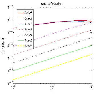
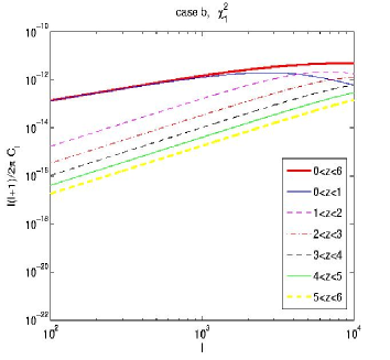
Figure 1: Power spectrum of the S-Z effect. Shown are levels of power contributed by clusters in the redshift range of $0<z<6$, and at 6 redshift intervals. Left and right-hand panels correspond to the Gaussian and $\chi^{2}_{1}$ models, respectively. Upper and lower panels relate to cases (a) and (b), respectively

.

Power spectra calculated over the redshift interval $[0,6]$ for cases (a) and (b) are plotted in Fig. 1 and Fig. 2. In these figures the upper and lower panels correspond to cases (a) and (b), and the left and right panels are for the Gaussian and $\chi^{2}_{1}$ models, respectively. The figures show the distribution of the power spectrum with redshift (Fig. 1) in $\Delta z=1$ and in (logarithmic) mass intervals of $\log{\Delta M}=1$ (Fig. 2), respectively. The maximum power levels attained in case (a) are $\sim 3\cdot 10^{-12}$ and $\sim 6\cdot 10^{-11}$ for the Gaussian and non-Gaussian models, respectively. Both spectra peak at multipoles higher than $\ell>10,000$; in the Gaussian model this is due to the high gas densities of distant clusters, whereas in the non-Gaussian model this behavior is attributed to the combination of high gas densities and the long high-mass tail.

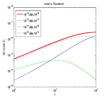
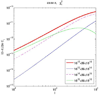
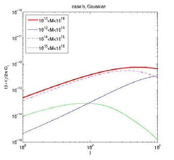
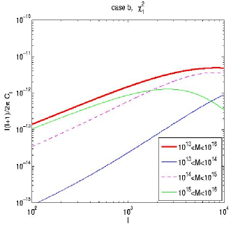
Figure 2: As in the previous figure, but here levels of the power spectra are calculated for four mass intervals spanning the range $10^{13}h^{-1}M_{\odot}<M<10^{16}h^{-1}M_{\odot}$.

Distant clusters are cooler in case (b) than in case (a), due to the redshift independence of their temperatures, so that power levels are lower ($\sim 8\cdot 10^{-13}$ and $5\cdot 10^{-12}$) in the Gaussian and $\chi^{2}$ models, respectively. In the Gaussian model the power peaks at $\ell\sim 6000$, reflecting the lower contribution from cooler, more distant clusters. In the non-Gaussian model, a relatively high abundance of massive clusters at high redshifts leads to sustained high power levels on these scales. Note that irrespective of whether or not the temperature changes with redshift, it still increases with increasing mass, so even when $\psi=0$ a more abundant population of hot clusters is present in the $\chi^{2}$ model. In the $\chi^{2}$ model the contribution of relatively high $z$ clusters to the power is quite evident; in case (a) the contribution of clusters lying in the redshift range $0<z<1$ peaks at $\ell\sim 3000$, but the total power continues to rise due mostly to clusters in the range $1<z<2$. The same behavior, though less pronounced, is evident in case (b).

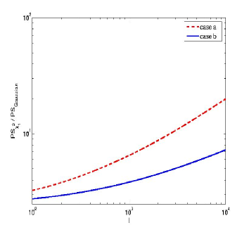
Figure 3: A comparison of S-Z power spectrum levels in the $\chi^{2}_{1}$ and Gaussian models for cases (a) and (b).

The distribution of S-Z power in four mass intervals is plotted in Fig. 2. Of course, the highest mass interval ($10^{15}h^{-1}M_{\odot}<M<10^{16}h^{-1}M_{\odot}$ is most significant in distinguishing between the signatures of Gaussian and non-Gaussian models. Clusters with masses in this range contribute negligibly at all multipoles in the Gaussian model (for which most of the power is produced by clusters in the mass range $10^{14}h^{-1}M_{\odot}<M<10^{15}h^{-1}M_{\odot}$), whereas they dominate the total power up to $\ell\sim 1000$ and $\ell\sim 2000$ in cases (a) and (b), respectively. At higher multipoles the $10^{14}h^{-1}M_{\odot}<M<10^{15}h^{-1}M_{\odot}$ range dominates. In the Gaussian model the contribution of low-mass clusters in the range $10^{13}h^{-1}M_{\odot}<M<10^{14}h^{-1}M_{\odot}$ is dominant only at the highest multipoles. To contrast the predictions of the two models, the ratio of total level of the S-Z power in the $\chi^{2}_{1}$ model to that in the Gaussian model for cases (a) and (b) is shown in Fig. 3. For $\ell=10^{3}-10^{4}$, this ratio increases from $7$ to $20$ in case (a), and from $\sim 4$ to $\sim 7$ in case (b).

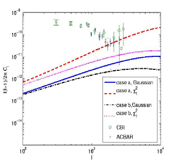
Figure 4: Predicted S-Z power spectra at 31 GHz together with CBI and ACBAR datapoints.

Perhaps the strongest motivation for a non-Gaussian PDF is the apparent difficulty in interpreting the power measured at high $\ell$ by CBI (Mason et al. 2003) and ACBAR (Kuo et al. 2004) as (mostly) S-Z induced anisotropy in a Gaussian model. The predicted power spectra in the Gaussian and $\chi^{2}_{1}$ models are shown in Fig. (4) together with the CBI and ACBAR measurements. The results of the calculations were appropriately adjusted to 31 GHz, the observation frequency of CBI. It seems difficult to reconcile the Gaussian results with the data, while the predicted S-Z power in case (a) of the $\chi^{2}_{1}$ model matches reasonably well the observed power ‘excess’ (over the extrapolated power measured by WMAP) at $\ell\geq 2000$ (see also Mathis et al. 2004).

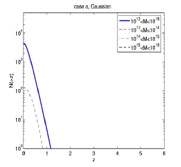
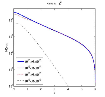
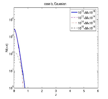
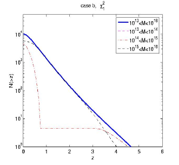
Figure 5: Cumulative S-Z counts as function of redshift in four mass intervals. (The contribution from the lowest mass interval, $10^{13}<M<10^{14}\,M_{\odot}$ , vanishes in all the cases considered here.

A more direct manifestation of the enhanced high-mass non-Gaussian PDF is apparent in the higher (cumulative) counts in this model, and a redshift distribution that is different than in the Gaussian model. In Fig. 5 we show the redshift distribution of cumulative S-Z number counts. The plots are arranged by the specific model (as in Fig. 1 and Fig. 2). Note that in all models considered here only clusters with masses higher than $10^{14}h^{-1}M_{\odot}$ generate fluxes that exceed the adopted detection limit of $30\,mJy$.

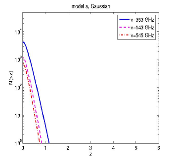
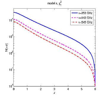
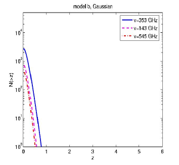
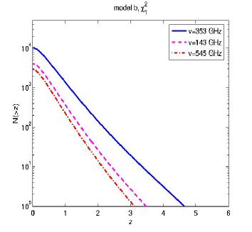
Figure 6: Cumulative S-Z counts as a function of redshift. Number counts are shown for the three specified frequency channels of the HFI instrument on the Planck satellite.

Total counts in the Gaussian model are $\sim 4000$ and $\sim 3000$ in cases (a) and (b), respectively, whereas these are $\sim 30,000$ and $\sim 10,000$ in the corresponding cases of the $\chi^{2}_{1}$ model. In the Gaussian model the largest contribution to the number counts (at $z=0$) comes from clusters in the mass range $10^{14}h^{-1}M_{\odot}<M<10^{15}h^{-1}M_{\odot}$, whose numbers are at least an order of magnitude higher than those in the mass range $10^{15}h^{-1}M_{\odot}<M<10^{16}h^{-1}M_{\odot}$. In case (a) of the $\chi^{2}_{1}$ model, total counts are dominated by clusters in the mass range $10^{14}h^{-1}M_{\odot}<M<10^{15}h^{-1}M_{\odot}$, but differences in the relative contribution of higher mass clusters are not as pronounced as in the Gaussian case. On the other hand, in case (b) in this model the total counts are dominated by high-mass clusters at $0\leq z\leq 3.5$. The cumulative counts at the lowest redshifts are slightly higher (by a factor $\sim 1.3$) in the high-mass range than the corresponding contribution from clusters in the mass range $10^{14}h^{-1}M_{\odot}<M<10^{15}h^{-1}M_{\odot}$. Cluster counts are also more broadly distributed in redshift space in the non-Gaussian model due to their higher abundance at high redshifts.

In Fig. 6 we plot the cumulative number counts for two more of Planck frequency channels, $\nu=143$ GHz and $\nu=545$ GHz (in addition to $\nu=353$ GHz). In the non-relativistic electron velocity limit the (thermal component of the) S-Z spectral function is $g(x)$. At these frequencies, $g(x)=-4,3.2,6.7$, respectively, so our results for $\nu=353$ GHz can be scaled accordingly. Adopting the same value of the limiting flux ($30$ mJy), we find that values of the ratios of number counts at $\nu=353$ GHz and $\nu=545$ GHz are larger in the Gaussian than in the $\chi^{2}_{1}$ model. This can clearly be attributed to the significantly higher population of clusters with flux exceeding the limit in the $\chi^{2}_{1}$ model. Note that an accurate calculation of the S-Z intensity change necessitates a relativistic calculation (Rephaeli 1995) which results in a more cumbersome expression for the temperature-dependent spectral function (for which there are a few analytic approximations; see, e.g., Shimon & Rephaeli 2004, Itoh & Nozawa 2004). The deviation from the nonrelativistic  calculation can amount to few tens of percent for typical temperatures in the range 5-10 keV. Since our main focus here is a comparison between predictions of the two density fields for quantities that are integrated over the cluster population (rather than an accurate description of the effect in a given cluster), it suffices to use the much simpler function $g(x)$.

The impact of varying $\alpha$ and $r_{c}$ on the predicted power spectra and cluster number counts in the Gaussian and $\chi^{2}_{1}$ models was explored by SRS. Here we only note that the observed mean ranges of these parameters do not introduce appreciable uncertainty to blur the significant differences between the predictions of the two models. SRS have also investigated the consequences of the $\chi^{2}_{1}$ model on cluster formation times and the two-point correlation function of clusters.

In summary, the main objective of the work of SRS has been to compare predictions of S-Z observables for two mass functions which differ mainly at the high mass end. A $\chi^{2}_{1}$-distributed field is characterized by a longer tail of high density fluctuations with respect to the Gaussian model. This leads to the formation of high-mass clusters at higher redshifts. S-Z power spectra, number counts (and two-point angular correlation functions) yield significantly different results in the $\chi^{2}_{1}$ primordial density field as compared with the respective quantities in a Gaussian model.

3 Polarization Patterns in a Simulated Cluster

Unpolarized incident radiation is linearly polarized by Compton scattering when the radiation either has a quadrupole moment, or acquires it during the (first stage of the) scattering process. The degree of polarization due to scattering is proportional to the product of the quadrupole moment and the Compton optical depth, $\tau$. Thus, the largest polarization levels in clusters are expected to be at the few $\mu$K level; nonetheless, the detection of polarized CMB signals at this level is presumably feasible (Bowden et al. 2004). The prospects for measurements of polarized S-Z signals motivate investigation of their levels and patterns.

Several polarization components due to scattering of the CMB in clusters were described in detail by Sunyaev & Zeldovich (1980) and Sazonov & Sunyaev (1999). In these treatments simple models for cluster morphology and IC gas spatial profile were assumed. Since polarization levels and patterns strongly depend on the (generally) non-uniform distributions of IC gas and total mass, on peculiar and internal velocities, and also on the gas temperature profile, a realistic characterization of the various cluster polarization components can only be based on the results of hydrodynamical simulations. This is particularly the case in clusters with a substantial degree of subclustering and merger activity.

We began a study of S-Z polarization in non-idealized clusters based on cosmological hydrodynamical simulations of the formation and evolution of clusters. Here we discuss first results for the polarization structure of the properties of the S-Z effect. In particular, we consider the two polarization components associated with the thermal and kinematic effects that are generated when the CMB is doubly scattered, i.e. the polarization is $\propto\tau^{2}$. In the first, the initial anisotropy arises from the thermal S-Z effect, whereas in the second the initial anisotropy is produced by scattering in a cluster with a velocity component transverse to the los, $v_{t}\equiv c\beta_{t}$. The spatial patterns of these components can be readily determined only when the morphology of the cluster and its IC gas are isotropic. Polarization patterns arising from scattering off thermal electrons are isotropic (Sazonov & Sunyaev 1999) in a spherical cluster, while patterns of all kinematic polarization components are always anisotropic due to the asymmetry introduced by the direction of the cluster motion.

3.1 Kinematic and Thermal Polarization Components

Linear polarization and its orientation are determined by the two Stokes parameters

$$Q = \frac{3\sigma_{T}}{16\pi}\int n_{e}dl\int\sin^{2}\alpha\cos 2\psi I(\alpha,\psi)d\Omega$$

$$U = \frac{3\sigma_{T}}{16\pi}\int n_{e}dl\int\sin^{2}\alpha\sin 2\psi I(\alpha,\psi)d\Omega,$$ (22)

where $dl$ is a length element along the photon path, and $\alpha$ and $\psi$ define the relative directions of the incoming and outgoing photons. The average electric field describes the polarization plane whose orientation is determined by the angle

$$\varphi=\frac{1}{2}\tan^{-1}\frac{U}{Q}.$$ (23)

When the incident radiation is expanded in spherical harmonics

$$I(\alpha,\psi)=\sum_{l,m}I_{lm}Y_{lm}(\alpha,\psi),$$ (24)

it can be seen (from the orthogonality conditions of the spherical harmonics) that only the quadrupole moment terms proportional to $I_{2,2}$ and $I_{2,-2}$ contribute to $Q$ and $U$.

The expressions for the $Q$ and $U$ in the equation (22) are given in terms of the relative directions of the ingoing and outgoing photons. Due to the obvious dependence of the angles and frequencies on the relative directions of the electron and photon motions, these expressions are transformed to a frame whose $Z$ axis coincides with the direction of the electron velocity, the axis with respect to which the incoming and outgoing photon directions are defined (in accord with the choice made by Chandrasekhar 1950). Since the Doppler effect depends only on the angle between the photon wave vector and the electron velocity, the calculation of the temperature anisotropy and polarization is easier if we assume that the incident radiation is isotropic in the CMB frame. With the polarized cross section written in terms of angles measured with respect to the electron velocity (after averaging over the azimuthal angles),

$$\frac{d\sigma}{d\Omega}=\frac{3\sigma_{T}}{8}\left(1-\mu_{0}^{2}\right)P_{2}(\mu^{\prime}_{0})\,,$$ (25)

where $P_{2}(\mu^{\prime}_{0})$ is the second Legendre polynomial, the expression for the $Q$ parameter of the scattered radiation is

$$Q(\mu)=\frac{3}{8}\tau(1-\mu_{0}^{2})\int_{-1}^{1}P_{2}(\mu^{\prime}_{0})I(\mu^{\prime}_{0})d\mu^{\prime}_{0}\,.$$ (26)

Here, $\mu^{\prime}_{0}=\cos\theta^{\prime}_{0}$, $\mu_{0}=\cos\theta_{0}$, are the angle cosines between the electron velocity and the incoming and outgoing photons, respectively.

The degree of polarization induced by the kinematic S-Z component was determined by Sunyaev & Zeldovich (1980) in the simple case of uniform gas density,

$$Q=\frac{1}{40}\frac{xe^{x}}{e^{x}-1}\tau^{2}\beta_{t},$$ (27)

where (as defined in the previous section) $x=h\nu/kT$. A more complete calculation of this and the other polarization components was formulated by Sazonov & Sunyaev (1999). Viewed along a direction $\hat{n}=(\theta,\phi)$, the temperature anisotropy at a point $(X,Y,Z)$, $\Delta T(X,Y,Z,\theta,\phi)$ generates polarization upon second scatterings. The Stokes parameters are calculated from equation (22),

$$Q(X,Y) = \frac{3\sigma_{T}}{16\pi I_{0}}\int dZn_{e}(X,Y,Z)$$

$$\times\int d\Omega\sin^{2}(\theta)\cos(2\phi)\Delta I(X,Y,Z,\theta,\phi)$$

$$U(X,Y) = \frac{3\sigma_{T}}{16\pi I_{0}}\int dZn_{e}(X,Y,Z)$$ (28)

$$\times\int d\Omega\sin^{2}(\theta)\sin(2\phi)\Delta I(X,Y,Z,\theta,\phi)$$

where now the $Z$ direction is chosen along the los. The intensity change resulting from first scatterings is

$$\Delta I(X,Y,Z,\theta,\phi)/I_{0}=\frac{\sigma_{T}xe^{x}}{e^{x}-1},\int d\vec{l}(X^{\prime},Y^{\prime},Z^{\prime},\theta,\phi)$$

$$\times n_{e}(X^{\prime},Y^{\prime},Z^{\prime},\theta,\phi)\hat{n}\cdot\beta(X^{\prime},Y^{\prime},Z^{\prime})$$ (29)

and the optical depth through the point $(X,Y,Z)$ in the direction $(\theta,\phi)$ is

$$\tau(X,Y,Z,\theta,\phi)=\sigma_{T}\int n_{e}(X^{\prime},Y^{\prime},Z^{\prime})d\vec{l}(X^{\prime},Y^{\prime},Z^{\prime},\theta,\phi).$$ (30)

$Q(X,Y)$ and $U(X,Y)$ fully describe the 2-D polarization field.

The anisotropy introduced by single scatterings off thermal electrons is the usual thermal component of the S-Z effect with intensity change $\Delta I_{t}$. Using the analytic approximation to the exact relativistic calculation for $\Delta I_{t}$ that was obtained by Shimon & Rephaeli (2004), the polarization can be calculated as described above

$$\Delta I_{t}(X,Y,Z,\theta,\phi)=\frac{\sigma_{T}I_{0}x^{3}}{e^{x}-1}\sum_{i=1}^{5}f_{i}(x)\int n_{e}({\bf r})\Theta({\bf r})^{i}dl,$$ (31)

where $\Theta=kT_{e}/mc^{2}$ and $T_{e}$ is the electron temperature. In Equation (31) the integration is along the photon path prior to the second scattering, $f_{i}(x)$ are spectral functions of $x$ that are specified by Shimon & Rephaeli (2004).

3.2 Clster Simulations

We investigated the polarization properties induced by scattering in a cluster with (a total) mass of $1.4\times 10^{15}\,M_{\odot}$ simulated with Enzo, an Eulerian adaptive mesh cosmology code (O’Shea et al. 2004). The code solves dark matter N-body dynamics with the particle mesh technique, and Euler’s hydrodynamic equations with the piecewise parabolic method algorithm modified for cluster simulations by Bryan et al. (1995). The simulation was initialized with dark matter in a volume of space 256h^-1 Mpc on a side at $z=30$ (when density fluctuations are still linear on this scale), using a 256³ root grid with 256³ dark matter particles (with mass $M_{DM}=1.19\times 10^{11}~{}M_{\odot}$). The standard $\Lambda$CDM cosmological model was used with $\Omega_{tot}=1$, $\Omega_{\Lambda}=0.7$, $\Omega_{M}=0.3$, $H_{0}=70$ km/sec/Mpc, $\sigma_{8}=0.9$, and $n=1$. Adaptive mesh refinement was turned on with an additional four levels of refinement (doubling the spatial resolution at each level) and the simulation was run to $z=0$. At this point the simulation was stopped and the Hop halo-finding algorithm (Eisenstein & Hut 1998) was used to find the most massive dark matter halo in the simulation. This is our simulated $1.4\times 10^{15}~{}M_{\odot}$ cluster.

The simulation was then re-initialized at $z=30$ with both dark matter and baryons ($\Omega_{b}=0.04,\,\Omega_{CDM}=0.26$) with a 128³ top grid and 2 static nested grids covering the volume where the cluster forms, giving an effective root grid resolution of 512³ cells ($0.5h^{-1}$ Mpc comoving). With adaptive mesh refinement a maximum spatial resolution of 15.625 h^-1 kpc (comoving) was attained. This simulation was then evolved to $z=0.06$, following the evolution of the dark matter and using adiabatic gas dynamics. The cluster was then relocated with the Hop algorithm at $z=0.06$, $0.25$, $0.5$ and $1.0$, and data cubes with 256³ cells containing $\rho_{DM}$, $\rho_{gas}$, $T_{e}$ and the three baryon velocity components were extracted at these redshifts. The total cube length is $4h^{-1}$ Mpc, corresponding to a spatial resolution of $15.625h^{-1}$ kpc (comoving). The results discussed here are based on the simulated cluster at $z=0.5$. The baryon density and velocity field (with velocity dispersion of $\approx 1000$ km/sec) are shown in Figure 7, and the cluster projected temperature and optical depth are mapped in Figure 8.

3.3 Polarization Maps

Specific calculations of the above double polarization components necessitate ray tracing of doubly scattered photons. In Cartesian coordinates, equations (28) & (31) can be written as

$$Q(X,Y) = \frac{3\sigma_{T}^{2}}{16\pi}\int\int dZd^{3}{\bf r^{\prime}}n_{e}({\bf r})n_{e}({\bf r^{\prime}})$$

$$\times\frac{(X-X^{\prime})^{2}-(Y-Y^{\prime})^{2}}{|{\bf r^{\prime}}-{\bf r}|^{4}}\sum_{i=1}^{5}f_{i}(x)\Theta({\bf r^{\prime}})^{i}$$

$$U(X,Y) = \frac{3\sigma_{T}^{2}}{8\pi}\int\int dZd^{3}{\bf r^{\prime}}n_{e}({\bf r})n_{e}({\bf r^{\prime}})$$ (32)

$$\times\frac{(X-X^{\prime})(Y-Y^{\prime})}{|{\bf r^{\prime}}-{\bf r}|^{4}}\sum_{i=1}^{5}f_{i}(x)\Theta({\bf r^{\prime}})^{i}$$

where the first integration (over $Z$) is along the los. To carry out the computationally intensive 4D integrals over the simulation $256^{3}$ data cells, we write the last equation in the form

$$P_{+,\times}(X,Y)=\sigma_{T}^{2}\int dZn_{e}({\bf r})h_{+,\times}({\bf r})$$ (33)

where $P_{+}$ and $P_{\times}$ are the Stokes $Q$ & $U$ parameters, respectively, and $h_{+,\times}=f_{+,\times}\star g$ is a convolution of the functions $f_{+,\times}$ with $g$, where

$$f_{+} = \frac{X^{2}-Y^{2}}{r^{4}},\,f_{\times}=\frac{2XY}{r^{4}},\,g=\sum_{i}n_{e}({\bf r})f_{i}(x)\Theta({\bf r})^{i}.$$ (34)

The 3D FFT, which can be handled considerably more efficiently, can now be calculated using the latter expressions for the core region of the simulation.

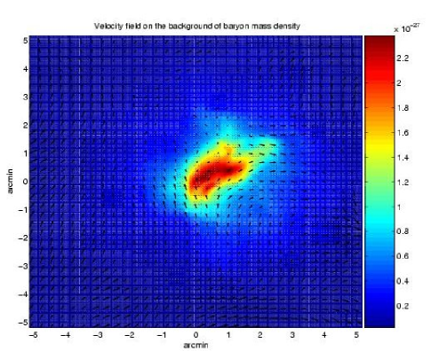
Figure 7: The velocity field is shown on the background of the baryon mass density; arrow length is linearly proportional to velocity magnitude). Color density scale is in units of $g/cm^{3}$.

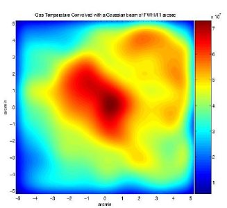
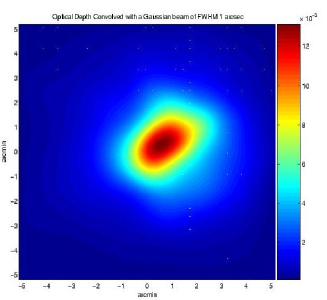
Figure 8: The cluster temperature (color scale in K) and optical depth maps are shown in the left and right figures, respectively.

Polarization maps on the sky plane are shown in Figures 9 & 10, with polarization levels specified in terms of the equivalent temperature. Unlike the case of spherical (Sazonov & Sunyaev 1999) or quasi-spherical (Lavaux et al. 2004) clusters, we obtain a more intricate polarization patterns and the quadrupole structure, which is absent in the spherically symmetric case, is evident. This pattern reflects the non-uniform gas distribution and an appreciable degree of non-sphericity of the cluster, which substantially affect primarily the double scattering polarization signals, essentially due to the fact that the second scattering is more likely to occur far from the cluster center (see also Sazonov & Sunyaev 1999, Lavaux et al. 2004). The level of polarization at the 545 GHz Planck frequency band, with a 4.5’ FWHM beam, can reach $\sim 80$ nK, but when convolved with a narrow beam 1’ FWHM profile, its peak value can be as high as $\sim 0.7\mu K$. This level definitely grazes the threshold of next generation experiments. It should be noted that we have considered a rich cluster with maximal optical depth of $\tau_{0}\approx 0.01$, but since this component is proportional to $\sim\tau^{2}$, typical values could be a factor $\sim 4$ lower or higher than the specific values quoted here. Also, this component was calculated at 545 GHz; lower levels of polarization are expected at lower frequencies.

Equations (28)-(30) for the double scattering kinematic component ($\propto\tau^{2}\beta$) can be written in the same form as equation (33), but with

$$h_{+,\times}=f_{+,\times}\star g\equiv\sum_{i=1}^{3}f_{i_{+,\times}}\star g_{i}$$ (35)

where

$$f_{i+}=\frac{X_{i}(X^{2}-Y^{2})}{r^{5}},\,\,\,f_{i\times}=\frac{2X_{i}XY}{r^{5}},\,\,\,g_{i}=n({\bf r})\beta_{i}({\bf r})$$ (36)

with $X_{i}$ ($i=1,2,3$) the components of the vector $(X,Y,Z)$. The results for the $\tau^{2}\beta$ component (for the central region of the simulation) are summarized in Figure 10. The level of polarization in absolute temperature units is $\sim 1-2$ orders of magnitudes smaller than the $\propto\tau^{2}\Theta$ component. Convolving with the Planck HFI and a Gaussian beam profile with FWHM of 1’, the peak values are $3$ nK and $25$nK, respectively, comparable to the level of the cosmological quadrupole polarization (section 3.1). As previously noted, both these components are frequency-independent, a fact that has obvious implications on the feasibility of separating these components out when the measurements will eventually reach the requisite sensitivity.

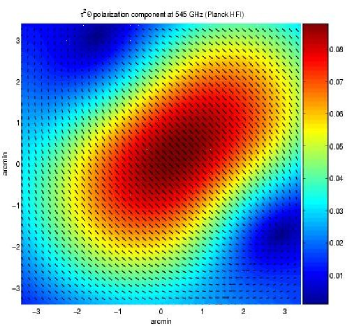
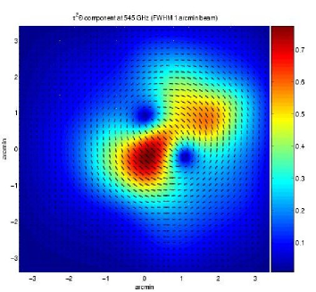
Figure 9: The $\tau^{2}\Theta$ polarization component convolved with the Planck HFI 4.5’ FWHM beam (left) and with a FWHM 1’ beam (right). Color scale is in $\mu$K.

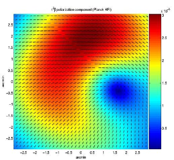
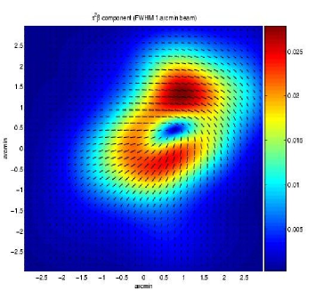
Figure 10: The $\tau^{2}\beta$ polarization component convolved with the Planck HFI 4.5’ FWHM beam (left) and with a FWHM 1’ beam (right). Color scale is in $\mu$K.

We end with a summary of the main result of this section: Most polarization signals induced by scattering of the CMB in clusters are substantially smaller than $1\,\mu$K. An exception is the polarization induced by the double scattering thermal effect. Convolving the predictions for this component in the simulated cluster with a FWHM 1’ beam, we find that the effective polarization signal is about $\sim 1\,\mu K$. The much improved CMB observational capabilities - with projected sensitivities around $1$ $\mu$K and arcminute angular resolution - will make it feasible to measure the dominant polarization signals in clusters by upcoming experiments, thereby supplementing X-ray and (total intensity) S-Z measurements to probe IC gas properties and cluster morphology.

Acknowledgment: Work at Tel Aviv University was supported by Israel Science Foundation grant 225/03.

References

- [1] Bardeen J.M., Bond J.R., Kaiser N., Szalay A.S. 1986, ApJ, 304,15
- [2] Bowden, M., et al. 2004, MNRAS, 349, 321
- [3] Bryan, G.L., Norman, M.L., Stone, J.M., Cen, R., & Ostriker, J.P. 1995, Compute. Phys. Commun, 89, 149
- [4] Carlstrom,J.E., Holder, G.P., & Reese, E.D. 2002, ARA& A, 40, 643
- [5] Carroll S.M., Press W.H., Turner E.L. 1992, ARAA, 30, 499
- [6] Chandrasekhar, S. 1950, ‘Radiative Transfer’, Oxford, Clarendon Press
- [7] Colafrancesco S., Mazzotta P., Rephaeli Y., & Vittorio N. 1994, ApJ, 433, 454
- [8] Colafrancesco S., Mazzotta P., Rephaeli Y., & Vittorio N., 1997 ,ApJ, 479, 1
- [9] De Petris, M., et al. 2002, ApJ, 574, L119
- [10] Eisenstein, D.J. & Hut, P. 1998 ApJ, 498, 137
- [11] Itoh, N., & Nozawa, S. 2004, A&A, 417, 827
- [12] Komatsu E., & Seljak U. 2002, MNRAS, 336, 1256
- [13] Koyama K., Soda J., Taruya A. 1999, MNRAS, 310, 1111
- [14] Kuo C.L. et al. 2004, ApJ, 600, 32
- [15] Kurk J., Venemans B., Röttgering H., Miley G., Pentericci L. 2004, in Plionis M., ed., Multiwavelength Cosmology. Kluwer, Dordrecht, preprint (astro-ph/0309675)
- [16] Lavaux, G., Diego, J.M., Mathis, H., & Silk, J. 2004, MNRAS, 347, 729
- [17] Mason B., Pearson T.J., Readhead A.C.S., Sheperd M.C., Sievers J.L., Udomprasert P.S., Cartwright J.K., Farmer A.J., et al. 2003, ApJ, 591, 540
- [18] Mathis H., Diego J.M., Silk, J. 2004, MNRAS, 353, 681
- [19] McEwen, J.D., et al. 2006, astro-ph/0604305
- [20] Miley G.K. et al. 2004, MNRAS, 427, 47
- [21] Molnar S.M., & Birkinshaw M. 2000, ApJ, 537, 542
- [22] Mullis C.R. et al. 2003, ApJ, 594, 154
- [23] O’Shea, B.W., et al. 2004, ‘Adaptive Mesh Refinement - Theory and Applications’, Eds. T. Plewa, T. Linde & V. G. Weirs, Springer Lecture Notes in Computational Science and Engineering, 341
- [24] Peebles P.J.E. 1999, ApJ, 510, 523
- [25] Press W.H., & Schechter P. 1974, ApJ, 187, 425
- [26] Rephaeli Y. 1995, ApJ, 445, 33
- [27] Rephaeli Y. 2005, Il Nuovo Saggiatore, 21, 38
- [28] Sadeh,S., & Rephaeli, Y. 2004, New Astronomy, 9, 159
- [29] Sadeh,S., Rephaeli, Y., & Silk, J. 2006, MNRAS, 368, 1583
- [30] Sazonov, S.Y., & Sunyaev, R. A. 1999, MNRAS, 310, 765
- [31] Shimon, M., & Rephaeli, Y. 2004, New Astronomy, 9, 69
- [32] Shimon M., Rephaeli Y., O’Shea B.W., & Norman M. L. 2006, MNRAS, 368, 511
- [33] Springel V., White M., & Hernquist L. 2001, ApJ, 549, 681
- [34] Sunyaev, R.A., & Zeldovich, Y.B. 1980, MNRAS, 190, 413
- [35] Vikhlinin A., McNamara B.R., Forman W., Jones C., Quintana J., Hornstrup A. 1998, ApJ, 498, L21