VERA 22 GHz fringe search survey

Abstract

This paper presents results of a survey search for bright compact radio sources at 22 GHz with the VERA radio-interferometer. Each source from a list of 2494 objects was observed in one scan for 2 minutes. The purpose of this survey was to find compact extragalactic sources bright enough at 22 GHz to be useful as phase calibrators. Observed sources were either a) within 6 degrees of the Galactic plane, or b) within 11 degrees from the Galactic center; or c) within 2 degrees from known water masers. Among the observed sources, 549 were detected, including 180 extragalactic objects which were not previously observed with the very long baseline interferometry technique. Estimates of the correlated flux densities of the detected sources are presented.

1. Introduction

VLBI Exploration of Radio Astrometry (hereafter VERA) is a Japanese VLBI array dedicated to phase-referencing astrometry to explore the Milky Way Galaxy (Honma et al. 2000a; Kobayashi et al. 2004). VERA observes Galactic H₂O and SiO maser sources and determines their parallax and proper motions at the 10 microarcsec accuracy level. Based on the high-precision astrometry of $\sim$1000 maser sources, VERA will study the three-dimensional structure and dynamics of the Galaxy’s disk and bulge, revealing the true shape of the bulge and spiral arms, its precise rotation curve and the distribution of dark matter.

The VERA array consists of four 20-m diameter radio telescopes spread over Japan, covering baselines ranging from 1000 km to 2300 km. Unlike other VLBI stations, VERA telescopes are equipped with a dual-beam system (Kawaguchi et al. 2000), with which one can simultaneously observe two sources separated from each other by up to a hundred times the telescope’s primary beam size. With such a system, VERA can observe a Galactic maser source and an extra-galactic calibrator source at the same time and perform relative astrometry of the Galactic maser source with respect to the extra-galactic calibrator, which serves as a position reference. Simultaneous observations of two sources, rather than switching observations with single-beam telescopes, are expected to be more effective in canceling out the tropospheric fluctuations, which are the main source of position error in differential VLBI astrometry at 22 GHz or higher frequency. In fact, preliminary results from VERA’s dual-beam system observations have already shown its high capability of phase-referencing to reach down to 10 microarcsecond level accuracy (Honma et al. 2003), and now monitoring of several bright maser sources is on-going to produce initial results from the VERA.

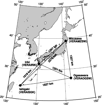
Figure 1.— VERA network.

In order to observe a pair of two adjacent sources with VERA, the separation angle of the pair must be less than $2.\!{}^{\circ}2$. This is not only a mechanical limit of VERA’s dual-beam system, but also a practical limit for effective phase referencing to achieve 10 microarcsec accuracy, i.e., the reference source needs to be close enough to the target maser to remove the tropospheric fluctuations sufficiently. Therefore, the existence of calibrators close to target sources is crucial to successful VERA observations. If we assume a uniform density of calibrators in the sky plane, $\sim$ 2700 calibrators are required in the whole sky to find a calibrator within $2.\!{}^{\circ}2$ of any sky position (a circle with radius of $2.\!{}^{\circ}2$ covers 0.0046 steradians in the sky; thus $4\pi/0.0046\approx 2700$ are necessary). Practically though, more sources are needed because the distributions over the sky is not uniform.

To date, there have been many efforts to find good calibrators observable with VLBI. The pioneering work of Cohen & Shaffer (1971) provided the first catalogue of source positions determined with VLBI, which contained 35 strong sources. In 1998 the International Celestial Reference Frame (ICRF) catalogue of 667 sources produced by analyzing VLBI observations made in the framework of space geodesy programs was published by Ma et al. (1998). At present, the most massive survey of compact calibrators is the VLBA Calibrator Survey, hereafter VCS, performed in 1994–2005 (Beasley et al. 2002; Fomalont et al. 2003; Petrov et al. 2005, 2006), and Kovalev et al. (submitted to AJ, 2006). After the fifth VCS campaign, the NASA catalogue 2005f_astro of all sources detected in the absolute astrometry mode at 2.2 GHz and/or 8.6 GHz frequency bands (S and X) contains 3481 sources. Among them, 85% are acceptable as calibrators for the VLBA. Nevertheless, in the sky area at $\delta\geq-40^{\circ}$, which is observable with the VERA, the probability of finding an X/S calibrator with correlated flux density over 60 mJy within $2.\!{}^{\circ}2$ of any position is $\sim$70% (Petrov et al. 2006), indicating that more calibrators are needed in order to observe all maser sources with VERA. Moreover, maser sources tend to be confined to the Galactic plane, because they are basically located in the Galaxy’s disk, but the density of known calibrators near the Galactic plane is even lower than that in other sky regions. This is due to the strategies used to find compact calibrators: the list of candidates was based on low resolution sky surveys that severely suffered from strong radio foreground in the Galactic plane. Besides, some past surveys, JVAS (Wrobel et al. 1998), VCS1, VCS3, VCS4, specifically avoided the Galactic plane. To overcome this problem, a calibrator survey in the Galactic plane has been done by Honma et al. (2000b) finding more than 50 new calibrators at $|b|\leq 5^{\circ}$, but still many more calibrators in this region are needed.

For these reasons, we have been performing the Galactic Plane Survey of compact radio sources, hereafter GaPS, based on the VERA and VLBA observations. The objective of this campaign is to provide a list of calibrators for dual-beam VERA observations of H₂O masers at 22 GHz. Our strategy for GaPS is two-fold: first, we observe a wide list of candidate sources with the VERA, and then observe a narrow list of detected sources with the VLBA in order to determine their positions at the 1–10 nrad level of accuracy and to obtain high quality maps. In this paper, we present results from the first part of the GaPS project, the fringe search observations with the VERA, reporting the detection of 180 new compact sources. In section §2 we describe our approach to the selection of candidates, scheduling and observations. In section §3 we describe analysis of the observations. Results are discussed in section §4 and concluding remarks are given in section §5.

2. Observations

2.1. Source selection

We searched for compact extragalactic sources with correlated flux density $>100$ mJy at spacings $\sim\!10^{8}$ wavelengths at 22 GHz in the following zones: a) $|b|<6^{\circ}$ and $\delta>-40^{\circ}$; b) within an $11^{\circ}$ radius of the Galactic center; and c) within $2.\!^{\circ}2$ of objects listed in the 2nd update of Arcetri Catalog of H₂O maser sources (Valdettaro et al. 2001) and the stellar masers catalogue of Benson et al. (1990).

First, we combed through the wide list of 3481 known compact sources observed under absolute astrometry programs at S/X bands. Among them, 510 fall in our zones of interest. Also among the 3481 known compact sources, 252 objects have been observed under the K/Q band survey in 2002–2005 (Fey et al. 2005; Jacobs et al. 2005), and can be considered as confirmed K-band calibrators. But only 16 of these fall in our zones of interest. The first list of targets was formed from the 510 known X-band calibrators, except 16 objects observed with the K/Q band survey. The purpose of including known X/S calibrators in the list of candidate sources was to check whether they are bright enough at K band to be detected. It was expected that not all of these will be detected with the VERA, since although they have correlated flux densities above 60 mJy at X-band, their correlated flux densities at K-band may be below the VERA detection limit, and, therefore, not suitable as calibrators for VERA.

Second, we searched the CATS database (Verkhodanov et al. 1997) containing almost all radio catalogs to find flux density measurements at radio frequencies 1.4 MHz and higher. We selected the sources with at least two measurements of the flux density and found their spectral index by fitting a straight line to the log(F)/log(f) dependence, where $F$ is the flux density and $f$ is the frequency. The flux density was extrapolated to 22 GHz. Those sources in the zone of our interest, which had extrapolated flux density $>100$ mJy at 22 GHz, and which were not observed in the absolute astrometry mode, were put in the second list of targets, in total 1901 new sources.

2.2. Scheduling

The list of target sources was split into two group: the first group, of 1386 objects, within $6^{\circ}$ of the Galactic plane or within $11^{\circ}$ from the Galactic center; and a second group, of 1032 sources, within $2.\!{}^{\circ}2$ from known galactic maser sources. The first group had priority in scheduling. Among target sources, 94% were observed in one scan of 120 s, and 6% were observed in two scans. Observing schedules were prepared using the following procedure. A source in the target list, which was not observed in previous experiments and which had the highest elevation at the station of VERZMZSW, was selected as the first objects in the schedule. In order to select the next source, the pool of target sources was examined, and for each source, which was at least $10^{\circ}$ above the horizon and which was not previously observed, a score was computed: $S=100/T_{slew}+30*(20-\delta)+0.2*E_{min}$ where $T_{slew}$ is the slewing time in seconds, $\delta$ is the source declination, in degrees, and $E_{min}$ is the minimum elevation of the source among the network stations, in degrees. The source from the first group with the maximum score was put in the schedule. If no source from the first group was visible, the source with the highest score from the second group was put in the schedule. Then the procedure was repeated. The slewing rate of VERA stations is $2^{\circ}\,s^{-1}$ and acceleration is $2^{\circ}\,s^{-2}$. The antenna control hardware requires adding a margin of 10 seconds to slewing time, and the slewing time should be rounded to the next 4 s. Measurement of system temperature takes an additional 30 seconds. System temperature was measured either every 5 scans or when the antennas moved more than $10^{\circ}$ from the previous measurement, whichever occurs first. In addition to targets, observations of amplitude calibrator sources were scheduled every hour. At the beginning and at the end of each session a very strong source, a fringe finder, was observed. The amplitude calibrator sources were taken from the list of 252 sources observed with the K/Q band survey. The average density of observations was 22 scans per hour.

2.3. Observations

GaPS survey observations were scheduled mainly within gaps between regular VERA observations (table 1). Some observations were performed only at three antennas while one of the stations was not available.

Table 1Observing sessions

(1)	(2)	(3)	(4)	(5)
r05284b	2005 Oct. 11  08:20	7.0	3	1.0
r05285b	2005 Oct. 12  08:20	7.0	4	1.0
r05332b,c	2005 Nov. 28  12:20	10.8	4	1.0
r05335b	2005 Dec. 01  11:00	12.5	4	1.0
r05343b	2005 Dec. 09  15:00	8.5	4	0.1
r05348a	2005 Dec. 14  09:00	14.0	3	1.0
r05349a	2005 Dec. 15  10:00	20.0	3	1.0
r05350a	2005 Dec. 16  07:00	7.5	3	1.0
r05350b	2005 Dec. 16  14:55	8.5	3	1.0
r05353d	2005 Dec. 19  04:00	5.5	3	1.0
r05359d	2005 Dec. 25  02:00	7.0	4	0.1
r06052b	2006 Feb. 21  18:00	13.0	4	0.1
r06054a	2006 Feb. 23  19:00	11.0	4	0.1
r06059b	2006 Feb. 28  18:00	16.0	4	0.1

Note. — (1) session name; (2) start date; (3) duration in hours; (4) # stations; (5) Accumulation period length in seconds.

The left circular polarization in band 21.97–22.47 GHz band was received, sampled with 2 bit quantization, and filtered using the VERA digital filter (Iguchi et al. 2005) before being recorded onto magnetic tapes. The digital filter split the data within the 500 MHz band into 16 frequency channels of 16 MHz width each, equally spaced with spacing 32 MHz. The data were recorded with the SONY DIR2000 recorder at 1 Gbps rate.

3. Data analysis

Correlation was carried out on the Mitaka FX correlator (Chikada et al. 1991) with a spectral resolution of 250 kHz. Thus, the amplitude and phase of the cross correlation function at 64 spectral channels within each of the 16 frequency channels was determined. The correlator writes the output in the native CODA format. The output was re-formated to the FITS-IDI format (C. Flatter, (1998) unpublished). One part of the observing sessions was correlated with accumulation periods of 0.998 s, and another part was correlated with accumulation periods of 0.1 s.

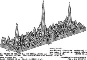
Figure 2.— Fringe amplitude versus delay and delay rate for a strong source.

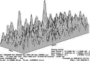
Figure 3.— Fringe amplitude versus delay and delay rate for a marginally detected source.

The data were analyzed with program PIMA. The first step of analysis was fringe fitting. The group delay and delay rate that maximize the fringe amplitude were sought for each baseline independently. The spectrum of the cross-correlation function was presented as a two-dimensional array, with the first dimension running over frequency channels, and the second dimension running over accumulation periods. The size of the matrix was $960\!\times\!120$ for scans with accumulation periods of 1 s and $1920\!\times\!1200$ for data with accumulation periods of 0.1 s. The grid was extended to $4096\!\times\!512$ and $8192\!\times\!4096$ for the data with 1 s and 0.1 s accumulation periods, respectively, with an oversampling factor of four by padding extended elements with zeros. The amplitudes of the cross-correlation function was normalized by dividing it by the square root of the product of the autocorrelation of the recorded data at each station of the baseline. The two-dimensional fast Fourier transform was performed. The first dimension of the Fourier transform runs over group delays from 0 through 4 mks with steps of 0.49 ns, and the second dimension runs over delay rates from 0 through $4.6\cdot 10^{-11}$ with steps of $0.9\cdot 10^{-13}$ for the data with 1 s accumulation periods, and from 0 through $4.6\cdot 10^{-10}$ with the step of $1.1\cdot 10^{-13}$ for the data with the accumulation periods of 0.1 s. The coarse search for the maximum of the correlation amplitude was performed over results of the Fourier transform. In the worst case, when the maximum of the correlation amplitude falls just between the nodes of the grid, the amplitude is reduced by $\mbox{sinc}^{2}(\pi/(2v))$, where $v$ is the oversampling factor. When $v=4$, in the worst case the amplitude is reduced by $\frac{16(2-\sqrt{2})}{\pi^{2}}=0.95$. The oversampling is important for detecting weak sources. The fine search of the correlation maximum is performed by the consecutive direct Fourier transform at a grid $3\!\times\!3$ around the maximum with reducing spacings of the grid by half at each step of an iteration. Three iterations of the fine search were performed. Examples of fringe amplitude plots versus trial delay and delay rate for a weak and a strong source are shown in figures 2 and 3.

Observations of strong sources with signal to noise ratios exceeding 120 were used for evaluation of a baseline dependent bandpass calibration. The phase of the bandpass calibration was determined as a residual phase with the opposite sign at each spectral channel after subtracting the multi-band fringe phase. A linear model was fitted into individual phases at spectral channels within each frequency channel. The amplitude of the band-pass was determined as the ratio of the fringe amplitude at an individual spectral channel to the maximum amplitude within the band. The estimate of the maximum amplitude across the band was found as the maximum value of the amplitude across 1024 spectral channels minus the doubled standard deviation of the amplitude at an individual spectral channel. It was found that the bandpass is stable between experiments, so the bandpasses over all experiments were stacked and averaged. An example of the bandpass calibration is shown in figures 4 and 5. The complex bandpass calibration was applied to all observations, i.e. the $uv$ data were multiplied with the complex bandpass before the fringe search. This technique increased the fringe amplitude by 5–15%.

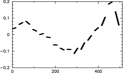
Frequency MHz

Figure 4.— The phase of the bandpass calibration at baseline veramzsw/veraogsw.

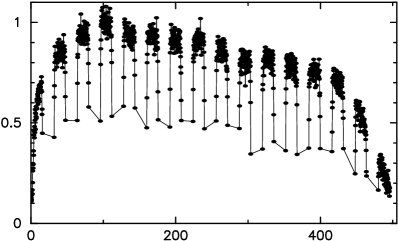
Frequency MHz

Figure 5.— The amplitude of the bandpass calibration at baseline veramzsw/veraogsw.

3.1. Calibration

System temperatures including atmospheric attenuation were measured with the chopper-wheel method (Ulich & Haas 1976). A microwave absorber at ambient temperature was inserted just in front of the feed horn at the beginning of each scan, and the received total power was measured with a power meter. Using the measured total power for the blank sky and the absorber, we can determine the temperature scale automatically corrected for the atmospheric attenuation. The system temperatures during the best weather conditions were 100–200 K. However, at typical weather conditions, $T^{\star}_{sys}$ were 200-500 K depending on the elevation of observed sources, reaching 2000 K at low elevations and during adverse weather conditions. Figures 6 and 7 illustrate recorded system temperatures at two stations at good and adverse weather conditions. The uncertainty in the temperature scale was estimated to be 10%, mainly due to the assumption that the ambient temperature is the same as the air temperature

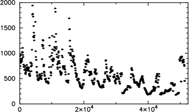
Time s

Figure 6.— System temperature corrected for the atmosphere opacity versus time from beginning of observing session at veraisgk on 2005.12.14.

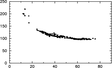
Elevation deg

Figure 7.— System temperature corrected for the atmosphere opacity versus elevation in degrees at veramzsw on 2005.12.09.

The aperture efficiency of each antenna was 45–52% in the 22 GHz band, which was measured by observing the continuum emission from Jupiter once per year. The accuracy of the aperture efficiency measurement was typically 2-5%. The antenna gain does not show elevation dependency in the elevation range 10–$90^{\circ}$.

Amplitude calibration was performed in two steps. First, the amplitude conversion factor was computed for each observation based on measurements of system temperature and antenna efficiency as $A=\sqrt{\frac{T^{\star}_{1sys}\,T^{\star}_{2sys}}{g_{1}\,g_{2}}}$ where $g_{i}$ is the antenna gain. This factor converts dimensionless fringe amplitude to correlated flux density. Then the multiplicative correction to the conversion factor was computed for each observation of the amplitude calibrator at each baseline as $\delta A=\frac{F_{kq}}{F_{obs}}$ where $F_{kq}$ is the correlated flux density from maps from the KQ survey and $F_{obs}$ is the observed correlated flux density. The correction $\delta A$ was averaged over all amplitude calibrators within an individual observing session. The scatter of the individual estimates of the correction provided the measure of errors of amplitude calibration: 20–25%. Since for the vast majority of sources, only 3 or 6 values of fringe amplitude and phase were determined, no attempt to make maps was made.

3.2. Detection limit

Strong sources have a noticeable peak in plots of fringe amplitude versus trial delay and delay rate, for instance figure 2. The presence of noise will force the fringe search process to find a peak in such a plot even in the absence of a signal from the source. For each observation we need to evaluate the probability of false detection. In the absence of signal the amplitude of the cross correlation function $z$ has Rayleigh distribution (Papolius 1965):

$$p(z)=\frac{\displaystyle z}{\displaystyle\sigma^{2}}e^{-(\frac{z^{2}}{2\sigma^{2}})}$$ (1)

where $\sigma$ is the standard deviation of the real and imaginary part of the cross correlation function. The noise level of fringe amplitudes was evaluated for each observation. At the grid of cross correlation function spectrum 16384 points were randomly taken and the average amplitude was computed. In order to insure that no data points with signal were taken, an iterative procedure removed all the points which exceeded the average by more than 4 times. The average amplitude of noise in the spectrum was considered as an estimate of the mathematical expectation of the noise, ${\cal E}(z)=\sqrt{\pi/2}\,\sigma$. In the case when all points of the spectrum are statistically independent, the cumulative probability for the maximum of $n$ points is (Thompson et al. 2001)

$$P(z)=\left(1-e^{-(\frac{z^{2}}{2\sigma^{2}})}\right)^{n}$$ (2)

Then, differentiating this expression, we find the probability distribution density of the ratio of the maximal fringe amplitude to the averaged noise at points in the spectrum with no signal, $s=z_{max}/<\!\!z\!\!>$:

$$p(s)=\frac{\displaystyle 2}{\displaystyle\pi}\frac{\displaystyle n}{\displaystyle<\!\!z\!\!>}\,s\,e^{-\frac{s^{2}}{\pi}}\left(1-e^{-\frac{s^{2}}{\pi}}\right)^{n-1}$$ (3)

It should be emphasized that expression 3 is valid if all points of the spectrum are independent. This a priori distribution density is an approximation, which is valid only partially due to oversampling and deviation of the bandpass from a rectangular shape. Using the sample of achieved signal to noise ratios, we computed the a posteriori distribution density. We assumed that the a posteriori distribution can be approximated as a function like expression 3 with effective parameters $<\!\!z\!\!>_{\mbox{eff}}$ and $n_{\mbox{eff}}$. We found parameters of the distribution which minimize residuals between the a priori and a posteriori distribution densities in the range of signal to noise ratios [3,  6.5] by searching through the space of trial values using the brute force algorithm. Plots of the a posteriori maximum of the signal to noise ratios and its approximation for the case of accumulation periods lengths of 1 s and 0.1 s are presented in figures 8 and 9.

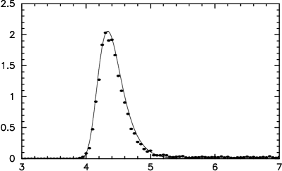
s

Figure 8.— The distribution density of the achieved signal to noise ratios (points) and the regression curve (continuous line) $p(s)=\frac{\displaystyle 2}{\displaystyle\pi}\frac{\displaystyle n_{\mbox{eff}}}{\displaystyle<\!\!z_{\mbox{eff}}\!\!>}\,s\,e^{-\frac{s^{2}}{\pi}}\left(1-e^{-\frac{s^{2}}{\pi}}\right)^{n_{\tiny\mbox{eff}}-1}$ for scans with accumulation periods 1.0 s. $<\!\!z_{\mbox{eff}}\!\!>=1.101,n_{\mbox{eff}}=183000$.

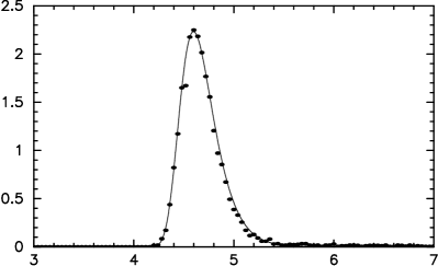
s

Figure 9.— The distribution density of the achieved signal to noise ratios (points) and the regression curve (continuous line) $p(s)=\frac{\displaystyle 2}{\displaystyle\pi}\frac{\displaystyle n_{\mbox{eff}}}{\displaystyle<\!\!z_{\mbox{eff}}\!\!>}\,s\,e^{-\frac{s^{2}}{\pi}}\left(1-e^{-\frac{s^{2}}{\pi}}\right)^{n_{\tiny\mbox{eff}}-1}$ for scans with accumulation periods 0.1 s. $<\!\!z_{\mbox{eff}}\!\!>=1.091,n_{\mbox{eff}}=989000$.

Using effective parameters of the a priori distribution, we can compute the probability that a given observation with the signal to noise ratio $s$ belongs to the population of observations without signal from a source as

$$N(s)=1-\displaystyle\int\limits_{0}^{s}p(s)\,ds=1-\frac{1}{<\!\!z_{\mbox{eff}}\!\!>}\left(1-e^{-\frac{s^{2}}{\pi}}\right)^{n_{\tiny\mbox{eff}}}$$ (4)

Examining plots of the a posteriori distribution density, we conclude that at the range of signal to noise ratios [3.5, 6.5] the share of points which belongs to detected sources is insignificant. Neglecting the population of observations with detected sources slightly inflated our estimates of the probability that an observation belongs to the population of data without signal and makes our estimates of the probability of detection a bit more conservative.

Each source was observed $m$ times, $m$ typically being in the range 3–6. At a given series of signal to noise ratios, a source has $k$ observations with signal to noise ratio greater than $s_{lim}$. The probability of false detection $p_{lim}$ corresponds to it. Then for the case when $p_{lim}$ is small that we can neglect terms of $p_{lim}^{2}$, the probability that this may happen due only to the noise in the data, i.e. a source was not detected in neither of $k$ observations, is

$$N_{k}=C^{k}_{m}\displaystyle\prod_{i=1}^{i=k}N(s_{i})$$ (5)

We used this expression in order to compute the probability of false detection for each source. The value $p_{lim}=0.05$ was used for computations.

4. Results and discussion

We split the list of 2494 sources into three groups: not detected if the probability of false detection is higher than $10^{-2}$; marginally detected if the probability of false detection is in the range of $[10^{-5},\,10^{-2}]$; and reliably detected if this probability is less than $10^{-5}$.

Careful analysis revealed that 16 detected sources are known water masers. The H₂O line was within the recorded bandwidth. We made a trial fringe search using only one frequency channel which included the water maser line. The fringe amplitude decreased by factor of 4 for continuum sources and increased by the same factor for maser sources.

The catalogue of 533 detected sources, which are not masers, is listed in table 2. Source coordinates are taken from the NVSS catalogue (Condon et al. 1998). Column /5/ shows the detection status: D — reliably detected, M — marginally detected. The correlated flux density in jansky is at three ranges of baseline projections are given in columns /6/, /7/, /8/: in the range of [0, 70] megawavelengths; in the range of [70, 100] megawavelengths; and in the range of [100, 200] megawavelengths. Column /9/ gives the probability of false detection, if it exceeds $10^{-5}$, or zero, if it is less than $10^{-5}$. Column /10/ gives a flag denoting whether the source was previously detected in the X/S surveys (KNO) or not (NEW).

Table 2List of detected continuum spectrum sources

J2000 name	B1950 name	$\alpha$ (J2000)	$\delta$ (J2000)	(5)	(6)	(7)	(8)	(9)	(10)
J0001+6051	2358+605	00:01:07.09	+60:51:22.8	D	$\cdots$	0.16	0.21	0.0	KNO
J0005+5428	0002+541	00:05:04.36	+54:28:24.9	D	$\cdots$	0.32	0.28	0.0	KNO
J0006+5050	0003+505	00:06:08.29	+50:50:03.4	D	$\cdots$	$\cdots$	0.17	0.0	NEW
J0014+6117	0012+610	00:14:48.79	+61:17:43.5	D	0.29	0.25	0.33	0.0	KNO
J0019+2021	0017+200	00:19:37.85	+20:21:45.6	D	$\cdots$	0.89	0.91	0.0	KNO
J0019+7327	0016+731	00:19:45.78	+73:27:30.0	D	1.24	1.35	1.28	0.0	KNO
J0021-1910	0018-194	00:21:09.37	-19:10:21.3	M	0.53	0.09	$\cdots$	5.D-03	NEW
J0027+5958	0024+597	00:27:03.28	+59:58:52.9	D	0.35	0.49	0.28	0.0	KNO
J0037-2145	0034-220	00:37:14.79	-21:45:24.5	D	$\cdots$	0.33	0.12	5.D-06	NEW

Note. — Table 2 is presented in its entirety in the electronic edition of the Astronomical Journal. A portion is shown here for guidance regarding its form and contents. Units of right ascension are hours, minutes and seconds; units of declination are degrees, minutes and seconds; units of flux density is jansky.

Table 3 lists 1945 non-detected sources. Columns /5/, /6/ and /7/ provide the minimum, average and maximal upper limit of the correlated flux density. These quantities are computed on the basis of the calibrated gain of the interferometer considering what correlated flux density would provide a signal to noise ratio of 6.0. Column /8/ gives the number of observations used in the analysis, and column /9/ gives a flag denoting whether the source was previously detected at the X/S survey (KNO) or not (NEW).

Table 3List of not detected sources

J2000 name	B1950 name	$\alpha$ (J2000)	$\delta$ (J2000)	(5)	(6)	(7)	(8)	(9)
J0000+3252	2358+326	00:00:49.72	+32:52:56.5	0.11	0.15	0.18	3	NEW
J0000+5539	2357+553	00:00:20.45	+55:39:08.6	0.13	0.15	0.16	3	NEW
J0001+6443	2358+644	00:01:14.95	+64:43:01.1	0.20	0.33	0.88	9	NEW
J0002+5510	2359+548	00:02:00.47	+55:10:38.0	0.15	0.15	0.16	2	NEW

Note. — Table 3 is presented in its entirety in the electronic edition of the Astronomical Journal. A portion is shown here for guidance regarding its form and contents. Units of right ascension are hours, minutes and seconds; units of declination are degrees, minutes and seconds; unit of flux density is jansky.

Table 4Statistics of observed sources

Category	Detected	Not detected
New, continuum spectrum	180	1721
Known, water masers	16	$\cdots$
Known X/S, continuum spectrum	353	224
Known X/S/K, amplitude calibrators	73	3
Total	549	1945

The statistics of the sample of observed sources is given in table 4. VERA detected $~{}60$% of the known X/S sources and $~{}10$% of the new sources. These results are somewhat disappointing. With the best weather conditions VERA is able to detect sources as weak as 100 mJy with 2 minute integration times. However, even in winter, adverse weather conditions significantly deteriorated the detection limit. We show in figure 10 the cumulative probability function that a source will have a fringe amplitude signal to ratio limit greater than 6.0 among 14 observing sessions. This detection limit was computed on the basis of the calibrated gain. This probability distribution characterizes the current averaged VERA single beam sensitivity in winter when observations are carried out with the integration times of 120 s.

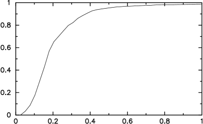
Flux density (Jy)

Figure 10.— Cumulative probability function for a source to have signal to noise ratio above the detection limit 6.0 over 14 observing sessions with VERA at 22 GHz.

a

Since the 2005f_astro X/S catalogue contains 3297 objects within the declination zone $>-40^{\circ}$, the zone which the VERA can observe, and approximately 60% of the sources from this catalogue were detected, we can roughly estimate that the VERA can detect $~{}2000$ sources from that list. To date, 252 sources were detected at K-band with the VLBA in the K/Q survey, 280 other known X/S calibrators and 180 new sources were detected with the VERA in this campaign, and 64 sources were detected with VERA at various other experiments. In total, the pool of confirmed K band calibrators is 776 objects.

5. Concluding remarks

In the 2005/2006 winter campaign $\sim 2500$ sources were observed with the VERA during 148 hours. The target sources were either within $6^{\circ}$ of the Galactic plane, or within $11^{\circ}$ of the Galactic center, or within $2.\!{}^{\circ}2$ of SiO or H₂O masers. Among them, 533 continuum spectrum and 16 maser sources were detected, including 180 continuum spectrum sources not previously observed with VLBI. The estimates of the correlated flux densities in the ranges [0, 70], [70, 100], and [100, 200] megawavelengths were evaluated. For 1945 non-detected sources the upper limits of their correlated flux densities were evaluated.

The distribution of detected sources over the sky is shown in figure 11. All detected sources are scheduled for observations with the VLBA at 22 GHz in June-October 2006 for imaging and determination of their positions with 1–10 nanoradian accuracies. Tables of detected and non-detected sources, plots of system temperatures, fringe plots, and other auxiliary information related to this campaign can be found on the Web at http://lacerta.gsfc.nasa.gov/vlbi/fss.

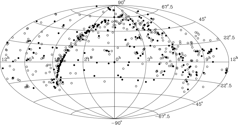
Figure 11.— The distribution of detected sources over the sky. Disks designate new compact source not observed before with VLBI, circles designate known sources observed before at X-band with the VLBA.

Analysis of the VERA fringe survey data shows that the probability of detecting a 100 mJy source with 120 s of integration time is about 10%; the probability of detecting a 200 mJy source is 60%; and the probability of detecting a 300 mJy source is 80%. Future development a next generation water vapor radiometer (Kawaguchi (2006), private communication) promises to allow increasing the integration time and, thus, to improve VERA sensitivity.

References

- Beasley et al. (2002) Beasley, A. J., Gordon, D., Peck, A. B., Petrov, L., MacMillan, D. S., Fomalont, E. B., & Ma, C. 2002, ApJS, 141, 13
- Benson et al. (1990) Benson P. J., Little-Marenin I. R., Attridge J., Blais K., Randolph D., Woods T., Rubiera M., Keefe H. 1990, ApJS, 74, 911
- Chikada et al. (1991) Chikada, Y., et al. 1991, in Frontiers of VLBI, ed. H. Hirabayashi, M. Inoue, & H. Kobayashi, Tokyo: Universal Academy Press, 79
- Cohen & Shaffer (1971) Cohen, M. H. & Shaffer, D. B. 1971, AJ, 76, 91.
- Condon et al. (1998) Condon, J. J., Cotton, W. D., Greisen, E. W., Yin, Q. F., Perley, R. A., Taylor, G. B., Broderick, J. J. 1998, AJ, 115, 1693
- Fey et al. (2005) Fey A., Boboltz D. A., Charlot P., Fomalont E. B., Lanyi G. E., Zhang L. D. 2005, ASP Conference Series, 340, 514.
- Fomalont et al. (2003) Fomalont, E., Petrov, L., McMillan, D. S., Gordon, D., Ma, C. 2003, AJ, 126, 2562
- Honma et al. (2000a) Honma. M., Kawaguchi, N., Sasao, T. 2000, in Proc. SPIE vol. 4015 Radio Telescope, ed. H. R. Buthcer, 624
- Honma et al. (2000b) Honma, M. et al. 2000, PASJ, 52, 631
- Honma et al. (2003) Honma, M., et al. 2003, PASJ, 55, L57
- Iguchi et al. (2005) Iguchi, S., Kurayama, T., Kawaguchi, N., and Kawakami, K. 2005, PASJ, 57, 259
- Jacobs et al. (2005) Jacobs C. S., Lanyi G. E., Naudet C. J., Sovers O. J., Zhang L. D. 2005, ASP Conference Series, 340, 523.
- Kawaguchi et al. (2000) Kawaguchi, N., Sasao, T., Manabe, S. 2000, in Proc. SPIE, vol. 4015 Radio Telescope, ed. H. R. Buthcer, 544
- Kobayashi et al. (2004) Kobayashi, H., et al., 2004, Proceedings of the 7th Symposium of the European VLBI Network on New Developments in VLBI Science and Technology. ed. by R. Bachiller et al., 275
- Ma et al. (1998) Ma, C., Arias, E. F., Eubanks, T. M., Fey, A. L., Gontier, A. M., Jacobs, C. S., Sovers, O. J., Archinal, B. A., Charlot, P. 1998, AJ, 116, 516
- Papolius (1965) Papolius, A., Probability, Random variables and Stochastic Processes, McGraw-Hill, New York, 1965
- Petrov et al. (2005) Petrov, L., Kovalev, Y.Y., Fomalont, E., Gordon, D. 2005, AJ, 129, 1163
- Petrov et al. (2006) Petrov, L., Kovalev, Y.Y., Fomalont, E., Gordon, D. 2006, AJ, 131, 1872
- Thompson et al. (2001) Thompson, A. R., Moran, J. M., Swenson, G.W., Interferometry and synthesis in Radio astronomy, Wiley Sons, Inc., 2001
- Verkhodanov et al. (1997) Verkhodanov, O. V., Trushkin, S. A., Andernach, H., & Chernenkov, V. N. 1997, in ASP Conf. Ser. 125, Astronomical Data Analysis Software and Systems VI, ed. by G. Hunt, & H. E. Payne (San Francisco: ASP), 322
- Ulich & Haas (1976) Ulich, B. L., & Haas, R. W. 1976, ApJS, 30, 247
- Valdettaro et al. (2001) Valdettaro R. et al. 2001, A&A, 368, 845
- Wrobel et al. (1998) Wrobel, J. M., Patnaik, A. R., Browne, I. W. A., & Wilkinson, P. N. 1998, A&AS, 193, 4004