Fluxon Modeling of Low-Beta Plasmas

Abstract

We have developed a new, quasi-Lagrangian approach for numerical modeling of magnetohydrodynamics in low to moderate $\beta$ plasmas such as the solar corona. We introduce the concept of a “fluxon”, a discretized field line. Fluxon models represent the magnetic field as a skeleton of such discrete field lines, and interpolate field values from the geometry of the skeleton where needed, reversing the usual direction of the field line transform. The fluxon skeleton forms the grid for a collection of 1-D Eulerian models of plasma along individual flux tubes. Fluxon models have no numerical resistivity, because they preserve topology explicitly. Our prototype code, FLUX, is currently able to find 3-D nonlinear force-free field solutions with a specified field topology, and work is ongoing to validate and extend the code to full magnetohydrodynamics. FLUX has significant scaling advantages over conventional models: for “magnetic carpet” models, with photospheric line-tied boundary conditions, FLUX simulations scale in complexity like a conventional 2-D grid although the full 3-D field is represented. The code is free software and is available online. In this current paper we introduce fluxons and our prototype code, and describe the course of future work with the code.
 

1 Introduction

MHD modeling is key to understanding solar eruptive events and their effect on the heliospheric enviroment. Solar flares are known to be driven by magnetic reconnection (e.g. Sturrock et al. 1984) and coronal mass ejections (CMES) are generally tied to magnetic instability of one kind or another (e.g. Sturrock 1989; Amari and Luciani 1999; Antiochos et al. 1999; Chen and Shibata 2000; Fan and Low 2003; Roussev et al. 2003). Understanding and predicting such events requires numeric modeling of the plasma in the solar corona as it evolves under the line-tied boundary conditions imposed by the solar photosphere. Current MHD modeling software is not able to reproduce the conditions of the solar corona under controlled conditions, because numerical effects in the simulation dominate over their counterparts in the real corona for many physical situations. This is evident in the difficulty of maintaining strong current sheets or other stressed flux systems, such as filaments, for long periods of time; and in the difficulty of reproducing the rapidly varying heating rate in coronal loops and bright points.

Conventional magnetohydrodynamic models typically use Eulerian (fixed) grids, introducing nonphysical dissipative effects such as viscosity and resistivity. These dissipative effects dominate the behavior of quiescent structures with current sheets and may even destabilize simulated CME-bearing systems Lin and van Ballegooijen (2002), making modeling of solar evolution difficult at best. Further, numerical diffusion of both momentum (’numerical viscosity’) and magnetic field (’numerical resistivity’) are dependent on grid speed, so that Eulerian grid size is typically chosen to oversample the physical structure. The extra resolution is used to minimize the unwanted diffusion and preserve the plasma system for as much simulated time as possible. Oversampling by a factor of 10 in each dimension yields a factor of $10^{4}$ slowdown in the overall simulation, requiring huge facilities to simulate even simple systems in 3-D. Adaptive-mesh refinement improves performance significantly (e.g. Welsch et al. 2004; Lynch et al. 2003) but still requires oversampling.

Lagrangian grids eliminate numerical resistivity but add additional problems. For example, as the grid distorts with the plasma motion, the fidelity of discrete differential operators degrades. Fully Lagrangian treatments of the corona shear rapidly because fluid motion is decoupled in the cross-field direction.

To maximize the advantages of both the Eulerian and Lagrangian approaches to MHD modeling, we have developed a prototype fluxon modeling code, FLUX (the “Field Line Universal relaXer”), that is a hybrid between the two. In the low-$\beta$ regime, all forces are negligible when compared to the Lorenz force components; FLUX is essentially a force-free field solver that can support an independent plasma density parameter at each location in the simulation. FLUX demonstrates the fluxon method, and work is ongoing to add plasma pressure and related physical phenomena to the simulation framework. In the following sections, we briefly describe the basis of the fluxon numerical approach (§2), describe our code and its performance (§3), and discuss the direction of future work both on code development and on applications (§4).

2 Fluxon theory and implementation

The basis of the fluxon approach to numerical modeling is the analogy between field lines and an associated vector field: a field line map completely describes the associated magnetic field, and vice versa. This analogy has normally been used to visualize the magnetic field: the field vector value is calculated everywhere on a grid of values, and then interpolated to “shoot” field lines through the grid for visualization. But the analogy works in the reverse direction too: every physical property of the magnetic field may be described in terms of the behavior of individual magnetic field lines. In highly conductive plasmas, the field line description takes on more utility and meaning than in resistive physical systems, because field line topology is preserved under ideal MHD.

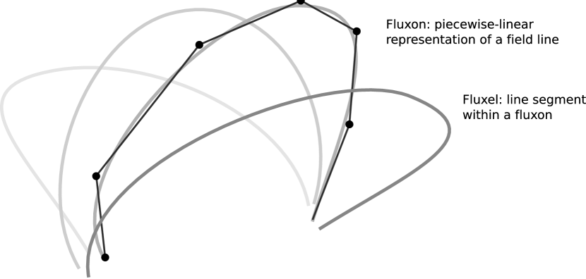
Figure 1: A fluxon representation of the magnetic field replaces smooth field lines (each of which represents an infinitesimal amount of flux) with piecewise-linear fluxons (each of which represents a small but finite amount of flux). Each fluxon is composed of flux elements, or fluxels, that represent small units of field-aligned length $ds$.

FLUX is currently a relaxation solver for force-free magnetic systems: the magnetic field is represented as a skeleton of piecewise linear curves, fluxons, each of which represents a finite quantum of magnetic flux contained in a thin volume around a central curve. Fluxons differ from conventional field lines in that a field line represents an infinitesimal amount of magnetic flux, while a fluxon represents a discrete, finite amount of magnetic flux; the word is also used, with approximately the same meaning, in the context of quantized magnetic systems such as Josephson junctions and quantum computers (e.g. Calidonna and Naddeo 2005; Ustinov et al. 1993). The magnetic field is considered to be nearly parallel to the fluxon everywhere in its neighborhood, so that each fluxon may be considered to represent a non-twisted flux tube and (as with conventional field lines) magnetic field strength may be calculated by determining the areal density of fluxons that pass through a plane perpendicular to the field direction. Other quantities such as field gradients may be calculated from the local geometry of the fluxons.

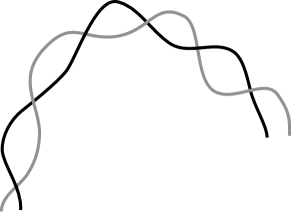
Figure 2: Two-fluxon system demonstrating representation of current. A computable current runs along the axis of the twisted loop.

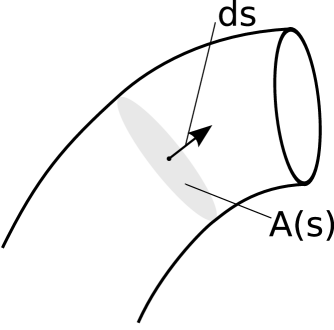
Figure 3: A curved flux tube carries flux $\Phi$ along its length; its geometry is parametrized by path length $s$ and its cross section is $A(s)$.

Each fluxon in a simulation arena is composed of an ordered collection of flux elements, or fluxels (Figure 1). A fluxel represents a small amount of field-aligned length $ds$, and the differential MHD equations are discretized using $d\Phi\Rightarrow\Phi_{0}$ (where $\Phi_{0}$ is the quantum of magnetic flux) and $ds\Rightarrow\Delta s$ (when calculating curvature and similar quanties). Each fluxel takes the same part in a fluxon simulation that a pixel (or voxel or grid element) takes in a conventional Eulerian simulation. In the current implementation, fluxels are line segments and their associated fluxons are thus piecewise-linear. One may imagine spline or other curvilinear interpolation, but the geometric calculations are greatly simplified by a piecewise linear representation.

Computationally, fluxons are represented with dynamically allocated data structures: each fluxon is a linked list of fluxels, each of which contains position information for one of the two endpoints of the fluxel, and some ancillary data used to calculate local geometry and forces. In a relaxation calculation, the fluxel positions are relaxed to find a force-free equilbrium. At each relaxation step, all included forces are calculated at each fluxel node, and the node takes a step in the direction of the vector sum of the forces acting on it. The motions and force laws are constructed in such a way that fluxels never cross one another, unless forced to by the physics of the model. This ensures that magnetic topology is conserved: the discrete nature of the fluxon skeleton eliminates numerical reconnection. Including just the Lorenz forces in the relaxation yields approximations to non-linear force free field solutions with prescribed topology.

A single fluxon cannot by itself represent a field-aligned current; but multiple fluxons can represent currents through twist (Figure 2). The differential quantity $\vec{\nabla}\times\vec{B}$ may be estimated directly from the discrete geometry of nearby field lines.

In the remainder of this section, we describe the theory and implementation used to find the Lorenz force throughout the simulation and hence to relax toward a force-free solution.

2.1 A geometric approach to the Lorenz force

Calculating force free fields requires formulating the Lorenz magnetic force in terms of the geometry of the fluxon grid, which represents the magnetic field as a collection of small magnetic flux tubes. We here derive the familiar force law $\overrightarrow{F_{L}}=\overrightarrow{J}\times\overrightarrow{B}$ from the energetics of a small, discrete flux tube, to demonstrate that the familiar forces acting on infinitesimal field lines can be represented using only the geometry of finite flux tubes. Consider the magnetic energy $E_{B}$ of a finite, curved flux tube that carries a magnetic flux $\Phi$ and whose shape and cross section $A$ are parametrized by path length $s$ along the tube, as in Figure 3. (Note that the cross-section may be an arbitrary shape, not only round as depicted here). If the magnetic field is constant across the cross-section of the tube, then the magnetic energy $E_{B}$ is given by

$$E_{B}=\int\frac{{B^{2}}}{8\pi}d^{3}V=\frac{\Phi^{2}}{8\pi}\int\frac{ds}{A(s)}$$ (1)

where one factor of $A$ is cancelled from the denominator by carrying out the cross-sectional part of the volume integral. Taking the differential along the length of the flux tube lets us characterize the energy per unit length:

$$dE_{B}=\frac{\Phi^{2}}{8\pi A(s)}ds=\frac{\Phi B(s)}{8\pi}ds.$$ (2)

Differentiating with respect to displacement $x_{i}$ of a point on the flux tube yields the differential of the $i^{th}$component of the Lorenz force.

$$dF_{i}=-\frac{\partial\left(dE_{B}\right)}{\partial x_{i}}=-\frac{\Phi}{8\pi}\left(\frac{\partial(ds)}{\partial x_{i}}B+\frac{\partial B}{\partial x_{i}}ds\right),$$ (3)

where the first term is due to the variation of the path length from the displacement and the second term is due to the gradient of $B$. Noting that the path length variation is just the dot product of the displacement with $ds$ times the negative curvature $-(d/ds)(\partial s/\partial x_{i})$ allows us to interchange the differentials, at the expense of a sign change.

$$\frac{dF_{i}}{ds}=-\frac{\Phi}{8\pi}\left(-B\frac{d}{ds}\frac{\partial s}{\partial x_{i}}+\frac{dB}{dx_{i}}\right)$$ (4)

Breaking the total derivative $d/ds$ into partial derivative terms gives:

$$\frac{dF_{i}}{ds}=\frac{\Phi}{8\pi}\left(\left(\sum B\frac{\partial x_{i}}{\partial s}\frac{\partial}{\partial x_{i}}\right)\left(\frac{\partial s}{\partial x_{i}}\right)-\frac{dB}{dx_{i}}\right)$$ (5)

which reproduces the familiar curvature and pressure force terms. Separating out $\Phi$ into $BA$ and converting to vector notation gives

$$\frac{d\vec{F}}{ds}=\frac{A}{8\pi}\left(\left(\vec{B}\cdot\vec{\bigtriangledown}\right)\vec{B}-\frac{\vec{\nabla}B^{2}}{2}\right)$$ (6)

where we have taken advantage of the relation $\vec{\bigtriangledown}\cdot\vec{B}=0$ to commute the scalar $B$ through the $\vec{B}\cdot\vec{\bigtriangledown}$ operator. Equation 6 is just the familiar Lorenz force relation, multiplied by the cross section of the flux tube. The left-hand term is the “curvature force” and the right-hand term is “pressure force”. Equation 6 may be more cleanly expressed by collecting terms:

$$\frac{8\pi}{\Phi}\frac{d\vec{F}}{ds}=\left(\hat{B}\cdot\vec{\bigtriangledown}\right)\vec{B}-\vec{\bigtriangledown}B$$ (7)

Finally, for force-free calculations it is useful to divide out the magnitude $B$ of the magnetic field, yielding the field-normalized Lorenz force:

$$\frac{8\pi}{AB^{2}}\frac{d\vec{F}}{ds}=\left(\hat{B}\cdot\vec{\bigtriangledown}\right)\hat{B}-\frac{\vec{\bigtriangledown}B}{B}$$ (8)

Setting the left-hand side of either Equation 7 or Equation 8 to zero describes a force-free magnetic field, but Equation 8 is especially useful because the curvature force is represented entirely in terms of the local curvature of the flux tube without reference to the field strength $B$, and the magnetic pressure force is also reducible to simple form. We refer to the left hand term as $\mathcal{F}_{cn}$, the field-normalized curvature force per unit length; and to the right hand term as $\mathcal{F}_{pn}$, the field-normalized pressure force per unit length.

2.2 Discretizing the Lorenz force with fluxons

The differential quantities in §2.1 must be discretized for use with fluxons: each fluxon is a set of piecewise linear curves. Each fluxel has a finite length $l$ rather than a differential length $ds$, with vertices at each end. What is desired is not the force per unit length along each fluxon, but the force acting on each vertex. The curvature and pressure force are discretized slightly differently because the curvature of a fluxon is defined only at the vertices, while the pressure is only defined near the center of each line segment.

The normalized curvature force is simple to calculate, because of a fortunate cancellation: the amount of curvature from fluxel center to fluxel center is inversely related to the lengths of the fluxels, canceling the length factor in the integral. The B-normalized curvature force at each vertex $v$ is thus proportional to the offset angle at the vertex between two fluxels, as can be seen by integrating $\left(\hat{B}\cdot\vec{\bigtriangledown}\right)\hat{B}$ along the line segments between $v$ and its neighbors $v-1$ and $v+1$:

$$F_{cn,v}=\frac{1}{2}\int_{v-1}^{v+1}\mathcal{F}_{cn}ds=\left(\frac{l}{2}\right)\left(\frac{2\Delta\theta_{v}}{l}\right)=\Delta\theta_{v}$$ (9)

where $l$ is the total line segment length and $\Delta\theta_{v}$ is the total amount of bend at vertex $v$.

The other half of the Lorenz force, the field-normalized pressure force, requires characterizing the geometry of each fluxon’s neighborhood to determine the magnetic pressure gradient. While the complete magnetic pressure $\vec{\bigtriangledown}B$ is of interest in full MHD simulations, we note that displacement of a field line (and hence fluxon) along the direction of the field makes no physical change in the absence of plasma forces, and hence we use only the perpendicular pressure gradient $\vec{\bigtriangledown}_{\perp}B$ to find the force-free equilibrium.

The flux associated with each fluxon $F$ is considered to occupy the locus that is closer to $F$ than to any other. This locus is the Voronoi neighborhood or Voronoi cell of the fluxon, and a collection of fluxons, considered as curvilinear manifolds in three dimensions, forms a Voronoi foam of such cells. There is a large body of literature on computerized Voronoi analysis, the process of calculating and characterizing such neighborhoods near various families of manifolds in two, three, and more dimensions; interested readers are referred to Preparata and Shamos (2000) for a good introduction to the subject.

The geometry of the Voronoi cell of the fluxon completely describes the variation in the field strength B of the flux tube represented by the fluxon: the cross-sectional area of the cell gives $B$, and the asymmetry determines $\vec{\bigtriangledown}_{\perp}B$, near the fluxon.

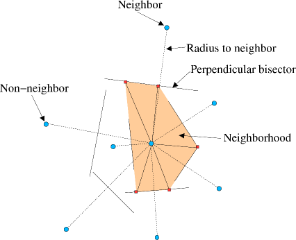
Figure 4: Construction of a 2-D Voronoi cell. See text for discussion.

The Voronoi neighborhood of a one-dimensional piecewise linear manifold (such as a fluxon) embedded in three dimensions is described by a family of spliced fourth-order bivariate polynomials (see, e.g., Preparata and Shamos 2000 and references therein); solving such curves is computationally expensive. We instead approximate the Voronoi neighborhood of each fluxel along the fluxon with a prism extruded along the length of the fluxel, and determine the two-dimensional Voronoi neighborhood in the cross section of the prism. When projected into the cross-sectional plane of a central fluxel, the nearby fluxels appear as points, and the construction is straightforward (as illustrated in Figure 4). A line segment is constructed from the central fluxel to each nearby fluxel, and the perpendicular bisector of each such segment is found. The smallest convex polygon that can be constructed from the bisectors and that also includes the central fluxel is the two-dimensional Voronoi cell of the central fluxel. The fluxels whose bisectors contribute to the shape of the Voronoi cell are the neighbors of the central fluxel, and a list of them is retained. After an initial seeding step, the Voronoi calculation at each relaxation step involves only the neighbors and next-nearest-neighbors from the previous step, speeding the calculation. In any sufficiently large field of points, the average number of edges in each Voronoi cell (and hence neighbors of the central fluxel) converges to 6, so the Voronoi calculation for each cell runs in constant average time and for the entire simulation it runs in $O(n)$ time.

The projection function we use to project each fluxel into the cross-sectional plane is not Cartesian: we find the point on the candidate fluxel that is closest to the central fluxel, project that point into two dimensions, and then multiply the radial distance by the fourth power of the secant of the out-of-plane angle to the candidate, artificially raising the distance to fluxels that are out of the cross-sectional plane. This is a smooth way of selecting the fluxels of most interest – those near the perpendicular plane of the central fluxel. Fluxels that are far out of the plane are projected at a farther distance, so that they are usually not close enough to become neighbors during the cell construction. Fluxels are not permitted to interact with the previous and next fluxel on the same fluxon, because the distance to those fluxels is ill-defined (0/0 discontinuity).

The out-of-plane radial scaling function does not affect relaxation results strongly, provided that it is symmetric and grows fast enough: once a nearby projected fluxel is removed far enough from the origin, it is no longer considered a neighbor and does not affect the local force calculation. The fluxels of interest are those near the perpendicular plane of the central fluxel, and there the scaling function is near unity.

Once the Voronoi geometry is known, the magnetic field still remains to be calculated. We are free to choose any non-pathological distribution of flux within the Voronoi cell, as the cells are by definition smaller than the physical resolution of the model. For analytic convenience, we treat the magnetic field in the Voronoi cell as being in sectorwise angular equipartition: the cells are described as a collection of triangular segments, each of which has uniform magnetic field and each of which has a total amount of flux that is proportional to the angle subtended by the segment. This prevents currents from forming at the boundaries between parallel fluxons (by construction, the field strength is equal on opposite sides of such a boundary), allows current sheets to form between nonparallel fluxons, and yields simple formulas for the average field and the perpendicular field gradient. This assumption yields a simple formula for the field-normalized magnetic pressure force $F_{pn}$:

$$\vec{F}_{pn}=\int_{v}^{v+1}\mathcal{F}_{pn}ds=l\frac{\left\langle\bigtriangledown_{\perp}B\right\rangle}{\left\langle B\right\rangle}=l\sum_{i}\frac{\hat{n_{i}}\Delta\phi_{i}}{\pi r_{i}}$$ (10)

where $\hat{n_{i}}$is the direction to the $i^{th}$ neighbor, $\Delta\phi_{i}$ is the angle subtended by the corresponding edge of the Voronoi cell, $r_{i}$ is the distance of closest approach of the corresponding perpendicular bisector, and $l$ is the length of the line segment from $v$ to $v+1$. The formula works even in the case of open Voronoi cells (which are not closed polygons), because although the field is considered to be identically zero in the open directions, it is nonzero in the closed directions. This prevents the magnetic pressure force from being identically zero on the outermost field lines of the simulation (which usually have open Voronoi cells).

2.3 Grid relaxation to find equilibrium solutions

At each relaxation step, FLUX calculates the field-normalized curvature force at each node, and the pressure force at the center of each fluxel. The pressure forces for the leading and trailing fluxels for each node are averaged together, to produce an average pressure force at the node. The average pressure force, in turn, is added to the curvature force at the node to find a normalized total force. At each relaxation step, all nodes are moved in the direction of the corresponding normalized total force, until a relaxation condition is met. This type of relaxation is similar to the magnetofrictional method (Yang et al. 1986; van Ballegooijen 1999) except that the field line location, rather than local field direction, is being relaxed.

All relaxation codes become proportionally less stable as equilibrium is approached, because the component forces are much larger than their resultant, making the local linearization matrix stiff. To overcome this problem and prevent oscillation around the equilibrium, FLUX scales each node’s relaxation step by the square of the stiffness coefficient $\left(\left|\sum\vec{F}_{j}\right|/\sum\left|\vec{F}_{j}\right|\right)$, where $j$ runs over all component forces in the relaxation (in this case the pressure and curvature forces). Further, although the forces are field-normalized, smaller steps must be taken where the fluxons are close together. Hence, the step law used for FLUX with field-normalized forces is:

$$\Delta\overrightarrow{x_{i}}=\delta\tau\left(\frac{\left|\sum\vec{F}_{j}\right|}{\sum\left|\overrightarrow{F}_{j}\right|}\right)^{2}r_{min,i}\sum\vec{F}_{j}$$ (11)

where $i$ is node number, $j$ runs over all forces included in the relaxation, $\delta\tau$ is a small Eulerian step coefficient in fictitious “relaxation time”, the central fraction is the stiffness coefficient, and $r_{min}$ is the closest-approach distance of the closest neighbor to the following or trailing fluxel of each node. Relaxation continues until the stiffness coefficient falls everywhere below some threshold, or until a maximum number of steps have been taken.

To consider additional forces in the simulation, it is only necessary to calculate the new force at each node at each relaxation step, and add it to the other forces in the relaxation.

2.4 Boundary conditions

The end of each fluxon may be line-tied (end node forced to a particular location; this is the norm on the photosphere), open (end forced at each relaxation step to the surface of a very large sphere), or plasmoid (ends of the fluxon are forced to the same location). With no further consideration for boundary conditions, the fluxon formalism yields free-space boundary conditions, effectively extrapolating the field to infinity in vacuo.

Impenetrable plane-like boundaries with prescribed field normal to the boundary (such as the solar photosphere) are modeled by the method of images: during each Voronoi calculation, each fluxel interacts not only with its physical neighbors but with an image of itself reflected through the plane of the boundary. The reflection is culled in the Voronoi calculation process, just like any other fluxel, so that elements far from the boundary do not interact with it directly. The image fluxel forces edge fluxels to have a voronoi cell boundary coincident with the boundary plane, confining the modeled flux. The field normal to the boundary may be prescribed by tying fluxon end-points to the boundary itself: the pattern is a constant of relaxation, and determines the field in the vicinity of the boundary. If no fluxons are tied to the boundary, then the field normal to the boundary is identically zero.

Formally, there is no magnetic method of images for most curviplanar boundaries. FLUX supports a spherical or cylindrical boundary using a polyplanar (or “disco ball”) approach, in which each fluxel has an image that is reflected through the tangent plane directly under the fluxel’s center. This method works because the only fluxels that interact directly with their reflections are close enough to the surface that the boundary approximates a plane.

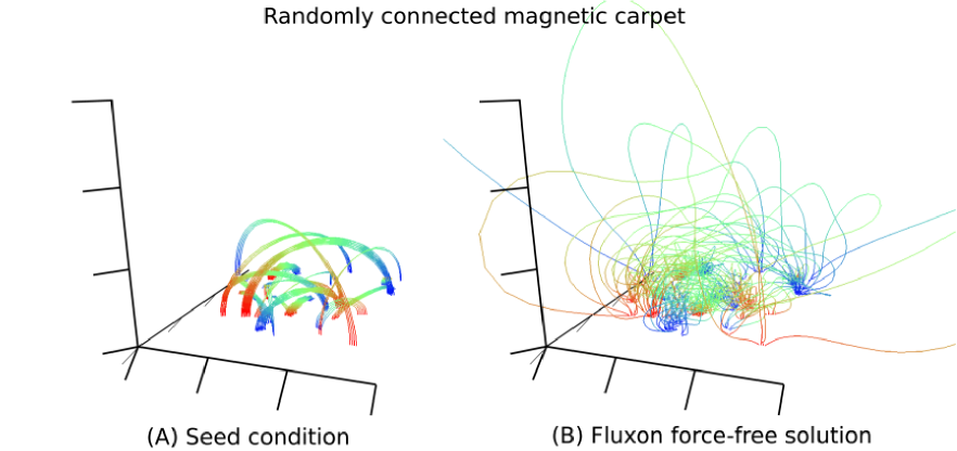
Figure 5: A randomly connected “magnetic carpet” field over a photosphere, calculated with FLUX. The initial field was seeded with a collection of flux concentrations located randomly on a square patch of photosphere. North poles are blue; south poles are red.

2.5 Initial conditions

Because fluxon models explicitly conserve topology, the initial topology map must be specified in advance of the relaxation, in the form of a collection of fluxons that have the correct topology and endpoints, but not necessarily the correct shape; this makes fluxons useful for tracking systems with specified initial topology, such as flare models (e.g. Longcope 1996) or semi-empirical results from tracking of photospheric magnetic features (e.g. DeForest and Lamb 2004). An example initial condition and resulting field solution are shown in Figure 5: an initial collection of fluxons is constructed to represent the connection map and desired topology of the solution, and then relaxed to find the actual magnetic field configuration in the system. To solve quasi-static time dependent problems, one may deform a relaxed solution in a nonphysical way to match updated boundary conditions at the next time step, and then relax to find the new solution.

Fluxon models are less directly suited to solving problems where the initial topology is not known but the full vector field is known at the boundary. In such cases, one must begin with a guessed initial topology, and then use the mismatch between the computed and measured field angle at the boundary as an error function to find the correct topology by trial and error. Alternatively, one may use vector magnetograms to validate topological inferences, for example those derived from magnetic tracking and/or coronal imaging.

2.6 Grid regularization and refinement

Since the shape of the field lines, and not the full position of the nodes, determines the Lorenz force, we are free to impose a nonphysical force along the field to arrange the nodes for optimal sampling. To ensure optimal distribution, FLUX nodes along the same fluxon repel one another with an inverse-square law force, and also are attracted to curvature. This results in a compromise between uniform distribution and clustering near places where curvature is high. Every few hundred relaxation steps, the grid is checked for denseness. Additional nodes are placed wherever the fluxels are longer than the inter-fluxon spacing, and wherever the turn angle at each node is too great. Currently, there is no way to add more fluxons to a model in mid-relaxation, though that type of grid refinement is planned for future work.

2.7 Reconnection

Fluxon models lock in topology, preventing any reconnection that is not inserted explicitly into the model. Because fluxons are represented digitially as linked lists of fluxel locations, it is simple to relink two fluxon lists to achieve discrete reconnection in the model. FLUX supports this capability and offers a programmer interface to relink neighboring fluxons when particular local conditions are met. Planned future work includes studies of current-triggered reconnection in which, once a threshold current density is achieved, reconnection proceeds very rapidly. This behavior is represented by the stick/slip reconnection model of Longcope (1996) and is a possible mechanism for nanoflare heating of the coronal (e.g. Parker 1988).

3 FLUX implementation and performance

FLUX is written in portable C, with a user interface in Perl/PDL (Glazebrook et al., 2003). Initial conditions may be specified either as an initial topology map (non-equilibrium fluxon geometry) or as a collection of potential sources together with boundary tie-points (in which case the code shoots fluxons through the specified potential field from each tie-point). Output is in the form of node coordinate arrays that contain the fluxon geometry and any ancillary data (such as plasma density) indexed by node ID number. The simulation arena is represented as a Perl object that is manipulated using method call syntax. Individual nodes are allocated and freed dynamically. The code can also render fluxon geometry in 3-D using the OpenGL graphics library. Subroutines implementing several forces (both field-normalized and non-normalized) are available in the code, and the user can choose between them at run time. A programmer interface exists for adding more forces into the balance. Initial fluxon configuration and boundary conditions may be specified using the PDL interface.

3.1 Scaling

While developing FLUX we noticed an interesting phenomenon in the code’s scaling properties. The number of nodes required to represent a loop of magnetic flux is dependent on the total amount of curvature in the loop, plus the number of inflection points in the loop. But magnetic fields that are line-tied at the Sun’s photosphere are approximately self-similar against scaling transformations, so that large loops require about the same number of nodes as small loops to represent. The result is that in typical use, FLUX’s memory usage depends almost linearly on the total amount of line-tied flux that is represented, rather than on the total simulation volume. The simulation complexity scales more like a conventional 2-D model than like a 3-D model. We tested this hypothesis with collections of randomly connected “magnetic carpet” fields. One such randomly generated magnetic carpet was shown in Figure 5, in which 40 randomly located flux concentrations have been connected into 20 separate magnetic domains with varying amounts of current. We generated and relaxed 20 carpet models spanning two orders of magnitude in complexity, from 3 flux concentrations to 300 flux concentrations, refining each so that the final vertex angle was limited to 0.25 radian (about $15^{\circ}$) during relaxation by 200 steps of $\Delta\tau=0.2$. We found that the required number of nodes indeed scales as the amount of flux at the boundary over the full range that we tested: more than two orders of magnitude in carpet complexity.

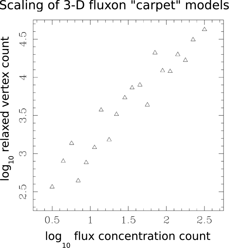
Figure 6: Number of nodes versus number of flux concentrations on the boundary, for a family of magnetic carpet simulations similar to the one in Figure 5. Because of the field’s self-similarity against scaling, the number of nodes scales linearly with the (2-D) complexity of the boundary although the simulations represent the full 3-D field.

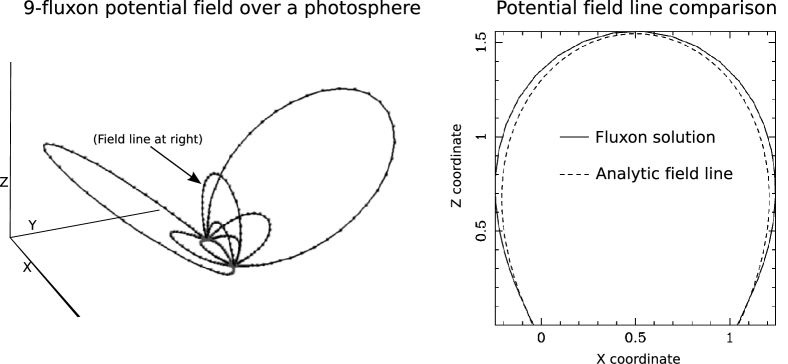
Figure 7: Simple nine-fluxon relaxation reproduces a potential field. LEFT: 3-D rendering of the final fluxon configuration. RIGHT: the central vertical field line closely approximates the shape determined by shooting through an analytic field, as seen in this rendering of the XZ plane. All nine fluxons achieve similar matches in shape.

3.2 Simple validation cases

We demonstrate here that FLUX can reproduce a simple potential field calculation and the behavior of the Lundquist (1950) (linear force-free) and Gold and Hoyle (1960) (nonlinear force-free) flux tubes.

Potential solution

Because FLUX is a full nonlinear force-free field solver, the potential solution has no special properties for testing the code, aside from convenience and ease of representation. We used nine fluxons to connect a square grid of tie points with spacing 0.05, centered at location (0,0,0), to a similar grid at (1,0,0), with a photosphere located in the XY plane. Free-space boundary conditions apply elsewhere than the photosphere, allowing the solution to expand into the positive-Z half-space. Each fluxon’s initial configuration was a single upward jump followed by five horizontal steps and a downward jump (8 nodes per fluxon, including endpoints). The fluxons were relaxed for 1,000 timesteps with $\delta\tau$ set to 0.2, with nodes added periodically to limit the inter-fluxel angle to 0.1 radian (about $6^{\circ}$). The relaxation required about 40 CPU-seconds on a 1.4 GHz Athlon workstation, ending with just under 700 nodes total and an average stiffness coefficient of $8\times 10^{-3}$, indicating good relaxation. The resulting potential field approximation is rendered in Figure 7. The tied line locations approximate the surface penetration of a finite dipole with poles at (0,0,-0.1) and (1,0,-0.1), so we compared the final relaxed shape of each fluxon to the shape of an analytically calculated field line with the same footpoints. The match is quite good, especially considering the coarseness of the model: $\left|\Delta\overrightarrow{B}\right|/B$ between the analytic and fluxon solution is under 8% at every fluxon node, and under 2% everywhere except within 0.05 of the footpoints.

Linear force-free (Lundquist) flux tube

To demonstrate that FLUX is capable of matching analytic force-free solutions that are not potential, we demonstrate convergence to the Lundquist (1950) solution in linear geometry. The Lundquist solution is a cylindrical twisted flux tube along the $z$ axis, with the form

$$B_{z}=B_{0}J_{0}(kr);\,B_{\theta}=B_{0}J_{1}(kr);\,B_{r}=0.$$ (12)

We seeded the solution by shooting fluxons through the analytic Lundquist solution with $k=1$, between the $z=0$ and $z=30$ planes, for $r$ values from $0$ to 10 (near the third node of $J_{1}$). At each $dr$ step in radius, we computed the number of field lines penetrating the $z=0$ plane at that diameter and truncated to the nearest integer, saving the floating-point residual to add at the next $dr$. The integer number of field lines were launched equidistant in $\theta$ around the flux tube, with a phase shift of 2.0 radians at each $dr$. This field line placement has the correct field topology by construction, but is far from correct: chance groupings of field lines in the essentially randomly oriented cylindrical shells dominate variations in field strength.

The resulting paths were inserted into a fluxon model that was relaxed for 300 steps with $\delta\tau$ set to 0.2, with nodes added periodically to limit the inter-fluxel angle to 0.2 radian. Because $\int xJ_{n}^{2}dx$ diverges, the Lundquist flux tube cannot be reproduced with free-field boundary conditions and a finite amount of flux; hence, we applied a low-beta cylindrical boundary at $r=10.05$ during the relaxation: among the neighbor candidates for each fluxel at each time step was an “image fluxel” created by reflecting each of the fluxel’s two vertices through the plane tangent to the cylinder radially outward from the corresponding vertex. This prevented flux tube expansion through the free space around the cylinder, while not directly affecting any flux element in the interior of the modeled tube.

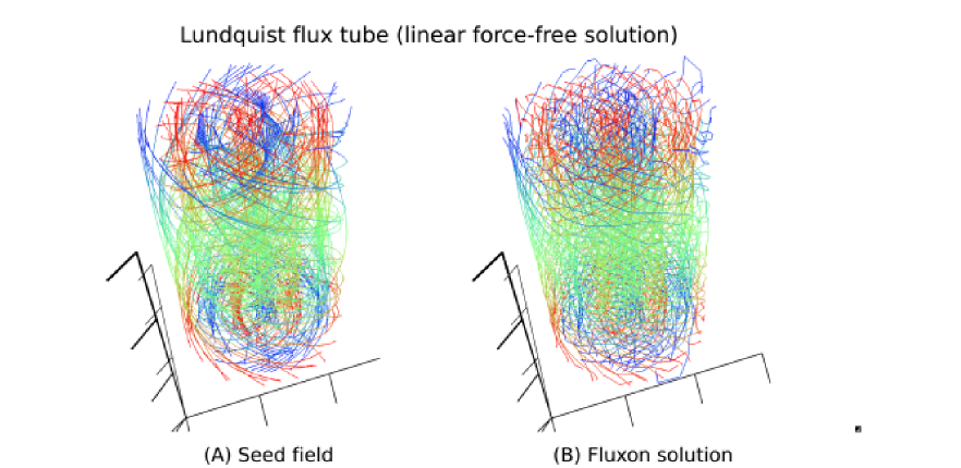
Figure 8: Three-dimensional rendering of the Lundquist flux tube solution with FLUX. Analytically computed field lines were generated and converted to fluxons (LEFT), then perturbed randomly and relaxed with FLUX (RIGHT) in the presence of a cylindrical impermeable boundary. Field line direction is rendered in color, grading from blue at north magnetic poles to red at south magnetic poles.

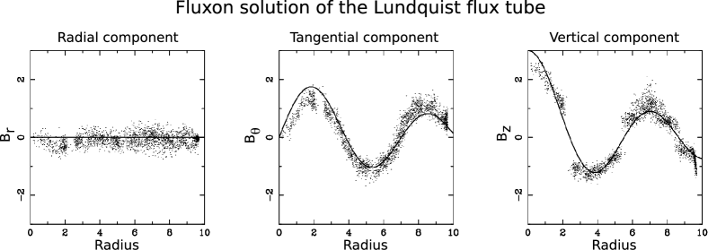
Figure 9: B-field components in cylindrical coordinates at each fluxel center location in the Lundquist flux tube solution in Figure 8. The theoretical values are plotted as solid lines.

The relaxation involved 200 fluxons anchored in 50 concentric rings, consumed about 1000 CPU-seconds, and ended with just over 7,000 nodes and an average stiffness coefficient of $2\times 10^{-2}$ . The resulting approximation of the Lundquist flux tube is rendered in Figure 8. In cylindrical coordinates, the Lundquist solution is dependent only on $r$, the distance from the $z$ axis; hence, to determine the quality of the solution, we produced scatterplots of the calculated field components at each fluxel center in the relaxed solution. Only fluxels in the central third of the solution ($10\leq z\leq 20)$ were considered, to reduce edge effects at the top and bottom of the fluxon system. The scatterplots are shown in Figure 9, demonstrating that the solution has converged to the Lundquist solution. The RMS $\left|\Delta\vec{B}\right|/B$ is 5.4% throughout the volume.

Two features of the plots in Figure 9 require some explanation. First, there is considerable scatter in the plots compared to the potential solution. The scatter is attributable to two separate effects. First, because of the small number of fluxons in each radial sheath, there is some distortion of the field as the fluxons bend one around the other. Secondly, we are representing the field within each fluxon using sectorwise angular equipartition – essentially assuming that the currents are concentrated along the boundaries of triangular prisms around each fluxon – but the Lundquist solution requires a volume current. Increasing the number of fluxons, or using an interpolation technique that averages the field over more than one fluxel, reduces the scatter significantly both by reducing the bending effect and by better approximating a volume current.

Secondly, the $z$ component of the field strength jumps across zero near the nodes of $J_{0},$ rather than passing smoothly through it. This is due to the discrete nature of the fluxons and the construction of our initial seed solution: no fluxons were launched from the rings where $J_{0}=0$, because by construction each ring only contained sufficient fluxons to approximate the total magnetic flux penetrating the ring. Hence our solution develops a small current sheet near each node of $J_{0}$. While better attention to the seed field would reduce this artifact, we have retained it here to point out the care that is required in selecting the initial seed field and fluxon locations. The gaps in the statistical population between $r=2.5$ and $r=5.5$ are due in part to this effect and in part to the periodicity in $r$ of the original seed population of fluxels; this fossil periodicity is more readily apparent in the radial component scatterplot at far left.

While we have plotted field values only at fluxel centers, the field can be calculated anywhere within the simulation volume by interpolating between the field values at nearby fluxels.

Nonlinear force-free (Gold-Hoyle) flux tube

The Gold-Hoyle flux tube has the interesting property that $d\theta/dz$ is constant across field lines. The Gold-Hoyle solution has the form

$$B_{z}=\frac{B_{0}}{1+\mu^{2}r^{2}};\,B_{\theta}=\frac{B_{0}\mu r}{1+\mu^{2}r^{2}};\,B_{r}=0.$$ (13)

which, like the Lundquist solution, carries an infinite amount of flux (the enclosed flux diverges logarithmically in $r$). We tested a Gold-Hoyle-like solution by launching a square, 11x11 array of fluxons from each of two flux concentrations in free space, separated by a distance of 30 on the $z$ axis. The flux concentrations were parallel to the $xy$ plane, and had an inter-fluxon spacing of just 0.1. The total twist was 2.0 turns along the length of the flux concentration. Because the twist is locked in by the fixed topology, this nonphysical initial condition should relax to become a Gold-Hoyle flux tube with the correct amount of twist for its final radius. We allowed it to expand to a radius of 7.5 using zero-normal-field cylindrical boundary conditions. Figure 11 shows the seed field configuration and the relaxed flux tube. We fit compared the fluxon field results to the family of analytic solution by plotting field component values at each fluxel center in the middle third of the simulation volume, and fit the value of $\mu$ by eye to about 0.65. The results are shown in Figure 11.

As with the Lundquist solution, we have plotted the magnetic field value only at fluxel centers. Figure 11 shows a good match between the fluxon result and the analytic solution, with no large current sheets as were demonstrated in the Lundquist flux tube. As above, the periodicity of the fluxon placement is due to the regularity of the initial seed field, but the field strength and direction are close to the analytic value everywhere. The fossil periodicity is much more evident in this solution than in the Lundquist solution, because the regularity of the initial condition ensures less relative movement of the fluxons in finding their equilibrium positions.

The slope of $B_{\theta}$ vs. $r$ is slightly steeper in the fluxon curve than in the analytic solution. We attribute this effect to the vertical expansion of the outermost fluxons outside the intended cylindrical volume, which reduces the amount of twist per unit length in the outer portion of the volume. The effect may be reduced by expanding the source pattern, as in the seed condition for the Lundquist solution, above, or by imposing impenetrable boundary planes above and below the tube.

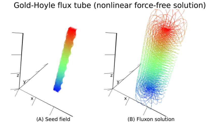
Figure 10: Three-dimensional rendering of the Gold-Hoyle flux tube solution with FLUX. Analytic nonphysical field lines were generated and converted to fluxons (LEFT), then relaxed with FLUX (right) in the presence of a cylindrical impermeable boundary. Field line direction is rendered in color, grading from blue at north magnetic poles to red at south magnetic poles.

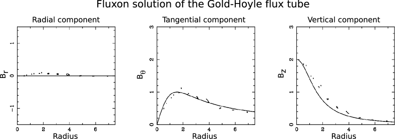
Figure 11: B-field components in cylindrical coordinates at each fluxel center location in the Gold-Hoyle flux tube solution in Figure 10. The theoretical values are plotted as solid lines.

4 Conclusions and future work

We have introduced fluxon modeling and a prototype code, FLUX, that is being released as free software; and have demonstrated that FLUX can reproduce simple potential, linear, and nonlinear force free field solutions. FLUX is currently useful as a magnetofrictional force-free field solver, but it is also intended as a prototype of a much more complete MHD model. FLUX is very promising in two important respects: first, it exactly preserves field topology, potentially yielding a better approximation of ideal MHD than is possible with a conventional Eulerian approach to MHD; and second, it demonstrates good scaling properties that suggest it will perform very well when applied to more complex systems.

We are releasing FLUX as free software that is available as source code for any purpose at all. It may be obtained from the authors, via the web at http://www.boulder.swri.edu/~deforest/FLUX, via Solarsoft Freeland and Handy 1998 as part of the “PDL” package, or via the Community Coordinated Modeling Center Hesse et al. 2002. Future work on FLUX will take two directions: addition and testing of plasma and other forces to study non-force-free equilbria; and addition of dynamic forces to study quasi-stationary MHD systems and, ultimately, full inertial MHD evolution.

References

- Amari and Luciani [1999] T. Amari and J. F. Luciani. Confined Disruption of a Three-dimensional Twisted Magnetic Flux Tube. AP J L, 515:L81, April 1999.
- Antiochos et al. [1999] S. K. Antiochos, C. R. Devore, and J. A. Klimchuk. A Model for Solar Coronal Mass Ejections. AP J, 510:485, January 1999.
- Calidonna and Naddeo [2005] C. R. Calidonna and A. Naddeo. Using a Hybrid CA Based Model for a Flexible Qualitative qubit Simulation. In Conf. Computing Frontiers, page 145, 2005.
- Chen and Shibata [2000] P. F. Chen and K. Shibata. An Emerging Flux Trigger Mechanism for Coronal Mass Ejections. AP J, 545:524, December 2000.
- DeForest and Lamb [2004] C. E. DeForest and D. A. Lamb. Clustering of the Small-Scale Field. BAAS, 204, May 2004.
- Fan and Low [2003] Y. Fan and B. C. Low. Dynamics of CME Driven by a Buoyant Prominence Flux Tube. ASP Conf Ser., 286:347–354, 2003.
- Freeland and Handy [1998] S. L. Freeland and B. N. Handy. Data Analysis with the SolarSoft System. Solar Physics, 182:497–500, October 1998.
- Glazebrook et al. [2003] K. Glazebrook, J. Brinchmann, J. Cerney, C. E. DeForest, D. Hunt, T. Jenness, T. J. Lukka, R. Schwebel, and C. Soeller. The Perl Data Language, v. 2.4.0. Available via the web: "http://pdl.perl.org", 2003.
- Gold and Hoyle [1960] T. Gold and F. Hoyle. M. Not. RAS, 120:89, 1960.
- Hesse et al. [2002] M. Hesse, M. Kuznetsova, L. Rastaetter, K. Keller, A. Falasca, S. Ritter, and P. Reitan. The Community Coordinated Modeling Center: A Strategic Approach to the Transition of Research Models to Operations. AGU Spring Meeting Abstracts, pages B7+, May 2002.
- Lin and van Ballegooijen [2002] J. Lin and A. A. van Ballegooijen. Catastrophic and Noncatastrophic Mechanisms for Coronal Mass Ejections. AP J, 576:485, September 2002.
- Longcope [1996] D. W. Longcope. Topology and Current Ribbons: A Model for Current, Reconnection and Flaring in a Complex, Evolving Corona. Sol. Phys., 169:91, 1996.
- Lundquist [1950] S. Lundquist. Arkiv. Fysik Bd., 2:35, 1950.
- Lynch et al. [2003] B. J. Lynch, P. J. MacNeice, S. K. Antiochos, and T. H. Zurbuchen. Coronal Mass Ejection Breakout with Adaptive Mesh Refinement. AAS/Solar Physics Division Meeting, 34, May 2003.
- Parker [1988] E. N. Parker. Nanoflares and the solar X-ray corona. ApJ, 330:474–479, July 1988. 10.1086/166485.
- Preparata and Shamos [2000] F. P. Preparata and M. I. Shamos. Computational Geometry: An Introduction. Springer, 2000.
- Roussev et al. [2003] I. I. Roussev, T. G. Forbes, T. I. Gombosi, I. V. Sokolov, D. L. DeZeeuw, and J. Birn. A Three-dimensional Flux Rope Model for Coronal Mass Ejections Based on a Loss of Equilibrium. ApJ, 588:L45–L48, May 2003.
- Sturrock [1989] P. A. Sturrock. The role of eruption in solar flares. Sol. Phys., 121:387, 1989.
- Sturrock et al. [1984] P. A. Sturrock, P. Kaufman, R. L. Moore, and D. F. Smith. Energy release in solar flares. Sol. Phys., 94:341–357, September 1984.
- Ustinov et al. [1993] A. V. Ustinov, M. Cirillo, and B. A. Malomed. Fluxon dynamics in one-dimensional Josephson-junction arrays. Phys Rev B, 47:8357–8360, April 1993.
- van Ballegooijen [1999] A. A. van Ballegooijen. Photospheric Motions as a Source of Twist in Coronal Magnetic Fields. Washington DC American Geophysical Union Geophysical Monograph Series, 111:213, 1999.
- Welsch et al. [2004] B. T. Welsch, C. R. DeVore, and S. K. Antiochos. Flux Collision Models of Prominence Formation, or Breaking Up is Hard to Do. BAAS, 204, May 2004.
- Yang et al. [1986] W. H. Yang, P. A. Sturrock, and S. K. Antiochos. Force-free magnetic fields - The magneto-frictional method. AP J, 309:383, October 1986.