Importance of Supernovae at $z<0.1$ for Probing Dark Energy

Abstract

Supernova experiments to characterize dark energy require a well designed low redshift program; we consider this for both ongoing/near term (e.g. Supernova Legacy Survey) and comprehensive future (e.g. SNAP) experiments. The derived criteria are: a supernova sample centered near $z\approx 0.05$ comprising 150-500 (in the former case) and 300-900 (in the latter case) well measured supernovae. Low redshift Type Ia supernovae play two important roles for cosmological use of the supernova distance-redshift relation: as an anchor for the Hubble diagram and as an indicator of possible systematics. An innate degeneracy in cosmological distances implies that 300 nearby supernovae nearly saturate their cosmological leverage for the first use, and their optimum central redshift is $z\approx 0.05$. This conclusion is strengthened upon including velocity flow and magnitude offset systematics. Limiting cosmological parameter bias due to supernova population drift (evolution) systematics plausibly increases the requirement for the second use to less than about 900 supernovae.

I Introduction

Type Ia supernovae (SN) observations discovered the acceleration of the universe perl99 ; riess98 and have proved central in progress elucidating the nature of the dark energy responsible snls ; knop03 ; riess04 . SN provide a clear, direct, and mature method for mapping the expansion history of the universe, $a(t)$, with their measured flux giving the distance and hence lookback time $t$ through the cosmological inverse square law and their redshift $z$ giving the scale factor $a$.

Ground-based SN surveys are already underway to obtain hundreds of SN in the range $z=0.2-0.9$, suitable for measuring an averaged, or assumed constant, dark energy equation of state. Plans are well advanced for a comprehensive SN experiment aimed at accurate determination of dark energy properties including dynamics, in the form of a wide field space telescope exquisitely characterizing some 2000 SN over the range $z=0.2-1.7$, with launch planned by 2013. We consider here what specific low redshift (“local”: $z\lesssim 0.2$) SN program would strengthen either of the higher redshift SN programs, combined with Planck CMB constraints on the distance to last scattering. (We do not consider adding further probes, since it is useful to obtain a answer through purely geometric probes, as well as comparing results from different techniques.)

Just as lh03 ; fhlt brought into sharp relief the importance of SN at $z\gtrsim 1.5$ for probing dark energy, due to their ability to break degeneracies, control systematics, and realistically follow dark energy dynamics, here we show similar crucial roles of SN at $z\lesssim 0.1$. Local SN serve two key purposes: leverage in breaking degeneracies by anchoring the low redshift Hubble, or magnitude-redshift, diagram, and providing a well characterized set of SN to search for systematic magnitude effects through subclassification (“like subsets”). In §II we demonstrate the cosmological need for a low redshift sample, and follow this in §III with detailed analysis of the numbers and redshift distribution for optimum complementarity with the higher redshift SN. Issues of systematics including evolution and intrinsic dispersion are discussed in §IV, and a two stage survey program outlined to fulfill the required science criteria.

II Anchoring the Hubble Diagram

The Hubble diagram plots the calibrated peak magnitude $m$, or flux received, of SN vs. their redshift. Since the magnitude is a convolution of the intrinsic luminosity and the distance, to employ the SN data as a distance probe from which we extract cosmological parameters we need to anchor the diagram at low redshift where the distance becomes independent of cosmology. This serves to constrain the intrinsic luminosity (combined with the Hubble constant) in a nuisance parameter ${\cal M}$.

Also, at low redshift the cosmological information enters first in the form of the deceleration parameter $q_{0}=(1+3w_{0}\Omega_{w})/2$, where $\Omega_{w}$ is the dark energy density in units of the critical density and $w_{0}$ its present equation of state ratio. If we concentrate on the dark energy equation of state plane $w_{0}$-$w_{a}$ where $w(a)=w_{0}+w_{a}(1-a)$, then at low redshift there is no dependence on $w_{a}$ and confidence contours from local SN data would be vertical. As we consider SN at higher redshifts, the contours rotate, with the degeneracy direction eventually achieving

$$3.6\,\Delta w_{0}+\Delta w_{a}={\rm constant}$$ (1)

at $z\gg 1$ (for the flat $\Lambda$CDM case of $w_{0}=-1$, $w_{a}=0$).

For both these reasons, local SN are essential for anchoring the Hubble diagram. We illustrate their use in Fig. 1, showing constraints on dark energy with and without local SN added to higher redshift data. The local SN here comprise 300 SN at $z=0.05$ (we discuss the insensitivity to the redshift distribution later), with statistical magnitude dispersion 0.15 mag and a systematic floor of 0.01 mag (roughly equivalent to expectations for the Nearby Supernova Factory snf ). The sample SN09 corresponds to 500 SN uniformly distributed between $z=0.2-0.9$ with dispersion 0.15 mag and a systematic of 0.04(1+z)/1.9 (roughly equivalent to a completed Supernova Legacy Survey snls ). SN17 has 2000 SN between $z=0.2-1.7$ with roughly constant numbers per cosmic time interval, with dispersion 0.15 mag and systematic 0.02(1+z)/2.7 (roughly equivalent to the SN sample of the future Supernova/Acceleration Probe (SNAP snap )). In all cases we take a flat, fiducially $\Lambda$CDM with $\Omega_{m}=0.28$, universe and include a CMB prior of 0.7% on the distance to last scattering.

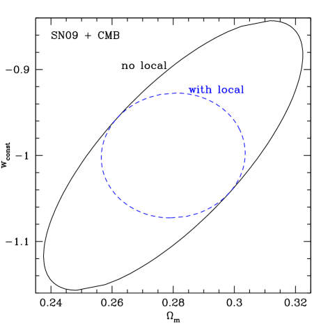
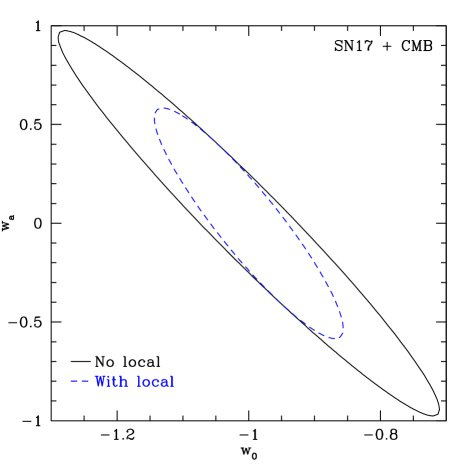
Figure 1: A well controlled low redshift sample of supernova is an essential complement to higher redshift SN experiments. Lack of local SN (here 300 at $z=0.05$) diminish the cosmological leverage by a factor of two on both the matter density and the (assumed constant) dark energy equation of state for a near term SN survey to $z=0.9$ (top panel), or again by a factor two in the equation of state plane for a future SN survey to $z=1.7$ (bottom panel). Contours show $1\sigma$ joint (68%) confidence levels and systematics are included as in the text.

Without the local SN, constraints from the current SN experiments will be a factor of two worse on both $\Omega_{m}$ and an assumed constant equation of state $w_{\rm const}$. For the future SN experiment with tight systematics control to $z=1.7$, the leverage on the dark energy equation of state parameters is approximately a factor of two worse without local SN. Thus it is crucial to implement a properly designed low redshift SN survey in order to realize the capabilities of a SN cosmological probe experiment.

III Numbers vs. Redshift

Given the critical need for a low redshift SN experiment to complement higher redshift data, it is important to craft the appropriate requirements for the local sample to fulfill its role. Here we investigate from a cosmological perspective the optimal criteria for the numbers and redshift distribution of the local SN to strengthen a higher redshift sample, within a Fisher matrix approach. We initially treat this for the experiment extending to $z=1.7$ having the aim of understanding the dark energy properties, through its dynamics. Then we consider this for the current/near term experiment to $z=0.9$, which can only see an averaged, or constant, view of the dark energy equation of state. §IV returns to the issue of requirements by considering the role of the local sample in controlling SN systematics.

III.1 Numbers and leverage

If one thinks of the local SN as providing a prior on the parameter ${\cal M}$ (which is an overstrong view as we will shortly see), then fixing ${\cal M}$ would require an infinite number of SN and the absence of any systematics floor. However, even a perfect determination of ${\cal M}$ does not give an unbounded improvement on the other cosmological parameters. Their estimation uncertainties become

$$\sigma^{2}(p_{j})_{{\rm fix}\ {\cal M}} = \sigma^{2}(p_{j})_{{\rm fit}\ {\cal M}}-(C_{{\cal M}j})^{2}/\sigma^{2}({\cal M})$$ (2)

$$= \sigma^{2}(p_{j})_{{\rm fit}\ {\cal M}}\,(1-r^{2}),$$ (3)

where $C$ is the covariance matrix and $r$ is the correlation coefficient. For the SN17+CMB case, perfect determination of ${\cal M}$ would improve the estimation of $\Omega_{m}$, $w_{0}$, $w_{a}$ by 21%, 70%, 55% respectively. However, as we saw from Fig. 1, a local sample of 300 SN at $z=0.05$, with systematics, already offers substantial improvement, indeed 90%, 71%, 73% of the improvement possible from the unrealistic case of perfect determination without systematics floor.

Furthermore, the effect of a finite sample is even closer to saturating the case of infinite numbers of local SN because local SN do not in fact constrain purely ${\cal M}$. Because they are at finite distances, $z\neq 0$, the local SN have unavoidable covariances mixing ${\cal M}$ and the cosmological parameters. This will further cause a plateau in the numbers of local SN effective in complementing higher redshift SN to impose cosmological constraints.

More and more local SN will not have continuing direct benefit for cosmological constraints. To examine where the point of diminishing returns lies, we consider the definite case of local SN centered at $z_{c}=0.05$. As we will see, this is close to the optimum when the covariance mentioned above and systematics are taken into account, but we emphasize that the saturation is a product of the innate cosmological degeneracy, independent of systematics.

Figure 2 illustrates the saturation of the cosmological constraints as we increase the number of local SN. The uncertainties in $w_{0}$ and $w_{a}$ improve extremely little and far more slowly than the naive $N^{-1/2}$ behavior. For reference, the blue dotted line shows improvement as $N^{-0.1}$. We see that 300 local SN is close to optimum in strengthening the higher redshift SN program. Increasing the local SN numbers beyond 300 does not even attain $N^{-0.1}$ improvement. Indeed, for $N>10^{4}$ the power law index is flatter than $-0.002$; for $N\gg 300$ the improvement over 300 SN is only 5-10%. (And when we take into account below the interaction of the redshift $z_{c}$ with the cosmological degeneracy, the use of $10^{4}$ SN with $z_{c}=0.1$ still provides 10-12% worse constraints than 300 SN with $z_{c}=0.05$.)

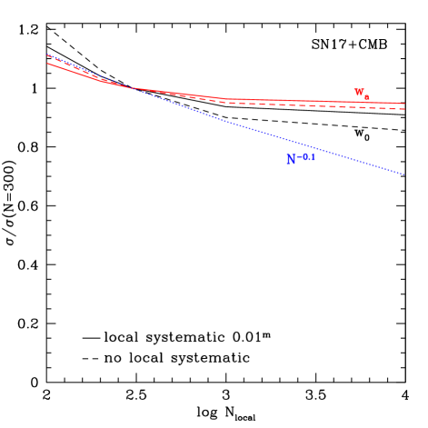
Figure 2: Cosmological parameter estimation is a slow function of the number $N_{\rm local}$ of supernovae in the low redshift sample. (The curves here take $z_{c}=0.05$, but the behavior is similar over $z_{c}=0.03-0.15$.) Due to inherent cosmological degeneracy, the point of diminishing returns is reached near $N_{\rm local}\approx 300$, whether systematics are present (solid curves) or not (dashed curves). The blue dotted curve shows a scaling of $N^{-0.1}$ for comparison.

Overall, there is little direct cosmological use for $N>300$. As we drop below 300 local SN, the degradation is faster than $N^{-0.1}$ for $w_{0}$, and for $w_{a}$ as we drop below 200. Note that this trend remains the same whether we include systematics or not; the saturation is due to the innate and unavoidable cosmological degeneracy. (We have checked that this holds for a reduced intrinsic magnitude dispersion of 0.1 mag as well, though as the ratio of dispersion to systematic level decreases the sample saturates at a slightly smaller size.) Thus, for a homogeneous sample, 300 local SN is close to optimal for cosmological parameter constraints.

III.2 Redshift and leverage

We now examine the optimal redshift location, given the presence of the cosmological degeneracy. Returning to our earlier point about covariance between parameters for a sample at finite redshift, $z_{\rm loc}$, we seek to minimize the degeneracy. To gain an intuitive feeling for this, consider the local SN as determining the magnitude $m(z_{\rm loc})$ to precision $\sigma_{\rm loc}$. This data can be viewed (purely illustratively) as putting a prior on

$$Y\equiv{\cal M}+5\log d_{l}(z_{\rm loc}),$$ (4)

which is added to the Fisher information of the higher redshift SN through

$$F^{\rm prior}_{ij}=\frac{1}{2\sigma_{\rm loc}^{2}}\,\frac{\partial^{2}(Y-\bar{Y})^{2}}{\partial p_{i}\,\partial p_{j}},$$ (5)

where $p_{i}$ are the cosmological parameters. If $z_{\rm loc}\ll 1$ then we can calculate analytically the effect of the prior.

Because the luminosity distance

$$d_{l}(z_{\rm loc}\ll 1)\approx z+(z^{2}/4)[1-3w_{0}(1-\Omega_{m})],$$ (6)

the low redshift SN do not determine ${\cal M}$ but rather constrain a certain combination of ${\cal M}$, $\Omega_{m}$, and $w_{0}$. An unavoidable degeneracy remains, regardless of how many local SN are measured. The cross terms between ${\cal M}$ and the cosmology parameters are proportional to $z_{\rm loc}$ and the cosmology-cosmology terms go as $z_{\rm loc}^{2}$. To minimize the degeneracy, and hence increase the cosmological constraining power, we need to minimize $z_{\rm loc}$ (subject of course to other uncertainty sources such as peculiar velocities, which we address below).

The illustrative analytic expression of Eq. (6) agrees extremely well with the numerical calculations (which we always use), pointing up the inherent cosmological degeneracy that leads to the saturation in the use of large numbers of local SN for cosmological leverage and the preference for lower redshift. Thus, local SN at $z=0.05$ strengthen the higher redshift program much more than SN at $z=0.1$. For example, with 300 local SN, the degradation in constraints if $z_{\rm loc}=0.1$ rather than 0.05 is 24%, 16% for $w_{0}$, $w_{a}$ (and goes roughly linearly with deviation of $z_{\rm loc}$ from 0.05). As already seen, even large numbers of SN at $z_{\rm loc}=0.1$ cannot overcome this disadvantage.

As expected, the cosmological degeneracy imposes a monotonic optimization, pushing $z_{\rm loc}\to 0$. This, however, is impractical for a realistic experiment. Two factors dominate in working against very low redshift: the smaller volume available and hence fewer SN, and uncertainties contributed to the distance determination by random and coherent peculiar velocities. These raise the very low redshift end of the optimization curve, creating a minimum at a finite redshift.

To take into account the volume effect, we realize that an experiment with fixed survey time, centered at $z_{c}$, can amass a number $N$ of well characterized SN (i.e. not just discovered, but followed up with spectroscopy), where

$$N\sim\int_{\rm bin}dz\,z^{2}A(z),$$ (7)

where $A(z)$ gives the dependence on the redshift depth of the solid angle that can be covered in the survey time. This accounts for the increased amount of time required to observe fainter SN. We approximate $A(z)\sim z^{-\gamma}$, which includes the cases of sky noise domination ($\gamma=4$) and source noise domination ($\gamma=2$), and should provide a reasonable fit between these two limits. Both $N$ and $A$ are normalized to the $z_{c}=0.05$ case of 300 well characterized SN in 20000 deg². We limit the sky area to a maximum of 30000 deg² and take the total redshift bin width to be 0.05, centered at $z_{c}$. We have checked that the exact distribution of SN around the central redshift has very weak influence, of order 1% in the parameter constraints, i.e. it does not matter if within the bin the SN are taken to be all at the bin center, uniformly spread, or scaled with the local volume element.

Effects due to peculiar velocities of galaxies in which SN reside consist of a statistical error due to random velocities (which we take to be 300 km/s) and a systematic error due to bulk motions. The latter is treated following the formalism of huigreene ; cooraycaldwell and we approximate their results by an irreducible error across the local redshift bin of $\sigma^{2}_{\rm vsys}\sim A^{\alpha}z_{c}^{-\beta}$, added to the SN random variance. We find a good fit with

$$\sigma_{\rm vsys}=0.0077^{m}\left(\frac{A}{20000\,{\rm deg}^{2}}\right)^{-1/4}\left(\frac{z}{0.065}\right)^{-3/2}.$$ (8)

Putting all this together, Fig. 3 shows the realistic dependence of the cosmological constraints on $z_{loc}$. There is now a clear optimum location for the local SN sample, at $z_{c}=0.05-0.06$, to maximize the science return of the SN experiments. Recall that the true area scaling will lie between the $\gamma=2$ and $\gamma=4$ cases, with $\gamma=2$ (source noise domination) holding for more nearby SN observed near peak brightness and $\gamma=4$ (sky noise domination) holding for more distant SN or observations away from peak brightness. At very low redshift, the ceiling on the area makes the results independent of $\gamma$.

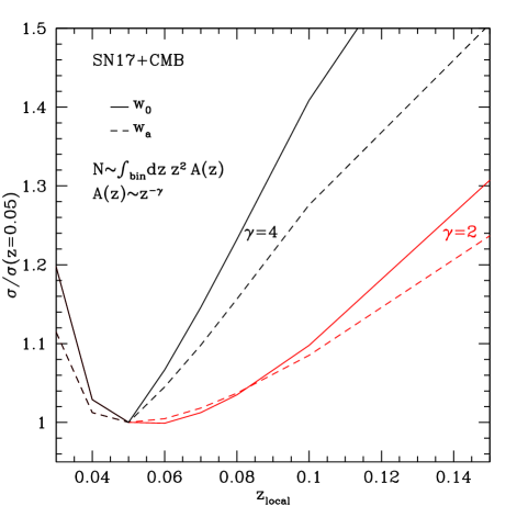
Figure 3: The interaction of cosmological degeneracies, inherent even at low redshift, velocity flow systematics, and observational considerations creates a optimum redshift for the low redshift sample of supernova serving to anchor the Hubble diagram. Here we account for all these effects, with the number of observed supernovae scaling with redshift depth according to the available volume, but also the more limited solid angle $A(z)$ that can be covered in fixed survey time (due to fainter source magnitudes). The optimum central redshift of the low redshift supernovae is $z\approx 0.05$.

Technically, because of the volume weighting, the bin center is not the same as the mean redshift. For example, for a sample spanning $z=0.03-0.08$ (such as the Nearby Supernova Factory), the weighted mean is $\langle z\rangle=0.062$. Interestingly, the standard expression for SN systematics for the SNAP-like sample, $0.02(1+z)/2.7$ (see §II), predicts 0.0079^m here, hence essentially already providing a good approximation to the local sample systematics expressed by Eq. (8).

The conclusion about the optimum $z_{\rm loc}$ remains robust in the presence of a further systematic involving a magnitude offset between the local sample and the higher redshift sample, due to calibration for example. Such a step or offset has long been recognized as a possible observational feature, and treated in both its random and coherent aspects in various analyses such as klmm ; linmiq ; linbias . Considering offsets limited by Gaussian priors of 0.01 or 0.02 mag, we find that this does not change the shape of the curves in Fig. 3 nor the location of the optimum at $z_{\rm loc}\approx 0.05$.

III.3 Matching current supernovae surveys

It is of considerable interest to consider as well the optimization of the nearby sample for complementing ongoing and near term SN experiments that provide data sets similar to the SN09 case of §II, i.e. extending to $z=0.9$. Recall that Fig. 1 showed that the local sample played a crucial role here too. The key cosmological effects and formalism remain the same as in §III.1-III.2.

Figure 4 again illustrates the saturation of cosmological leverage as the number of SN increases. Here we see that 125-150 local SN prove sufficient to serve as the low redshift anchor for the Hubble diagram. The ratio of local:higher redshift SN is now 1:4. The reduced ratio makes sense since for this case we fit only three parameters – ${\cal M}$, $\Omega_{m}$, $w_{\rm const}$. As in the footnote in §III.1, the idealized optimum would be SN distributed in $P$ delta functions in redshift, where $P$ is the number of fit parameters, with one of them at $z\approx 0$. As mentioned there, the inclusion of systematics and priors spreads out the delta functions, reducing the idealized ratio by about a factor of two. Because fewer local SN are involved, diminished intrinsic magnitude dispersion will now have a larger effect; we find that for 0.1 mag dispersion the saturation occurs near 60 local SN.

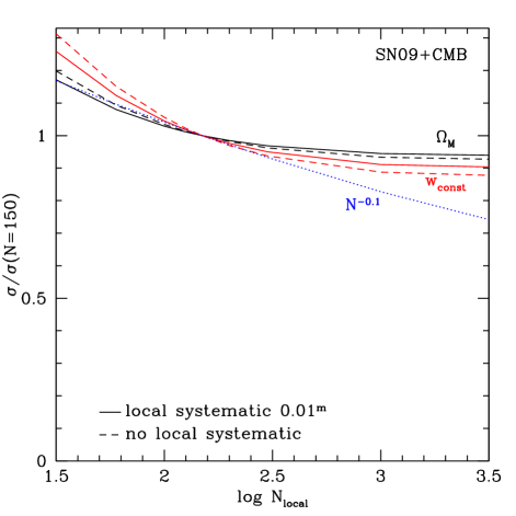
Figure 4: As Fig. 2 but using the higher redshift supernova sample SN09 similar to ongoing surveys (in particular extending to $z_{\rm hi}=0.9$). Diminishing returns in cosmological leverage – now on the matter density $\Omega_{M}$ and constant dark energy equation of state $w_{\rm const}$ – are reached near $N_{\rm local}\approx 125-150$.

The redshift optimization for the local SN remains at $z\approx 0.05$, as illustrated in Fig. 5. The key cosmological influences of innate distance degeneracy and velocity flow systematics are intrinsic to the local sample and so the optimum central redshift for the local SN is insensitive to the higher redshift sample: we again find the optimum is $z_{\rm loc}\approx 0.05$. As before, this remains robust under introduction of a magnitude offset between the local and higher redshift sample.

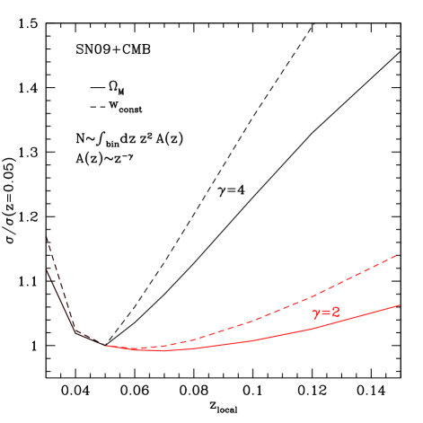
Figure 5: As Fig. 3 but using the higher redshift supernova sample SN09 similar to ongoing surveys (in particular extending to $z_{\rm hi}=0.9$). The optimum central redshift of the low redshift supernovae is $z\approx 0.05$.

IV Subsampling

The second purpose for the local SN program involves identification of SN systematics, characteristics that would break the homogeneity of the sample. Control of such systematics is frequently discussed in terms of subsamples and like vs. like comparison (see, e.g., coping ). Let us estimate the number of local SN required for such subsampling. An important point to be made is that a difference that makes no difference is no difference – and furthermore a difference that cannot be detected is no difference. That is, defining a subset with certain lightcurve and spectral properties distinct from another subset is of limited impact (for cosmology) if they do not differ in their corrected peak magnitudes. Furthermore, a difference in subsample mean magnitudes smaller than the uncertainty from, say, calibration is likewise moot.

IV.1 Population drift

An important issue to begin with, then, is how large a magnitude difference has a substantial cosmological effect. We call subsets, defined on the basis of empirical differences in the lightcurves and spectra, subclasses if they differ in corrected peak magnitude. Subclasses will combine together to determine the mean magnitude at a given redshift; as long as the proportions among subclasses remain independent of redshift there is no cosmological consequence. That is, it is not the presence of subclasses per se, but the population drift and hence weighting in the mean magnitude at each redshift that is important.

Consider the most extreme subclass, subclass 2, lying furthest from the mean magnitude of the other subclasses, collectively subclass 1, in a sort of jackknife test. Suppose its absolute magnitude deviates from the mean absolute magnitude by $\Delta M_{21}$ and it comprises a fraction $f_{2}(z)$ of the total number at redshift $z$. Then the evolution in the mean magnitude relative to the local sample is

$$\Delta M(z)=\Delta M_{21}\,[f_{2}(z)-f_{2}(0)].$$ (9)

Employing the Fisher bias formalism we can calculate the effect of an evolution $\Delta M(z)$ in biasing cosmological parameter extraction. By requiring that the bias on a parameter $\delta p_{i}<0.46\,\sigma(p_{i})$, we ensure that the risk $[\sigma^{2}(p_{i})+\delta p_{i}^{2}]^{1/2}$ degrades the standard deviation by less than 10%. We can then ask what is the largest acceptable $\Delta M_{21}$ for a given population drift function $F(z)=f_{2}(z)-f_{2}(0)$. For each of three forms: $F(z)\sim z$, $1-a$, or $z^{2}$, we find the requirement $\Delta M(z=1.7)<0.016$, for the SN17 case (see the end of this subsection for the SN09 case). This arises mostly from preventing bias in $\Omega_{m}$; for the $z^{2}$ drift the constraints from $w_{0}$ and $w_{a}$ are also comparable, but for the $z$ behavior the next tightest constraint is 0.026 from $w_{a}$, and for the $1-a$ case it is 0.066 from $w_{0}$. So 0.016 mag is a fairly conservative criterion.

The strongest constraint on the observable $\Delta M_{21}$ comes from the most extreme case, where $F(z=1.7)=1$. So we have the requirement of recognizing a subclass with $\Delta M_{21}>0.016$ mag. This is fortunate – if we have a calibration systematic of 0.005 mag then this represents a healthy $3\sigma$ effect. Had the requirement been to distinguish subclasses differing by less than 0.005 we would have been in trouble. We can now flow this down to a requirement on the local SN.

Note that what concerns us is not the evolution as such, but the uncertainty in the evolution. If the population drift is rapid, $f_{2}(z=1.7)\gg f_{2}(0)$, then the magnitude evolution will be insensitive to $f_{2}(0)$. The uncertainty will arise from the precision on knowing $M_{1}$ (the absolute magnitude of the main population) and $M_{2}$, and any correlation (e.g. from calibration). We learn about $M_{1}$ and $M_{2}$ from studying the local sample, where we know the distance. If the dispersions of subsamples 1 and 2 are similar, but population 2 is much rarer, $N_{2}\ll N_{1}$, then the uncertainty on $\Delta M_{21}$ is dominated by the number of local SN in subclass 2.

To determine the mean magnitude of a subclass to 0.016, in the presence of measurement dispersion of 0.15 mag, we need $N_{2}=(0.15/0.016)^{2}=88$ local SN of this subclass.

The results when considering the SN09 case are similar. The requirement on the magnitude drift, or subclass deviation, becomes $\Delta M(z=0.9)=0.019-0.025$; this implies a need for 36-62 local SN of this subclass.

IV.2 Improved standardization

One instance in which a subset that is not a subclass (i.e. does not differ in its mean peak magnitude) can be useful is when the subset exhibits decreased dispersion about the mean, that is, when it is a more standardized candle. Identification of such subsets within the local sample is of interest, and is a positive effect as opposed to the bias caused by drifting subclasses. (However note that explaining the full sample dispersion of, say, 0.15 mag by multiple subclasses of smaller dispersion requires the means of these subclasses to differ.)

The effect of reduced dispersion, in particular of just a subset, may not be dramatic. If 1/3 of the SN have dispersion 0.05 mag rather than 0.15 mag, this only reduces the overall dispersion to 0.126 mag. If the overall dispersion is reduced to 0.1 mag from 0.15 mag, then the equation of state parameters $w_{0}$, $w_{a}$ improve by 15% (for the canonical survey characteristics). Reduced dispersion to 0.1 does not much affect the bias level: the requirement is $\Delta M(z=1.7)<0.015$ for $F(z)\sim z^{2}$ and 0.016 for $F(z)\sim z$, $1-a$. However this does mean that the subclass magnitude can be determined with $(0.1/0.015)^{2}=44$ SN, half the number needed previously. Thus subsets with reduced dispersion can reduce the number of local SN needed to guard against subclass bias, and the numbers of local SN we quote below are therefore conservative.

IV.3 Two stage program

To harvest a subset of size $N_{2}$, which represents a fraction $f_{2}(0)$ of the full population, requires a local sample totaling $N_{2}/f_{2}(0)$. Thus, if the most extreme subclass is also the rarest, we face a challenge. Suppose subclass 2 represented only 5% of SN at $z=0$, but close to 100% at $z=1.7$. Then we would need $88/0.05\approx 1800$ local SN.

To ameliorate the factor 20 increase in numbers, one could possibly design the low redshift SN program to concentrate on the extreme examples. One approach would be first to obtain the cosmological leverage number of 300 SN, then concentrate in a second survey stage on the most extreme subclasses (ones deviating from the mean by more than 0.016 mag) and ensure samples of $\sim$100 SN for them. This would involve much more searching time, but not a large increase in follow up – if the subclass could be recognized without the full set of measurements. If successful, such pruning could keep the total sample to 400-900 SN.

We emphasize that what is important in determining the number of local SN is not the number of subsets, or even subclasses, but the number of extreme ($\Delta M_{21}>0.016$), differentially drifting subclasses. If there is more than one extreme subclass, then this decreases $f_{2}(z=1.7)$, say, below unity, and hence loosens the requirement on $\Delta M_{21}$, changing the definition of extreme. Thus it is not unlikely that only one or two extreme subclasses exist in this sense and hence require a sample of only 100-200 Stage 2 local SN in addition to the Stage 1 foundation program of 300 local SN.

The two stage approach also has the virtue that the initial 300 local SN are likely to prove a sufficient data set by itself for the ongoing/near term higher redshift SN program, even with extreme, differentially drifting subclasses.

V Conclusions

Local supernovae serve critical roles for maximal science return from supernova cosmology experiments – anchoring the Hubble diagram and identifying possible systematics – and failure to supply these data can cost a factor of 2 in cosmology parameter determination. General considerations of cosmology in the form of parameter degeneracies, systematics, and biases impose reasonable and somewhat conservative criteria for a low redshift SN program to match and strengthen a comprehensive, next generation higher SN program: 300-900 SN centered at $z\approx 0.05$. We have tested the robustness of this conclusion by including coherent and random velocity systematics, magnitude offsets, and different intrinsic dispersions.

We propose here a two stage approach to the local sample, with the foundational set composed of 300 well characterized local SN. This data then determines the necessary size for an extension, or second stage, which the arguments presented here suggest may require 100-600 additional SN to control systematic biases. The first stage would likely supply the necessary local set to fully match ongoing and near term SN surveys, which we concluded also are optimized by a local data set centered at $z\approx 0.05$.

Though we used straightforward cosmological considerations, for more detail we could also seek future guidance from SN theory on questions such as maximum expected magnitude evolution, population drift predictions, and characteristics for subclasses, and from calibration and measurement error models and simulations. This detail may be unnecessary and is model dependent. The empirical foundations – from well characterized (i.e. spectroscopic time series measured) SN, not just more SN – will define the relation between subsets and subclasses, and the population distribution (e.g. local percentage of low metallicity SN, differing in the mean magnitude by $X$ mag). The data will be the final arbiter of the sample size required.

To achieve understanding of the physics behind the acceleration of the universe, we need a well designed SN program at $z<0.1$ just as we need a comprehensive SN experiment extending to $z>1.5$. Implementing the criteria derived here should ensure that we reach out into the universe with a firm foundation beneath our feet.

References

- (1) S. Perlmutter et al. 1999, ApJ 517, 565
- (2) A.G. Riess et al. 1998, AJ 116, 1009
-
(3)
Supernova Legacy Survey: http://cfht.hawaii.edu/SNLS
P. Astier et al. 2006, A&A 447, 31 - (4) R.A. Knop et al. 2003, ApJ 598, 102
- (5) A.G. Riess et al. 2004, ApJ 607, 665
- (6) E.V. Linder & D. Huterer, D. 2003, Phys. Rev. D 67, 081303
- (7) J.A. Frieman, D. Huterer, E.V. Linder and M.S. Turner 2003, Phys. Rev. D, 67, 083505
-
(8)
Nearby Supernova Factory: http://snfactory.lbl.gov ;
M. Wood-Vasey et al. 2004, New Astron. Rev. 48, 637 -
(9)
SNAP – http://snap.lbl.gov ;
G. Aldering et al. 2004, astro-ph/0405232 - (10) D. Huterer & M.S. Turner 2001, Phys. Rev. D 64, 123527
- (11) L. Hui & P.B. Greene 2006, Phys. Rev. D 73, 123526
- (12) A. Cooray & R.R. Caldwell 2006, Phys. Rev. D 73, 103002
- (13) A.G. Kim, E.V. Linder, R. Miquel, N. Mostek 2004, MNRAS 347, 909
- (14) E.V. Linder & R. Miquel 2004, Phys. Rev. D 70, 123516
- (15) E.V. Linder 2006, Astropart. Phys. 26, 102
- (16) D. Branch, S. Perlmutter, E. Baron, P. Nugent 2001, in Resource Book on Dark Energy, ed. E.V. Linder [astro-ph/0109070]
-
(17)
http://www.ociw.edu/csp ;
W.L. Freedman et al. 2005, ASP Conf. Proc. 339, 50 [astro-ph/0411176] - (18) http://cfa-www.harvard.edu/oir/Research/supernova
- (19) CCD/Transit Instrument II: J.T. McGraw et al. 2006, SPIE 6267, 126
-
(20)
Essence: http://www.ctio.noao.edu/wproject ;
J. Sollerman et al. 2005, astro-ph/0510026 - (21) http://astro.berkeley.edu/ bait/kait.html
- (22) http://sdssdp47.fnal.gov/sdsssn/sdsssn.html
- (23) http://www.mso.anu.edu.au/skymapper
- (24) http://grad40.as.utexas.edu/quimby/tss