Structure of the near-surface layers of the Sun: asphericity and time variation

Abstract

We present results on the structure of the near-surface layers of the Sun obtained by inverting frequencies of high-degree solar modes from “ring diagrams”. We have results for eight epochs between June 1996 and October 2003. The frequencies for each epoch were obtained from ring diagrams constructed from MDI Dopplergrams spanning complete Carrington rotations. We find that there is a substantial latitudinal variation of both sound speed and the adiabatic index $\Gamma_{1}$ in the outer 2% of the Sun. We find that both the sound-speed and $\Gamma_{1}$ profiles change with changes in the level of solar activity. In addition, we also study differences between the northern and southern hemispheres of the Sun and find a small asymmetry that appears to reflect the difference in magnetic activity between the two hemispheres.

1 Introduction

Seismic data have been successfully used to determine the solar interior structure (e.g., Gough et al. 1996). Departures from spherical symmetry have been less well studied. Among the more detailed studies is one by Antia et al. (2001). This study showed that the solar sound-speed profile is not spherically symmetric, and that it depends on both radius and latitude. Helioseismic determinations of solar structure — both the spherically symmetric and the latitudinally dependent parts — are restricted to the deeper layers of the Sun ($r<0.95R_{\odot}$) because of the limitations of the mode sets that are routinely determined by the Michelson Doppler Imager (MDI) on board the Solar and Heliospheric Observatory (SOHO) and from the ground-based Global Oscillations Network Group (GONG). These data sets provide frequencies for p-modes with degree $\ell\leq 190$ and f-modes with degree $\ell\leq 300$ for the most part, and these low- and intermediate-degree modes are not very useful in determining the structure of the near-surface layers of the Sun. However, the f-modes, which are confined to the outermost layers of the Sun, are more sensitive to rotation than structure, and these provide reliable determinations of solar rotation to fairly shallow depths. Solar rotation and other large-scale flows are known to have a strong latitudinal dependence (e.g., Thompson et al. 1996; Schou et al. 1998); this dependence is also known to show a time variation that is correlated with solar activity (e.g., Schou 1999; Basu & Antia 2000, 2002, 2003; Howe et al. 2000, 2004a). Changes in the latitudinal variation of structure in near-surface regions are, however, difficult to study because of the lack of availability of frequencies for high-degree modes.

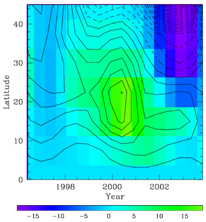
Figure 8: The surface term from the inversions (contours) overplotted on the MAI difference between the higher latitudes and the equator (color image). The MAI difference is in units of Gauss. The surface term units are arbitrary, with solid contours showing positive values and dashed contours showing negative values.

The changes in frequencies of intermediate-degree global modes that are routinely determined from MDI and GONG data show that there are no clearly observable changes in solar structure below $0.95R_{\odot}$ (Eff-Darwich et al. 2002; Basu 2002). There is tentative and indirect evidence that there are indeed solar-cycle related changes in the adiabatic index $\Gamma_{1}$ in the shallower layers of the Sun, around the He II ionization zone, i.e. $\approx 0.98R_{\odot}$, (Basu & Mandel 2004; Verner et al. 2006). Chou & Serebryanskiy (2005) find some marginal evidence for temporal variations near the base of the convection zone, which contradicts earlier negative results (Eff-Darwich et al. 2002; Basu 2002). Similarly, inversions of the frequency splittings of these modes do not show any significant time variations in the latitudinal distribution of sound speed and density below $0.95R_{\odot}$ (Antia et al. 2001, 2003). However, the “surface term” from the inversion (see § 3) changes with time, implying that there could be changes in the structure closer to the solar surface. The surface term also shows a distinct correlation with the distribution of magnetic fields at the solar surface (Fig. 8 of Antia et al. 2001). This leads us to believe that we may be able to detect changes in the structure of the outer layers of the Sun associated with magnetic activity changes by using frequencies of high-degree modes. It is already known that frequencies of high-degree modes vary with local magnetic field strength (e.g., Hindman et al. 2000; Rajaguru et al. 2001; Howe et al. 2004b), and in principle, these frequency differences can be inverted to infer corresponding variations in solar structure or other properties. Earlier studies have shown that the profiles of sound speed and $\Gamma_{1}$ in regions of high magnetic activity differ from those in quiet regions (Kosovichev et al. 2000, 2001; Basu, Antia & Bogart 2004). These studies show that for magnetically active regions, sound speed and adiabatic index $\Gamma_{1}$ are lower than that of quiet regions in the immediate sub-surface layers (about the outer seven Mm or so).

If there are indeed changes in the outer layers of the Sun, we need frequencies of high-degree modes to detect these changes. Unfortunately, it is very difficult to determine the frequencies of very high degree modes through global analysis (e.g., Korzennik et al. 2004 and references therein) and as a result neither GONG nor MDI provide data on high degree modes as standard products, and frequency sets with high-degree modes are not available for different epochs. High-degree solar modes ($l\geq 150$) which are trapped in the outer parts of the solar envelope have lifetimes that are much shorter than the sound travel time around the Sun and hence the characteristics of these modes are mainly determined by the average conditions in the local neighborhood rather than those of the entire sphere. The properties of these modes are better determined by local helioseismic techniques. Ring-diagram (plane-wave $k$–$\nu$) and time-distance analysis (Duvall et al. 1993) are examples of such local helioseismic techniques. Frequencies obtained from ring-diagram analysis have been successfully used to determine the difference in structure between active and quiet regions of the Sun (Basu, Antia & Bogart 2004).

Since high-degree global-mode data are not standard products of the GONG or MDI projects, we use a ring-diagram analysis to obtain solar oscillation frequencies of different latitudinal zones of the Sun at different times. This technique allows us to do a differential analysis of the structure between different regions. We use these frequencies to determine the differences in structure between the equator and higher latitudes. Since we are interested in the near-surface layers where ionization occurs, we need to invert for both the sound speed ($c$) and the adiabatic index ($\Gamma_{1}$) in order to be able to interpret the results, since any temperature change in the ionization zone will also change $\Gamma_{1}$ there. To study how the latitudinal dependence of structure changes with time and activity, we analyze several epochs corresponding to different solar activity levels. The differences in structure between the equator and higher latitudes are expected to be less than those found between strong active regions and quiet regions, because of the smaller differences in the zonally averaged magnetic fields, nevertheless we expect the differences to be detectable.

The rest of the paper is organized as follows: In § 2 we discuss the analysis technique and the regions studied; we give a brief description of the inversion process in § 3; we describe and discuss our results in § 4, and state our conclusions in § 5.

2 Data Analysis

The basic data set consists of the full-disk Dopplergrams obtained by the MDI instrument. Ring diagrams (Hill 1988) are three-dimensional (3D) power spectra of short-wavelength modes in a small region of the Sun. High-degree (short-wavelength) modes can be approximated as plane waves over a small area of the Sun as long as the horizontal wavelength of the modes is much smaller than the solar radius. Ring diagrams are obtained from a time series of Dopplergrams of a specific area of the Sun that are usually tracked with the mean rotation velocity. The 3D Fourier transform of this time series gives the power spectra. These power spectra are referred to as ring diagrams because of the characteristic ring-like shape of regions where the power is concentrated in cuts of constant temporal frequency, reflecting the near azimuthal symmetry of the power in $\bf k$ space. A detailed description of the ring-diagram technique is given by Patron et al. (1997) and Basu et al. (1999). Ring-diagram analysis has the advantage over global-mode analysis that it can be used to study both the non-axisymmetric component of the structure and dynamics of the Sun, as well as the anti-symmetric component of these quantities between the solar northern and southern hemispheres.

For this work we have chosen to analyze MDI Doppler data from eight complete Carrington rotations. The time intervals chosen were dictated by the times at which MDI was in its “Dynamics Program” observing mode, for which full-disc Dopplergrams at a one-minute cadence are available nearly continuously (at duty cycles of at least 85%) over periods as long as the analysis interval, in this case at least one full Carrington rotation. The data intervals selected are listed in Table 1, which also gives the average radio flux at 10.7 cm, a measure of the level of solar activity, during each analysis period.

The data used were not tracked at the photospheric rotation rate as in usual ring-diagram analysis. Instead, they were untracked in the sense that the longitudes were referred to the central meridian of each observation. Corrections were made, however, for the drift of the spacecraft in heliographic latitude over the course of the analysis periods. The analysis interval in each case was 39,936 minutes ($24\times 1664$ min), centered on the time of central meridian crossing of Carrington longitude $180^{\circ}$ of the appropriate rotation as viewed from SOHO. (For CR 2009, the analysis interval was centered on the central meridian crossing of longitude $240^{\circ}$, about 4.5 days before the middle of the rotation, in order to take better advantage of the most complete data coverage from MDI.) For each Carrington rotation we analyzed thirteen latitude bands, each of width $15^{\circ}$, and with a spacing of $7.5^{\circ}$, from $45^{\circ}$S to $45^{\circ}$N. By comparing the results with those obtained using tracked data averaged over the entire Carrington rotation, we have verified that the results are not significantly affected. The untracked regions give us higher frequency resolution because of their longer duration.

Since magnetic activity is a largely local phenomenon, we have calculated the value of the “Magnetic Activity Index” (MAI) of each set to give us a measure of the magnetic activity in each latitude zone. The 10.7 cm radio flux on the other hand is related to total activity averaged over the entire visible hemisphere. The MAI is calculated by integrating the unsigned magnetic field values within the same regions and over the same intervals used to calculate the power spectra, using available 96-minute MDI magnetograms. This index is a measure only of the strong field (fields less than 50 Gauss are set to zero to avoid contamination by zero-level errors and residual noise). The same temporal and spatial apodizations were used. Details of how the MAI is calculated are given by Basu et al. (2004). The MAI’s show the usual butterfly diagram pattern, and their values range from a minimum of 0.3 G to a maximum of about 24 G.

The highly elliptical untracked ring spectra were fitted using the same 13-parameter fit we have used for tracked ones (Basu & Antia, 1999), with suitable adjustments for the very large values of the $U_{x}$ parameter reflecting the advection of the waves by solar rotation in addition to local proper motion.

3 Inversion Techniques

Inversion for solar structure is complicated because the problem is inherently non-linear. The inversion generally proceeds through a linearization of the equations of stellar oscillations, using their variational formulation, around a known reference model (see e.g., Dziembowski et al. 1990; Däppen et al. 1991; Antia & Basu 1994; Dziembowski et al. 1994, etc.). The differences between the structure of the Sun and the reference model are then related to the differences in the frequencies of the Sun and the model by kernels. Nonadiabatic effects and other errors in modeling the surface layers give rise to frequency shifts (Cox & Kidman 1984; Balmforth 1992) which are not accounted for by the variational principle. In the absence of any reliable formulation, these effects have been taken into account in an ad hoc manner by including an arbitrary function of frequency in the variational formulation (Dziembowski et al. 1990).

The fractional change in frequency of a mode can be expressed in terms of fractional changes in the structure of model characteristics, for example, the adiabatic sound speed $c$ and density $\rho$, and a surface term. The frequency differences can be written in the form:

$${\delta\nu_{i}\over\nu_{i}}=\int_{0}^{R_{\odot}}K_{c^{2},\rho}^{i}(r){\delta c^{2}(r)\over c^{2}(r)}\;{\rm d}r+\int_{0}^{R_{\odot}}K_{\rho,c^{2}}^{i}(r){\delta\rho(r)\over\rho(r)}\;{\rm d}r+{F_{\rm surf}(\nu_{i})\over I_{i}}$$ (1)

(e.g., Dziembowski et al. 1990). Here $\delta\nu_{i}$ is the difference in the frequency $\nu_{i}$ of the $i$th mode between the data and the reference model, where $i$ represents the pair ($n,l$), $n$ being the radial order and $l$ the degree. The kernels $K_{c^{2},\rho}^{i}$ and $K_{\rho,c^{2}}^{i}$ are known functions that relate the changes in frequency to the changes in the squared sound speed $c^{2}$ and density $\rho$ respectively, and $I_{i}$ is the mode inertia. Instead of $(c^{2},\rho)$, other pairs of functions may be used, such as density and adiabatic index $\Gamma_{1}$. The term $F_{\rm surf}$ is the “surface term”, and takes into account the near-surface errors in modeling the structure. This term also contains contributions from the very shallow layers of the Sun that cannot be probed by the mode set used.

In this work we determine the relative differences in the squared sound speed, $\delta c^{2}/c^{2}$, and the adiabatic index $\delta\Gamma_{1}/\Gamma_{1}$, as functions of depth, between the solar equator and higher latitudes. In order to minimize systematic errors in the structure inversions, we invert the frequency differences between different parts of the Sun, rather than frequency differences between a region of the Sun and a solar model. To study the latitudinal structure we study differences in solar structure between the higher latitudes and the equator. The main reason for inverting the differences between two sets of solar frequencies is that the structure of the Sun could differ by a very large amount from solar models in the near-surface regions. There are usually many assumptions involved in obtaining the near-surface structure of a solar model, such as the use of the mixing-length formalism to treat convection, the diffusion approximation to treat radiation, and ignoring turbulent pressure; these usually break down close to the surface. Modeling errors may result in large differences in structure between the models and the inverted data in the near-surface layers, and these differences are not always in the linear regime. As a result, Eq. 1 may not hold, and its use could result in systematic errors. The differences between the structure at different latitudes, on the other hand, are expected to be small, and we can thus use Eq. 1 without introducing systematic errors in the results. Another reason for doing a differential analysis is that the non-uniformities in the MDI image geometry are not the same in all Dynamics campaigns. The errors due to these changes are reduced when contemporaneous frequencies are subtracted and used in Eq. 1. Also, the analysis technique itself involves certain approximations. Since the spherical solar surface layers are modeled as being plane-parallel, subtracting the mode frequencies removes some of the geometric errors common to both sets of frequencies. Of course we still need to use a solar model to determine the kernels for the inversion.

Equation (1) constitutes the inverse problem that must be solved to infer the differences in structure between the solar equator and higher latitudes. It can be inverted using a variety of techniques. We carried out the inversions using the Subtractive Optimally Localized Averages (SOLA) technique (Pijpers & Thompson 1992; 1994) and the Regularized Least Squares (RLS) technique. Details of how SOLA inversions are carried out and how various parameters of the inversion are selected were given by Rabello-Soares, Basu & Christensen-Dalsgaard (1999). Details on RLS inversions and parameter selections were provided by Antia & Basu (1994) and Basu & Thompson (1996). Given the complementary nature of the RLS and SOLA inversions (see Sekii 1997 for a discussion), we can be more confident of the results if the two inversions agree.

It must be noted that the kernels used in the inversions were derived in the absence of magnetic field effects. In regions with magnetic fields, there are two ways frequencies can change. One is through the direct effect of magnetic fields on the waves, i.e., through the additional restoring force provided by the field; the second is through the change in structure caused by the magnetic field. The magnitude of these effects depends on the strength and orientation of the magnetic field. To order of magnitude, the relative change in frequency, or the effective squared wave speed, can be expected to be of the order of $v_{A}^{2}/c^{2}$, where $v_{A}$ is the Alfvén speed. Without any additional information it is not possible to distinguish between the direct effect on frequencies of the magnetic field and the indirect effect through modification of the structure.

4 Results

4.1 Frequency differences

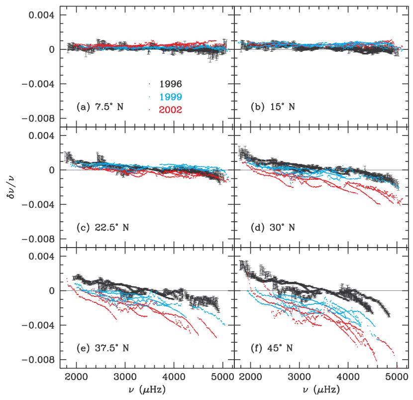
Figure 1: The frequency differences between the equator and higher latitudes in the northern hemisphere of the Sun for three different epochs. The epochs are labeled by calendar year. The differences are in the sense (Higher latitude $-$ Equator). For the sake of clarity, the error bars are plotted for only one set; they are similar for the other sets.

Our results show clear frequency differences between the higher latitudes and the equatorial region of the Sun. We also find that these differences change with time. Fig. 1 shows some of the frequency differences between different northern latitudes and the equator for three Carrington rotations in different years. The frequency differences are significant in all cases. Similar results are seen for other years, and also for latitude zones in the southern hemisphere.

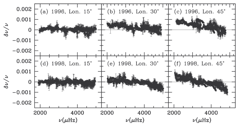
Figure 2: The frequency differences between regions on and off central meridian at the solar equator at two different times. The averages of the differences for both east and west longitudes is shown for each separation. Although there are some systematic effects, they are small compared to the latitudinal differences shown in Fig. 1 (note the scale difference).

Since we find fairly substantial latitudinal effects, it is important to examine possible systematic errors: we expect systematic errors in the frequencies obtained from high-latitude ring spectra due to purely geometric projection effects. This effect should also be present in frequency differences between regions along the equator but at different longitudes with respect to the disk center (neglecting smaller effects due to the non-zero latitude of the observer), and we can use this fact to assess the influence of projection effects on the mode frequencies. If we assume that all the frequency differences between higher-latitude regions and the equator are a result of projection effects, we should find similar frequency differences between the disc center and regions on the equator but away from the disc center, i.e., at different central-meridian longitudes. In order to test this, we determined the frequency differences between the central meridian and other longitudes at the solar equator, i.e. at different positions with respect to the central meridian. For this purpose we analyzed two sets of quiet-Sun data, one from 1996 (CR 1910) and the other from 1998 (CR 1932). The data analysis was similar to that described in § 2. The power spectra for all regions were constructed from 39,936 minutes of data, and hence each power spectrum covered data for the same time interval and the same integrated latitude band on the Sun, but at different angles to the line of sight. In the absence of projection effects we would expect the frequencies at zero longitude (the central meridian) to be the same as those at other longitudes. We did find systematic differences between the higher longitude sets and the zero longitude set, which show similar trend as that for the different latitude zones, with the largest differences being for the maximum longitude separation of $45^{\circ}$; they can be seen in Fig. 2. But we also see that the frequency differences in longitude are much smaller than those in latitude shown in Fig. 1. Thus, we can be reasonably confident that the observed frequency differences between different latitudes and the equator are not simply due to projection effects.

4.2 Radial Dependence of the Results

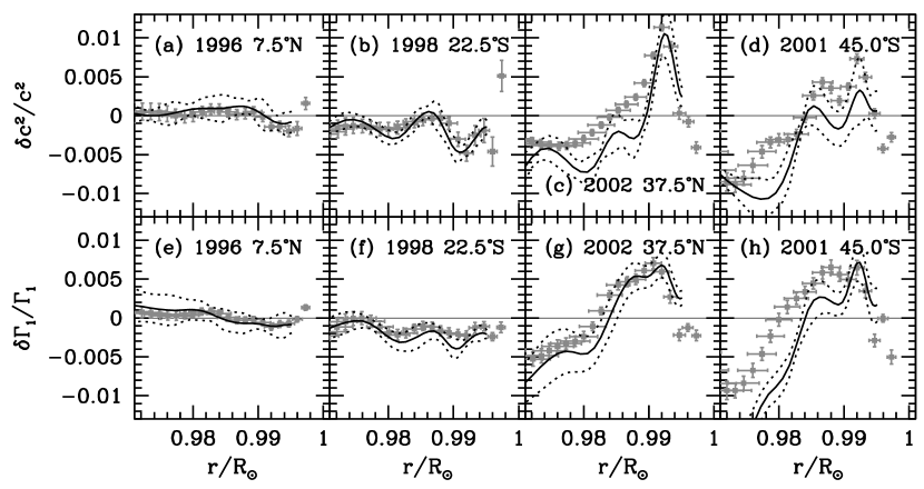
Figure 3: Sample of the inversion results for differences in sound speed and adiabatic index $\Gamma_{1}$ for selected data sets. Each panel is labeled by the year of the data set and the latitude being compared with the equator. The gray points are SOLA results; the vertical error bars correspond to $1\sigma$ errors, and the horizontal error bars are a measure of the resolution of the inversions. The continuous lines are RLS results with the dotted lines showing the $1\sigma$ errors. All the differences are in the sense (Higher latitude $-$ Equator).

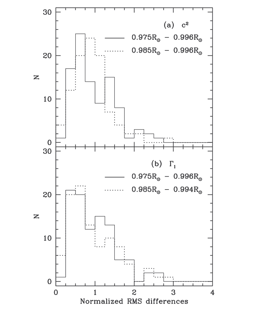
Figure 4: Histogram of the RMS differences between SOLA and RLS inversion results normalized to the errors. Panel (a) shows $c^{2}$ results and Panel (b) the $\Gamma_{1}$ results.

The frequency differences between the higher latitudes and the equator were inverted to determine the corresponding differences in structure. The inversion results are reliable over the radius range $0.975$–$0.996R_{\odot}$, but are most reliable in terms of stability with respect to changes in inversion parameters between $0.985$ and $0.995R_{\odot}$. A sample of the results is shown in Fig. 3. Note the agreement between SOLA and RLS inversions. We find that in most cases the two inversions give the same results within the errors. There are some differences for a few high-latitude cases, but the agreement is generally good. In order to quantify the differences between the SOLA and RLS results, we have determined the root-mean-squared (rms) differences, normalized by the errors, between them. Figure 4 shows the histograms of the differences for the radius ranges $0.975$–$0.996R_{\odot}$ and $0.985$–$0.994R_{\odot}$. The distributions are consistent with random noise.

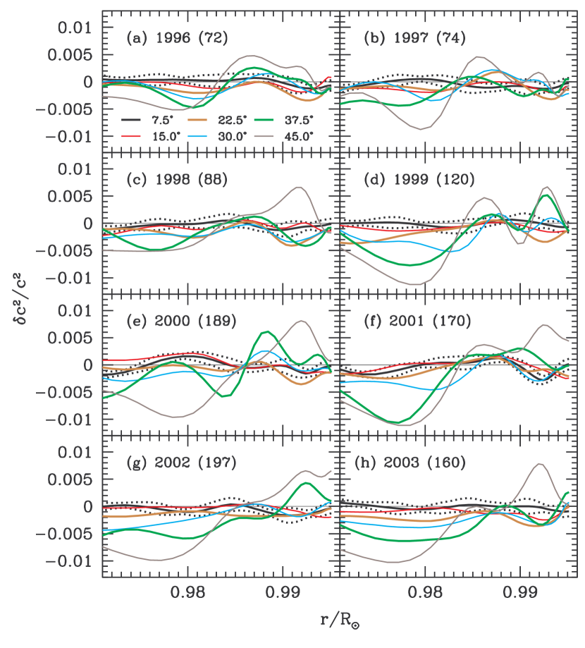
Figure 5: The north-south averaged relative differences in the squared sound speed $c^{2}$ between the higher latitudes and the solar equator, plotted as a function of depth for the eight periods analyzed. Only RLS results are shown; SOLA results are similar. The dotted lines are $1\sigma$ errors. For the sake of clarity, the errors are shown only for the latitude of $7.5^{\circ}$. All differences are in the sense (Higher latitude $-$ Equator). The panels are labeled by the calendar year of the data sets, the numbers in parentheses being the 10.7 cm radio flux in units of SFU for the corresponding period.

The inversion results show that for all the epochs studied, there are considerable differences in sound speed between the solar equator and the higher latitudes. The averages of the northern and southern hemisphere results are shown in Fig. 5. The solar sound speed varies as a function of latitude at all epochs, though it appears that its latitudinal dependence also varies at different epochs. The largest differences are seen for the latitude of $45^{\circ}$, followed by $37.5^{\circ}$. These latitudes generally have a higher sound speed than the equator, particularly above about $0.985R_{\odot}$ or so. There are some signs that the trend is altered closer to the surface.

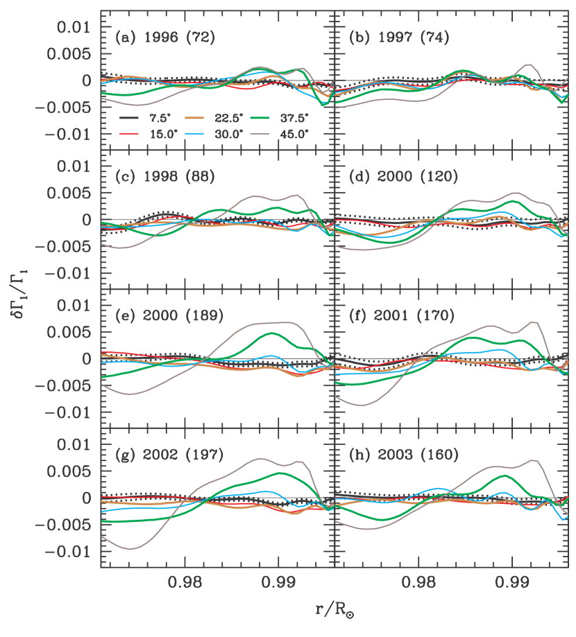
Figure 6: The north-south averaged relative differences in the adiabatic index $\Gamma_{1}$ between the higher latitude and the solar equator as a function of depth for different analysis sets. The same remarks about error bars and labels for Fig. 5 apply.

The $\Gamma_{1}$ differences between the equator and higher latitudes displayed in Fig. 6 also show a trend similar to the sound-speed differences, with larger values of $\Gamma_{1}$ at higher latitudes than the equator. In the case of $\Gamma_{1}$, these differences are more pronounced, and we can also perceive a clear trend with time. The differences between the equator and the higher latitudes appear to increase with the level of solar activity. This is discussed further in § 4.4.

If we concentrate on the structural changes that can be caused by the presence of magnetic fields, we find that it is relatively easy to change the sound speed: it can change if the gas pressure, temperature, or the mean molecular weight $\mu$ changes. Gas pressure changes in response to the additional magnetic pressure, the total pressure $P_{\rm tot}$ satisfying hydrostatic equilibrium conditions being the sum of the gas pressure and magnetic pressure, so that gas pressure decreases when magnetic fields are present. Changing the adiabatic index $\Gamma_{1}$ is difficult, however. It is determined by the equation of state, and is expected to be close to 5/3 except in the ionization zones, where it is lower. Merely changing pressure, density $\rho$ or temperature $T$ does not change $\Gamma_{1}$ everywhere. Changes in $\Gamma_{1}$ can be caused by shifts in the positions of the ionization zones due to changes in the temperature profile. But as pointed out above, magnetic effects are not manifested only by changes in thermal structure. Frequency shifts also occur because of the direct effect of magnetic fields in changing the restoring forces. Part of the observed frequency shifts could be mistakenly interpreted as changes in $\Gamma_{1}$ and $c^{2}$, since the inversion kernels do not take the direct effect of the magnetic fields into account.

Estimating the change in temperature from the changes in $c^{2}$ and $\Gamma_{1}$ is not straightforward. For an ideal gas, changes in $c^{2}$ and $\Gamma_{1}$ are related by

$${\delta c^{2}\over c^{2}}-{\delta\Gamma_{1}\over\Gamma_{1}}=\delta\ln{T\over\mu}.$$ (2)

In the deeper layers of the Sun the gas is fully ionized, hence $\Gamma_{1}$ and $\mu$ are constant, and changes in $c^{2}$ can be related directly to changes in $T$. But the state in the ionization zones is more complicated. Ionization causes both $\mu$ and $\Gamma_{1}$ to change, and hence it is not straightforward to use the above equation to relate changes in $c^{2}$ and $\Gamma_{1}$ to changes in temperature. The estimation of temperature perturbations is hampered by the fact that in the ionization zones, changes in $T$ will give rise to non-zero changes in $\mu$. We have no way to directly determine changes in $\mu$. We could of course estimate how much $\mu$ would change for a given change in $T$ using solar models or the detailed equation of state. But even though we may not be able to use the perturbations in $c^{2}$ and $\Gamma_{1}$ to determine the temperature changes easily, we know that they are always related by

$${\delta c^{2}\over c^{2}}-{\delta\Gamma_{1}\over\Gamma_{1}}=\delta\ln{P\over\rho}.$$ (3)

Thus the difference between the changes in $c^{2}$ and $\Gamma_{1}$ is still a significant quantity.

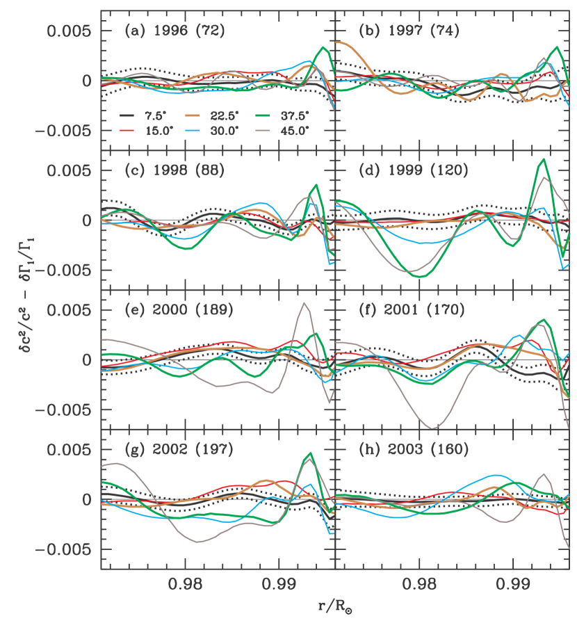
Figure 7: The north-south averaged relative differences in the inferred thermal parameter $c^{2}/\Gamma_{1}$ ($P/\rho$). as a function of depth. The error bars and labels are as described in Fig. 5.

Figure 7 shows the differences between the $c^{2}$ and $\Gamma_{1}$ perturbation profiles. We see that the $\Gamma_{1}$ differences do not account for all the sound-speed difference, thus $P/\rho$ must change as well. The errors in the results are substantial. Nevertheless, we can see that at the high activity epoch, the profile variations are significant at high latitudes.

4.3 The surface term

Global-mode inversions for asphericity showed that the surface term of the inversions follow the pattern of the surface magnetic field (Antia et al. 2001). We have therefore, looked into how the surface term varies with MAI, our local magnetic field index. In Fig. 8 we show surface term contours overplotted on $\delta{\rm MAI}$, the MAI difference between the different regions studied and the equator. Note that the surface term is positive for positive MAI differences (i.e., when the magnetic field of the region is higher than that of the equator), and negative when the MAI difference is negative. However, the linear correlation coefficient of the surface term with MAI difference is not very high, it is 0.38 when all data sets are used, but rises to 0.86 when only sets with $|\delta{\rm MAI}|>5$ G are used. The fact that there is still a good correlation implies that there are changes in layers shallower than those we can resolve in this investigation.

The surface term also correlates with the global activity index. In particular, surface term from high-latitude inversions show a negative correlation with the 10.7 cm flux, while those from low latitudes show a positive correlation. The correlation coefficient at latitude of $30^{\circ}$ and higher is $-0.75$. The coefficient for $15^{\circ}$ and lower is $0.45$, the lower absolute value of the correlation is probably due to the fact that the magnetic field at the equator changes too as activity increases. Since we are doing a differential study with respect to the equator, and because the equatorial and the low-latitude surface terms behave the same way, the overall effect is reduced.

4.4 Dependence of structure on latitude, time, and activity

4.4.1 Asphericity of structure

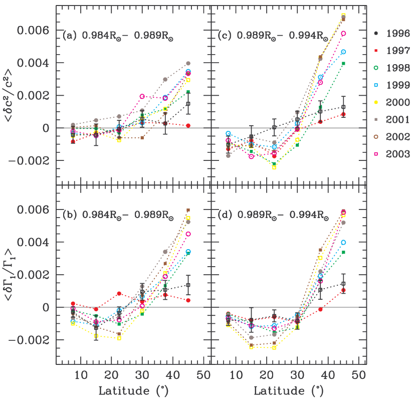
Figure 9: The averaged sound-speed and $\Gamma_{1}$ differences plotted as a function of latitude. Panels (a)–(b) are the averages over the depth range $0.984$–$0.989R_{\odot}$, while panels (c)–(d) are averages over the range $0.989$–$0.994R_{\odot}$. Error bars are shown for the 1996 results; they are comparable in other years. The points are connected to guide the eye.

In order to better determine the dependence of the results on latitude, we concentrate on the averaged results in the radius ranges $0.984$–$0.989R_{\odot}$ and $0.989$–$0.994R_{\odot}$. Fig. 9 shows the averaged results for the two ranges plotted as a function of latitude. We can see very clearly that for the highest latitudes studied ($37.5^{\circ}$ and $45^{\circ}$) both sound speed and $\Gamma_{1}$ are always higher at the higher latitudes than at the equator. At intermediate latitudes they are generally lower than at the equator. This behavior is seen most clearly in $\Gamma_{1}$. At low latitudes (below $30^{\circ}$), $\Gamma_{1}$ is consistently lower than that at the equator, while it is higher at latitudes above $30^{\circ}$. At $30^{\circ}$, the results vary depending on the radius range and the epoch. The behavior of the sound speed differences is a bit more complicated, though in the outer radius range sound speed and $\Gamma_{1}$ behave in a similar manner. In all cases there appear to be strong variations with time, with the differences increasing during epochs of higher solar activity. The difference is particularly clear for $\Gamma_{1}$. The $\Gamma_{1}$ differences become more negative below $30^{\circ}$ with time as solar activity increases, while the differences above $30^{\circ}$ become more positive. The decrease in $\Gamma_{1}$ in the outer layers at low latitudes is what we would expect if the strength of magnetic fields increased there; this is indeed what happens as the solar cycle progresses.

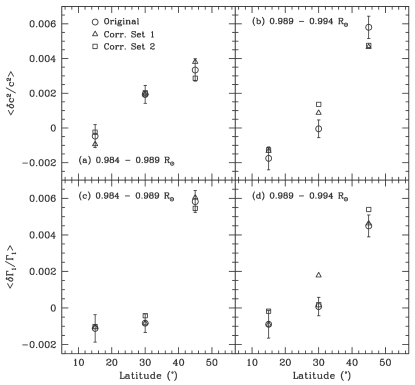
Figure 10: A comparison of the results obtained from the year 2003 (CR 2009) data and the data corrected for possible projection effects. Corr. Set 1 refers to corrections using equatorial data from 1996 and Corr. Set 2 are corrected using 1998 data. The error bars represent the $1\sigma$ statistical errors for the original data set. The errors for the corrected sets are roughly a factor of 1.4 larger.

Since we find fairly substantial latitudinal effects, it is important to look at possible systematic errors in the results, particularly those due to errors in frequencies of higher-latitude regions caused by projection effects. Although a comparison between Fig. 1 and Fig. 2 suggests that it is unlikely that the latitudinal differences we see are a result of projection effects, nonetheless we need to test this. To do so, we have subtracted the frequency differences shown in Fig. 2 from the frequency differences that we inverted. We then inverted these “corrected” sets of frequency differences. We average the results within the same radius ranges as the results in Fig. 9. The comparison for one epoch is shown in Fig. 10. In the inner radius range, the results of the corrected and uncorrected sets are very similar, all three sets being within $1\sigma$ of each other, where the standard deviations refer to those of the original set. (The errors in the “corrected” data sets are larger since the correction involved subtracting out fitted frequencies which themselves have errors.) The results for the outer radius range show greater differences. The differences are more than $1\sigma$ of the original results, but if the errors in the corrected set are considered, the results are within $1.5\sigma$. Because of this small difference, we are comfortable with the results of the original data, and we did not try to correct all of the data sets. Our decision is also supported by the fact that the results for the two corrected sets do not always lie on the same side of the original result, so they do not appear to be systematic. We conclude that Fig. 9 does represent the difference in structure between the higher latitudes and the equator.

The latitudinal variation of sound speed is even seen for the low-activity epochs, as was seen in the global-mode work of Antia et al. (2001). This may seem surprising if one assumes that the asphericity is completely a result of the magnetic field distribution. However, the latitudinal structure difference can depend on other factors. A latitudinal temperature difference is expected even in the absence of magnetic fields because of solar differential rotation which can produce a relatively cool equator and warmer poles (Thompson et al. 2003). Such a temperature differential in the outer layers translates into a difference in sound speed and $\Gamma_{1}$. Numerical simulations also show latitudinal temperature variations (Brun & Toomre 2002; Brun et al. 2004, Miesch et al. 2006, etc.), however, none of the simulations go to shallow enough layers to make a direct comparison with our results. It should be noted, however, that the simulations do not completely agree with the global-mode results. The global-mode results show a cool equator and warmer higher latitude region, while the outer layers of the simulations show a warmer equator and pole with cooler regions in between. The deeper layers in the simulations do show a cooler equator and warmer higher latitudes.

4.4.2 Changes with time

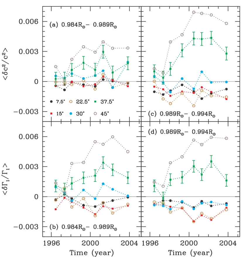
Figure 11: The averaged sound-speed and $\Gamma_{1}$ differences plotted as a function of time. Error-bars are only plotted on one set for the sake of clarity.

In order to look in detail at the time dependence of the latitudinal distribution of structure, we plot the averaged results as a function of time for different latitudes. The results are shown in Fig. 11. This figure makes it clear that the differences in structure between the highest latitudes and the equator show the greatest changes with time. This is not surprising, since the difference in magnetic field between the equator and the highest latitudes has been steadily increasing over the course of the cycle. This can be seen from the underlying color image in Fig. 8. The changes are generally larger over the outer radius range than the inner one. This is particularly true for the sound speed differences. Again, for $\Gamma_{1}$ we can see the difference in behavior below the latitude of $30^{\circ}$ and above it, with $\delta\Gamma_{1}/\Gamma_{1}$ being consistently negative for lower latitudes and positive for higher ones. This a reflection of the fact that latitudes below about $30^{\circ}$ have larger values of the MAI than the equator, while latitudes above $30^{\circ}$ have smaller values.

At lower latitudes, the sound speed differences show much smaller changes with time, though again the changes are larger in the outer radius range. $\Gamma_{1}$ shows a similar variation. It could be asked why the lower-latitude regions shows such a small change with time, when they are where the greatest concentration of magnetic fields lie. There are two possible reasons for this. The first is the rather poor latitudinal resolution of this work: the equatorial region spans a latitude range of $\pm 7.5^{\circ}$, similarly the zone centered at $7.5^{\circ}$ spans the region from the equator to $15^{\circ}$, the $15^{\circ}$ strip is from $7.5^{\circ}$ to $22.5^{\circ}$, etc. As a result, even if there are large changes at $15^{\circ}$ with respect to the equator, the poor resolution will reduce the apparent changes. Also, because of the large latitudinal range covered by the equatorial strip, substantial magnetic activity changes take place within it. Since all of our work is differential, these change are subtracted from those at other latitudes. Since the activity change in the lower latitudes has the same sign as the equator, the change in the differences between these regions and the equator is smaller. For the higher latitudes, on the other hand, any changes in structure with respect to the equator are amplified, since the magnetic field strength changes in the opposite direction.

4.4.3 Dependence on activity

Previous work by Basu et al. (2004) has shown that the sound-speed and $\Gamma_{1}$ differences between two regions increase if the difference of the MAI’s of the two regions increase. Since the MAI differences between the equator and the other latitudes change with time, we have investigated the correlations between MAI difference and the sound-speed and $\Gamma_{1}$ differences. We find that the linear correlation coefficient between the $\Gamma_{1}$ differences and the MAI differences for the 0.989–0.994$R_{\odot}$ radius range is only $-0.30$ when all data sets are used. However, the correlation rises to $-0.56$ if only sets with $|\delta{\rm MAI}|>5$ G are included. For sound speed, the correlation coefficients are smaller ($-0.27$ and $-0.46$ respectively). This small correlation is in seeming contradiction to the results of Basu et al. (2004), but not if we take into account the fact that in that paper we were dealing with MAI differences that were much larger (up to a factor of 16) than those in this work, and Basu et al (2004) had seen that the sound-speed and $\Gamma_{1}$ differences do not change much for $|\delta{\rm MAI}|$ less than about 30 G, and we are dealing with much smaller differences here.

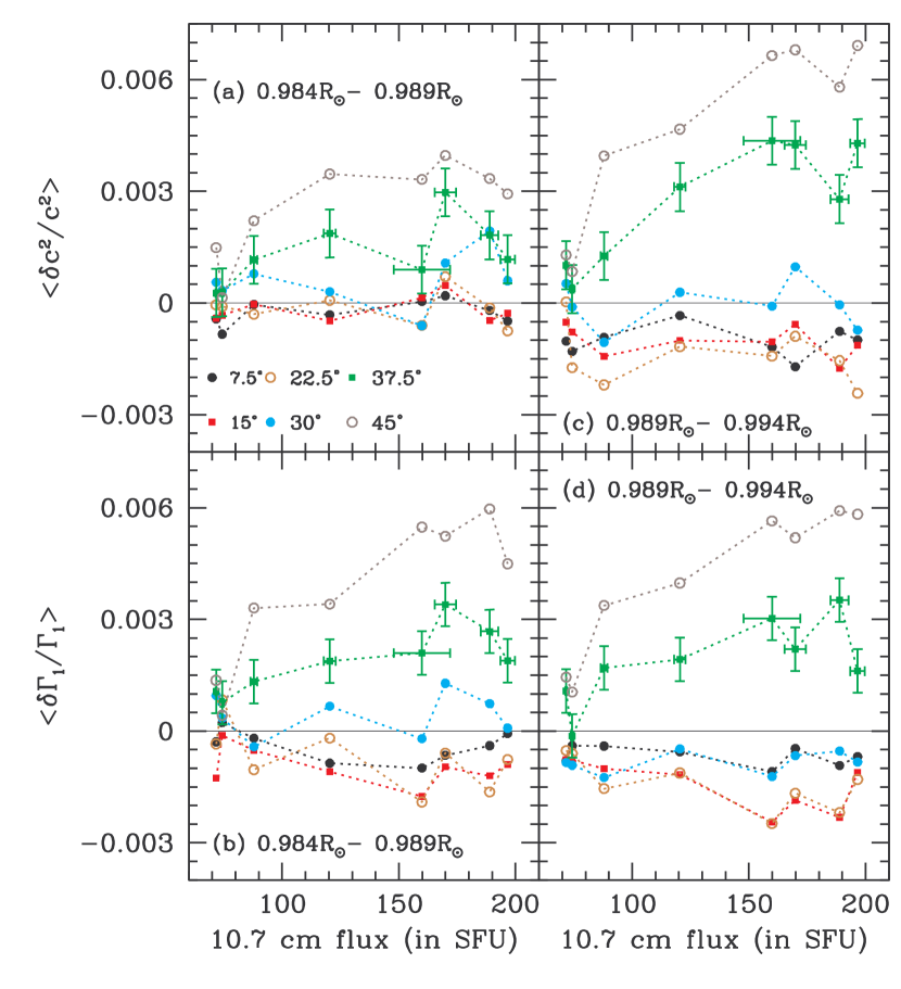
Figure 12: Same as Fig. 11, but plotted as a function of the 10.7 cm flux, a measure of global solar activity. The flux is in solar flux units, $10^{-22}$ J s^-1 m^-2 Hz^-1.

In order to study the dependence of the results on the level of global solar activity, we have plotted them as a function of the 10.7 cm radio flux. The results are shown in Fig. 12. We find as before that different latitudes show different trends.

We find that the differences between the different latitudes and the equator change with activity, particularly at the highest latitudes studied, where both $c^{2}$ and $\Gamma_{1}$ increase with activity. There seems to be a saturation of the increase at very high activity levels. This effect was also seen when we studied sound-speed differences between active and quiet regions (Basu et al. 2004). They found that the differences became nearly constant above a certain level of magnetic field strength. During the late part of the solar cycle covered by CR 1988 and CR 2009 (2002 and 2003), the average magnetic field at the equator is significantly larger than that at higher latitudes; that would also contribute to some of the observed differences. At lower latitudes, sound speed and $\Gamma_{1}$ appear to decrease with increased activity, but the results are not statistically very significant.

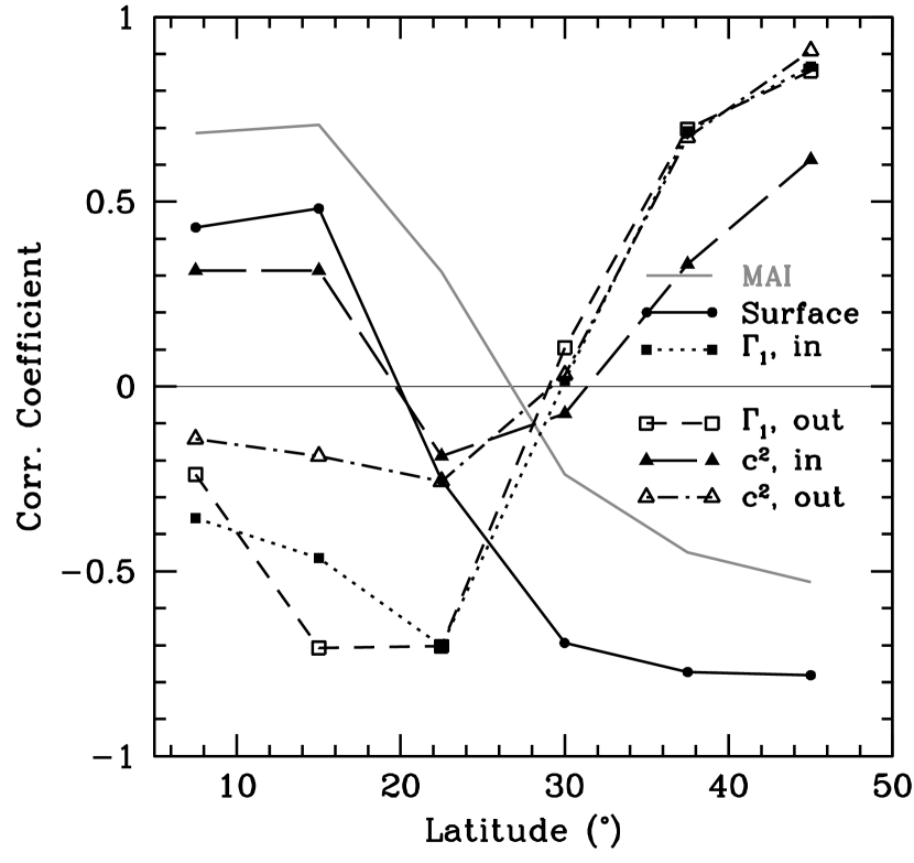
Figure 13: The correlation coefficient between different quantities and the 10.7 cm radio flux plotted as a function of latitude. The gray line shows the correlation of the 10.7 cm flux with the MAI difference between a given latitude and the equator. $\Gamma_{1}$ refers to the relative differences of $\Gamma_{1}$ between the higher latitudes and the equator, while $c^{2}$ denote the relative differences of $c^{2}$. The terms ‘in’ and ‘out’ refer to the inner and outer radius ranges, i.e., $0.984$–$0.989R_{\odot}$ and $0.989$–$0.994R_{\odot}$ respectively.

We quantify the change of $\delta c^{2}/c^{2}$ and $\delta\Gamma_{1}/\Gamma_{1}$ with the 10.7 cm flux by calculating the linear correlation coefficient. The correlation of the surface term, and $c^{2}$ and $\Gamma_{1}$ differences at each latitude with the 10.7 cm flux is shown in Fig. 13. We can see a positive correlation at high latitudes and a largely negative correlation at lower latitudes. We find that the change with solar activity is stronger for the high latitude regions than at low latitude regions, and the correlation with the 10.7 cm flux is stronger for $\Gamma_{1}$ than for $c^{2}$, and the outer-radius range (0.989–0.994$R_{\odot}$) shows a more pronounced change than the inner radius range (0.984–0.989$R_{\odot}$). We find that above $30^{\circ}$, the $\Gamma_{1}$ variation has an average correlation coefficient of $0.78$, while below $30^{\circ}$ it is $-0.5$. At $30^{\circ}$, the results show no correlation with activity at all. The correlation for $c^{2}$ differences is much weaker: for latitudes greater than $30^{\circ}$ it is 0.47 and 0.79 for the inner and outer radius ranges respectively. The lower-latitude range shows correlations only of 0.14 and $-0.19$, which are probably not statistically significant. The difference in behavior between the low and high latitudes can perhaps be attributed to the different contributions of the fields near the equator to the differences. The correlation with MAI difference also changes sign around the same latitude $30^{\circ}$. This could be because of the progression of activity toward lower latitudes with the cycle. As the activity shifts towards the equator towards the end of the solar cycle, the MAI difference between high latitudes and the equator changes sign.

4.5 Absolute time differences

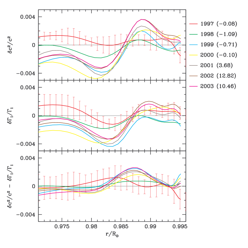
Figure 14: The sound speed and $\Gamma_{1}$ differences at the solar equator. The different lines show the differences between different epochs and CR 1910 plotted as a function of depth. Only the RLS results are shown; the SOLA results are similar. Error bars are shown for only one comparison year (1997) for the sake of clarity. The differences are in the sense (Later epoch $-$ 1996). The numbers in brackets denote the MAI differences (in Gauss) at the equator between the later epochs and 1996.

We have so far focused on the latitudinal distributions of $c^{2}$ and $\Gamma_{1}$ during each of the several Carrington rotations analyzed. The use of contemporaneous data minimizes systematic frequency errors caused by year-to-year variations of the MDI instrument, such as plate scale. If we disregard this potential problem, we can estimate the real change in $c^{2}$ and $\Gamma_{1}$ in the Sun as a function of time, and not just the change between different latitudes and the equator. Figure 14 shows how the sound speed and $\Gamma_{1}$ profiles change with time at the equator. We can see that there are changes that are statistically significant when the MAI differences between the equator at various epochs are not too small.

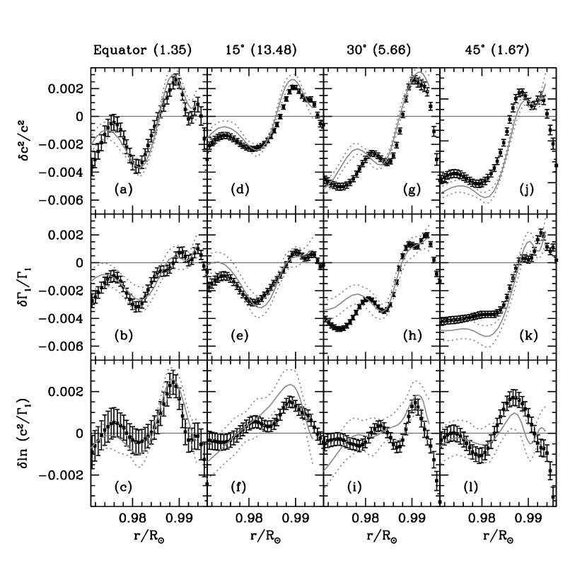
Figure 15: The sound-speed, $\Gamma_{1}$ and $c^{2}/\Gamma_{1}$ differences between the high and low activity sets at different latitudes. The latitudes are marked at the top with the MAI difference in units of Gauss given in brackets. The differences are in the sense (High Activity $-$ Low Activity). The black points are SOLA results, the error bars representing 1$\sigma$ errors, and the gray continuous lines are RLS results with the gray dotted lines showing the 1$\sigma$ error limits.

Since the errors in the results shown in Fig. 14 are large, it is difficult to judge their significance. In order to improve the signal-to-noise level of the results, we averaged the power spectra for the three sets with lowest activity (CR 1910, 1922 and 1932 in years 1996, 1997, and 1998 respectively) to produce an average power spectrum for low activity times We did the same for the three highest activity sets (CR 1964, 1975 and 1988 in years 2000, 2001, and 2002). These two average spectra were fitted in the same manner as the other data sets. We then inverted the frequency differences between the high- and low-activity sets at different latitudes. The errors in the inversion results should improve by more than the factor of $\sqrt{3}$ in the fitted frequencies themselves, because the improved signal-to-noise ratio permits us to fit many more modes. The sound-speed and $\Gamma_{1}$ differences between the high- and low-activity sets are shown in Fig. 15. We note that the fitting improvements have also translated into better agreement between the RLS and SOLA inversion results. The first thing to note from Fig. 15 is that the differences in $c^{2}$ and $\Gamma_{1}$ between times of low and high activity are statistically significant over the whole depth range. The difference for perturbations in $c^{2}/\Gamma_{1}$ is significant over a narrower range, being essentially zero below about $0.98R_{\odot}$. The general shape of the differences at the equator is similar to that seen in Fig. 14. For these sets we find that the sound speed and adiabatic index in the near-surface regions for the radius range $0.986<r/R_{\odot}<0.995$ was higher at all latitudes when the Sun was active. This is the opposite of what we found when studying the difference between active and quiet regions (Basu et al. 2004), where we found that active regions had lower sound speeds in the near surface layers than the quiet regions for $r/R_{\odot}>0.99$. The results are however consistent for $r/R_{\odot}>0.995$. There are several possible explanations for this phenomenon. It could be that the expected average negative sound-speed and $\Gamma_{1}$ differentials lie in a shallower radius range because the MAI differences that we are dealing with in this work are smaller. The results could also mean that the frequency shifts for entire latitude zones of an active Sun do not appear to be just the average of those for the active regions. It is of course possible that some of this difference is due to the fact that we are not including the direct effects of the magnetic fields in inversions. It is also possible that the results are affected by time-dependent systematic effects, such as changes in the MDI focus.

4.6 Differences between the northern and southern hemispheres

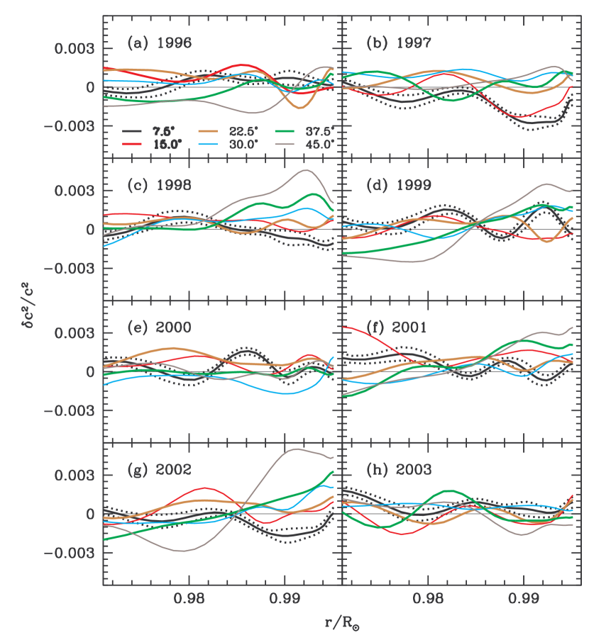
Figure 16: The difference in sound speed between the northern and southern hemispheres of the Sun as a function of depth. $1\sigma$ error limits are shown as dotted lines. Errors are shown only for 7.5^∘ for the sake of clarity. Only RLS results are shown.

In the previous sections we examined only averaged results for symmetric latitude zones in the northern and southern hemispheres. One of the advantages of ring-diagram over global-mode analysis is that it permits us to look for north-south asymmetries by inverting the frequency differences between corresponding latitude zones in the two hemispheres. Figure 16 shows the difference between the northern and southern hemisphere sound speeds. The results for $\Gamma_{1}$, which are not shown, are quite similar. There is no discernible pattern; there are clearly significant hemispheric differences at some times for some latitudes, but no consistent trends. We frequently find large asymmetries at the higher latitudes ($37.5^{\circ}$ and $45^{\circ}$), but the differences are not always statistically significant.

One of the more interesting features is the north-south asymmetry at $\pm 45^{\circ}$ latitude for data from 1999 and 2002 (see panels d and g of Fig. 16). There is a very large difference between the northern and the southern hemisphere in the deeper layers. We cannot be certain about the reality of that feature at $45^{\circ}.$ Haber et al. (2002) found submerged counter-flowing meridional flow cells at these depths in the northern hemisphere only in 1999 and 2001. It has been argued that the the countercell feature in the meridional flow can be caused by data errors (see e.g., Bogart & Basu 2004); if so, this feature in the sound-speed differences could have the same origin. We do not see any similar feature in the 2001 data, however. Haber et al. (2002) did not analyze 2002 data, so the present result cannot yet be directly compared with meridional flow asymmetries.

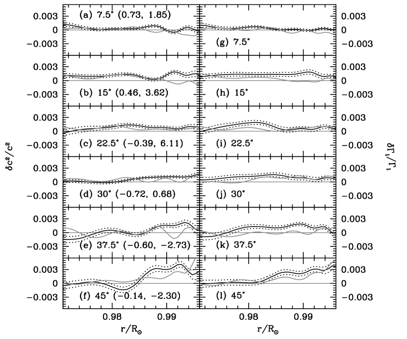
Figure 17: The north-south differences in $c^{2}$ (panels a–f) and $\Gamma_{1}$ (panels g–l) for the averaged high activity set (black) and the averaged low activity set (gray). Differences are in the sense (North $-$ South). The bracketed pair of numbers in panels a–f are MAI differences for that latitude for the low- and high-activity sets respectively. Error (as dotted lines) are shown for only the high-activity set for clarity. Only SOLA results are shown; RLS results are very similar.

Given that the north-south asymmetries for individual epochs are small, we again use the low-activity and high-activity average spectra of § 4.5 to improve the signal-to-noise ratio. We examine the difference signals separately for the low-activity and high-activity data. The results for both $c^{2}$ and $\Gamma_{1}$ differences between the northern and the southern hemispheres are shown in Fig. 17. It is quite clear that there is little evidence of asymmetry at low latitudes, as the differences are generally at the 2–3$\sigma$ level. At higher latitudes ($>30^{\circ}$), the difference between the hemispheres is clearer, particularly for the high-activity set. In general, the asymmetry appears larger at the higher activity epoch. It thus appears that there was some significant difference in structure at high latitudes during the active phase of cycle 23. This by itself is not surprising: many activity-related observations show north-south asymmetry; e.g., de Toma et al. (2000) found that at the end of cycle 22 and onset of cycle 23, Kitt Peak magnetograms show a north-south asymmetry. North-south differences have also been found in the distribution of solar flares (e.g., Bai 1990) and magnetic filaments (e.g., Duchlev & Dermendjiev 1996), and in the photospheric magnetic flux (e.g., Howard 1974; Knaack et al. 2004). The fact that the low-activity set has a lower north-south difference than the high-activity one is consistent with the fact that the MAI differences for the low-activity sets are smaller than those of the high-activity ones. However, for any given set, the differences are not what we expect from the MAI differences. We would have expected, for example, a larger difference at 22.5^∘ for the high-activity set than for the 45^∘ set, but we see the opposite. These results could again be an indication that averaging of non-contemporaneous ring-diagram spectra may not be the correct thing to do because of possible time-dependent systematic observational effects.

5 Conclusions

We have analyzed data from eight full Carrington rotations to determine the latitudinal distribution of the axisymmetric components of sound speed and $\Gamma_{1}$, and to determine whether those distributions change with time and magnetic activity level. Ring-diagram analysis allows us to determine frequencies of high-degree modes, permitting us to determine solar structure in the near-surface layers, where most solar-cycle related changes are believed to occur. Our results are valid in the radius range $0.975$–$0.996R_{\odot}$ and most reliable in the range $0.985$–$0.995R_{\odot}$. We have studied latitudes up to $\pm 45^{\circ}$.

For all epochs studied, we find significant frequency differences between the equator and the higher latitudes. These differences cannot be explained as being caused by projection effects alone; most of the differences are believed to reflect physical causes. Assuming that the frequency differences are caused by differences in structure alone, we have inverted them to determine the sound speed and the adiabatic index differences between the equator and higher latitudes. We find significant differences in structure between the equator and the higher latitudes for all epochs. The differences are largest for latitudes $>30^{\circ}$. These regions tend to have higher sound speed and $\Gamma_{1}$ than the equator. The differences in $\Gamma_{1}$ between the equator and higher latitudes imply temperature changes in these regions. Using global modes, Antia et al. (2001) also found a region of positive sound speed difference around a latitude of $60^{\circ}$. Although the magnitude of the difference is much smaller in deeper layers, of the order of $10^{-4}$, the qualitative behavior is similar. We expect the relative magnitude of the effect to increase in the near surface layers, as the global analysis suggests that most of the temporal variations in the solar oscillation frequencies arise from the surface layers. Because of the low pressure near the surface, magnetic fields are expected to be more effective in modifying the structure.

We find that the surface term from the inversions changes with time. The surface term is reasonably correlated with the difference between the magnetic activity index of the higher latitude regions and the equator. The correlation improves if only $|\delta{\rm MAI}|>5$ G regions are considered. The surface term is also correlated with the 10.7 cm flux, though the correlation is strongly dependent on the latitude. The latitudinal dependence of the correlation coefficient can be explained by changes in the latitudinal distribution of the magnetic field as solar activity changes.

The asphericity of the Sun changes with time, with the difference between the higher latitudes and the Equator increasing with increasing levels of activity. The differences can be explained by the change in the magnetic field distribution on the Sun as the activity level increases. The change with time and activity is in opposite directions for latitudes above and below $30^{\circ}$. This is consistent with the evolution of the magnetic field distribution. As with the surface term, the differences are correlated both with local and global magnetic field indices. The magnitude of changes between the active and quiet periods seen in this study is about a factor of 3–10 less than what was observed between individual active and quiet regions (Basu et al. 2004). This is expected, as the average magnetic field strength over a whole latitude band is much smaller than that in active regions alone. Although it is difficult to separate the effects of magnetic field and structural variations, one may expect the magnetic field to play a significant role near the surface. The ratio of magnetic to gas pressure is expected to be comparable, to order of magnitude, to the variations found in sound speed. At $r=0.99R_{\odot}$ a variation of $10^{-3}$ may correspond to a magnetic field of 4000 G, which is considerably larger than the typical magnetic field observed at the surface.

We have also looked at temporal variations of structure by inverting the frequency differences between times when the Sun was active (2000–2002) and when it was relatively quiet (1996–1998). Assuming that there are no time-dependent systematic errors in the data, these differences were inverted to look at how the structure of the outer layers of the Sun differed during the two epochs. We find that there are significant differences in the near-surface structure of the Sun during quiet and active periods. These results, however, may be affected by systematic observational variations. It is also possible that the results are systematically biased in some subtle way by the different projection effects involved in tracking or not tracking the data.

We have also studied the north-south asymmetries in the structure of the outer layers of the Sun. We find that when the Sun was active during cycle 23, the sound speed in the northern hemisphere was higher than that in the southern hemisphere, at least at high latitudes. Somewhat similar behavior is seen for $\Gamma_{1}$. This can be explained by differing amounts of asymmetry in the magnetic fields of the northern and southern hemispheres when the Sun was quiet and when the Sun was active.

Table 1: Data sets analyzed

Carrington	Dates	10.7 cm Flux
Rotation		(SFU)1
1910	1996:06:01 – 1996:06:28	$\phantom{0}71.7\pm 0.3$
1922	1997:04:24 – 1997:05:22	$\phantom{0}74.3\pm 0.6$
1932	1998:01:22 – 1998:02:18	$\phantom{0}87.9\pm 1.5$
1948	1999:04:04 – 1999:05:01	$120.4\pm 2.5$
1964	2000:06:13 – 2000:07:10	$188.9\pm 3.8$
1975	2001:04:09 – 2001:05:06	$169.9\pm 4.6$
1988	2002:03:30 – 2002:04:26	$196.6\pm 3.1$
2009	2003:10:18 – 2003:11:15	$159.9\pm 12.1$

References

- Antia & Basu (1994) Antia, H. M., & Basu, S. 1994, A&AS, 107, 421
- Antia et al. (2001) Antia, H. M., Basu, S., Hill, F., Howe, R., Komm, R. W., & Schou, J. 2001, MNRAS, 327, 1029
- Antia et al. (2003) Antia, H. M., Chitre, S. M., & Thompson, M. J. 2003, A&A, 399, 329
- Bai (1990) Bai, T. 1990, ApJ, 364, L17
- Balmforth (1992) Balmforth, N. J. 1992, MNRAS, 255, 632
- Basu (2002) Basu, S. 2002, in From Solar Min to Max: Half a Solar Cycle with SOHO, Proc. SOHO 11 Symposium, ed., A. Wilson, ESA SP-508, 7
- Basu & Antia (1999) Basu, S., & Antia, H. M. 1999, ApJ, 525, 517
- Basu & Antia (2000) Basu, S., & Antia, H. M. 2000, ApJ, 541, 442
- Basu & Antia (2002) Basu, S., & Antia, H. M. 2002, in From Solar Min to Max: Half a Solar Cycle with SOHO, Proc. SOHO 11 Symposium, ed., A. Wilson, ESA SP-508, 59
- Basu & Antia (2003) Basu, S., & Antia, H. M. 2003, ApJ, 585, 553
- Basu & Mandel (2004) Basu, S., & Mandel, A. 2004, ApJ, 617, L155
- Basu & Thompson (1996) Basu, S., & Thompson, M. J. 1996, A&A, 305, 631
- Basu, Antia & Tripathy (1999) Basu, S., Antia, H. M., & Tripathy, S. C. 1999, ApJ, 512, 458
- Basu et al. (2004) Basu, S., Antia, H. M., & Bogart, R. S. 2004, ApJ, 610, 1157
- Bogart & Basu (2004) Bogart, R.S., & Basu, S. 2004, in Proc: SOHO 14 / GONG 2004 Workshop “Helio- and Asteroseismology: Towards a Golden Future”, ESA SP-559, 329
- Brun & Toomre (2002) Brun, A.S., Toomre, J. 2002, ApJ, 570, 865
- Brun et al. (2004) Brun, A.S., Miesch, M., Toomre, J. 2004, ApJ, 614, 1073
- Chou & Serebryanskiy (2005) Chou, D.-Y., & Serebryanskiy, A. 2005, ApJ, 624, 420
- (19) Cox, A. N., & Kidman, R. B. 1984, in Theoretical problems in stellar stability and oscillations (Liège: Institut d’Astrophysique), 259
- Dappen et al. (1991) Däppen, W., Gough, D. O., Kosovichev, A. G., & Thompson, M. J. 1991, in Challenges to Theories of the Structure of Moderate-Mass Stars, eds., D. Gough & T. Toomre, Lecture notes in Physics, 388, 111
- de Toma et al. (2000) de Toma, G., White, O. R., & Harvey, K. L. 2000, ApJ, 529, 1101
- Duchlev & Dermendjiev (1996) Duchlev, P. I., & Dermendjiev, V. N. 1996, Sol. Phys., 168, 205
- Duvall et al. (1993) Duvall, T. L., Jr., Jefferies, S. M., Harvey, J. W., & Pomerantz, M. A. 1993, Nature, 362, 430
- Dziembowski et al. (1990) Dziembowski, W. A., Pamyatnykh, A. A., & Sienkiewicz, R. 1990, MNRAS, 244, 542
- Dziembowski et al. (1994) Dziembowski, W. A., Goode, P. R., Pamyatnykh, A. A., & Sienkiewicz, R. 1994, ApJ, 432, 417
- Eff-Darwich et al. (2002) Eff-Darwich, A., Korzennik, S. G., Jiménez-Reyes, S. J., & Pérez Hernández, F. 2002, ApJ, 580, 574
- Gough et al. (1996) Gough, D. O., Kosovichev, A. G., Toomre, J. et al., 1996, Science, 272, 1296
- Haber et al. (2002) Haber, D. A., Hindman, B. W., Toomre, J., Bogart, R. S., Larsen. R. M., & Hill, F. 2002, ApJ, 570, 855
- Hill (1988) Hill, F. 1988, ApJ, 333, 996
- Hindman et al. (2000) Hindman, B. W., Haber, D., Toomre, J., & Bogart, R. 2000, Sol. Phys., 192, 363
- Howard (1974) Howard, R. 1974, Sol. Phys., 38, 59
- Howe et al. (2000) Howe R., Christensen-Dalsgaard J., Hill F., Komm R. W., Larsen R. M., Schou J., Thompson M. J., & Toomre J. 2000, ApJ 533, L163
- Howe et al. (2004a) Howe, R., Komm, R. W., Hill, F., Christensen-Dalsgaard, J., Haber, D. A., Schou, J., & Thompson, M. J. 2004a, in Proc. SOHO 14/ GONG 2004 11 “Helio- and Asteroseismology: Towards a Golden Future” ESA SP-559, 472
- Howe et al. (2004b) Howe, R., Komm, R. W., Hill, F., Haber, D. A., & Hindman, B. W. 2004b, ApJ 608, 562
- Knaack et al. (2004) Knaack, R., Stenflo, J. O., & Berdyugina, S. V. 2004, A&A, 418, L17
- Korzennik et al. (2004) Korzennik, S. G., Rabello-Soares, M. C., & Schou, J. 2004, ApJ, 602, 481
- Kosovichev et al. (2000) Kosovichev, A. G., Duvall, T. L., Jr., & Scherrer, P. H. 2000, Solar Phys., 192, 159
- Kosovichev et al. (2001) Kosovichev, A. G., Duvall, T. L., Jr., Birch, A. C., Gizon, L., Scherrer, P. H., & Zhao, J. 2001, in Helio- and Asteroseismology at the Dawn of the Millennium, Proc. SOHO 10/GONG 2000 Workshop, ed., A. Wilson, ESA SP-464, 701
- Miesch et al. (2006) Miesch, M.S., Brun, A.S., Toomre, J. 2006, ApJ, 641, 618
- Patrón et al. (1997) Patrón, J., et al. 1997, ApJ, 485, 869
- Pijpers & Thompson (1992) Pijpers, F. P., & Thompson, M. J. 1992, A&A, 262, L33
- Pijpers & Thompson (1994) Pijpers, F. P., & Thompson, M. J. 1994, A&A, 281, 231
- Rabello-Soares et al. (1999) Rabello-Soares, M. C., Basu, S., & Christensen-Dalsgaard, J. 1999, MNRAS, 309, 35
- Rajaguru et al. (2001) Rajaguru, S. P., Basu, S., & Antia, H. M. 2001, ApJ, 563, 410
- Schou (1999) Schou, J., 1999, ApJ, 523, L181
- Schou et al. (1998) Schou, J., Antia, H. M., Basu, S. et al., 1998, ApJ, 505, 390
- Sekii (1997) Sekii, T. 1997, in Proc. IAU Symp. 181: Sounding Solar and Stellar Interiors, eds. J Provost, F.-X. Schmider, Dordrecht: Kluwer, 189
- Thompson et al. (1996) Thompson, M. J., Toomre, J., Anderson, E. R. et al., 1996, Science, 272, 1300
- Thompson et al. (2003) Thompson, M. J., Christensen-Dalsgaard, J., Miesch, M.S., Toomre, J. 2003, ARA&A, 41, 599
- Verner et al. (2006) Verner, G.A., Chaplin, W.J., Elsworth, Y. 2006, ApJ, 640, L95