Prospects for direct detection of circular polarization of gravitational-wave background

Abstract

We discussed prospects for directly detecting circular polarization signal of gravitational wave background. We found it is generally difficult to probe the monopole mode of the signal due to broad directivity of gravitational wave detectors. But the dipole $(l=1)$ and octupole $(l=3)$ modes of the signal can be measured in a simple manner by combining outputs of two unaligned detectors, and we can dig them deeply under confusion and detector noises. Around $f\sim 0.1$mHz LISA will provide ideal data streams to detect these anisotropic components whose magnitudes are as small as $\sim 1$ percent of the detector noise level in terms of the non-dimensional energy density $\Omega_{GW}(f)$.

I introduction

As gravitational interaction is very weak, significant efforts have been made to detect gravitational waves. But, on the other hand, we will be able to get rich information of the universe by observing gravitational waves that directly propagate to us with almost no absorption. Various astrophysical and cosmological models predict existence of stochastic gravitational wave background, and it is an interesting target for gravitational wave astronomy Allen:1996vm . For its observational prospects, we need to understand how we characterize the background and what aspects we can uncover with current and future observational facilities.

One of such aspects is circular polarization that describes whether the background has asymmetry with respect to magnitudes of right- and left-handed waves. Circular polarization of gravitational wave background might be generated by helical turbulent motions (see e.g. Kahniashvili:2005qi and references therein). Inflation scenario predicts gravitational wave background from quantum fluctuations during acceleration phase in the early universe, but asymmetry of left and right-handed waves can be produced with the gravitational Chern-Simon term that might be derived from string theory and might be related to creation of baryon number (see e.g. Lyth:2005jf and references therein). Primordial gravitational wave background, including information of its circular polarization Lue:1998mq , can be indirectly studied with CMB measurement Seljak:1996gy at very low frequency regime $f\sim 10^{-17}$Hz that is largely different from the regime directly accessible with gravitational wave detectors studied in this Letter. Gravitational wave background from Galactic binaries can be polarized, if orientation of their angular momentum have coherent distribution, such as, correlation with Galactic structure. While observational samples of local Galactic binaries do not favor such correlation inc , this will also be an interesting target that can be directly studied with LISA.

It is well known that observation of gravitational wave is intrinsically sensitive to its polarization state Thorne_K:1987 . This is because we measure spatial expansion and contraction due to the wave, and polarization determines the direction of the oscillation perpendicular to its propagation direction. Another important nature of the observation is that we have to simultaneously deal with waves basically coming from all the directions, in contrast to observations with typical electromagnetic wave telescopes that have sharp directivity. Therefore, polarization information and directional information couple strongly in observational analysis of gravitational wave background. In general, orientation of a gravitational wave detector changes with time, and induced modulation of data stream is useful to probe the polarization and directional information. For ground based detectors, such as, LIGO, this is due to the daily rotation of the Earth Allen:1996gp . For a space mission like LISA, this change is determined by its orbital choice lisa ; Cornish:2001qi . In addition, we can also expect that several independent data streams of gravitational waves will be taken at the same time Cutler:1997ta ; Prince:2002hp . In this Letter, in view of these observational characters, we study how well we can extract information of circular polarization of the background in a model independent manner about its origin.

II formulation

The standard plane wave expansion of metric perturbation by gravitational waves is given as

$$h_{ab}(t,{\mbox{\boldmath${x}$}})=\sum_{P=+,\times}\int^{\infty}_{-\infty}df\int_{S^{2}}d\mbox{\boldmath${n}$}h_{P}(f,\mbox{\boldmath${n}$})e^{2\pi if(t-\mbox{\boldmath${n}$}\cdot{\mbox{\boldmath${x}$}})}{\mbox{\boldmath${e}$}}^{P}_{ab}(\mbox{\boldmath${n}$}),$$ (1)

where $S^{2}$ is the unit sphere for the angular integral, the unite vector $\mbox{\boldmath${n}$}=(\sin\theta\cos\phi,\sin\theta\sin\phi,\cos\theta)$ is propagation direction, and ${\mbox{\boldmath${e}$}}^{+}_{ab}$ and ${\mbox{\boldmath${e}$}}^{\times}_{ab}$ are the basis for the transverse-traceless tensor. We fix them as ${\mbox{\boldmath${e}$}}^{+}_{ab}={\hat{\mbox{\boldmath${e}$}}}_{\theta}\otimes{\hat{\mbox{\boldmath${e}$}}}_{\theta}-{\hat{\mbox{\boldmath${e}$}}}_{\phi}\otimes{\hat{\mbox{\boldmath${e}$}}}_{\phi}$ and ${\mbox{\boldmath${e}$}}^{\times}_{ab}={\hat{\mbox{\boldmath${e}$}}}_{\theta}\otimes{\hat{\mbox{\boldmath${e}$}}}_{\phi}+{\hat{\mbox{\boldmath${e}$}}}_{\phi}\otimes{\hat{\mbox{\boldmath${e}$}}}_{\theta}$ where ${\hat{\mbox{\boldmath${e}$}}}_{\theta}$ and ${\hat{\mbox{\boldmath${e}$}}}_{\phi}$ are two unit vectors with a fixed spherical coordinate system. As the metric perturbation $h_{ab}(t,{\mbox{\boldmath${x}$}})$ is real, we have a relation for complex conjugate; $h_{P}(-f,\mbox{\boldmath${n}$})=h_{P}(f,\mbox{\boldmath${n}$})^{*}$. When we replace the direction $\mbox{\boldmath${n}$}\to-\mbox{\boldmath${n}$}$, the matrices have correspondences ${\mbox{\boldmath${e}$}}^{+}_{ab}\to{\mbox{\boldmath${e}$}}^{+}_{ab}$ (even parity) and ${\mbox{\boldmath${e}$}}^{\times}_{ab}\to-{\mbox{\boldmath${e}$}}^{\times}_{ab}$ (odd parity).

To begin with, we study gravitational wave modes at a frequency $f$. Here, we omit explicit frequency dependence for notational simplicity, unless we need to keep it. The covariance matrix $\left(\begin{array}[]{@{\,}cc@{\,}}\left\langle h_{+}(\mbox{\boldmath${n}$})h_{+}^{*}(\mbox{\boldmath${n}$}^{\prime})\right\rangle&\left\langle h_{+}(\mbox{\boldmath${n}$})h_{\times}^{*}(\mbox{\boldmath${n}$}^{\prime})\right\rangle\\ \left\langle h_{+}^{*}(\mbox{\boldmath${n}$})h_{\times}(\mbox{\boldmath${n}$}^{\prime})\right\rangle&\left\langle h_{\times}(\mbox{\boldmath${n}$})h_{\times}^{*}(\mbox{\boldmath${n}$}^{\prime})\right\rangle\\ \end{array}\right)$ for two polarization modes $h_{+}(\mbox{\boldmath${n}$})$ and $h_{\times}(\mbox{\boldmath${n}$})$ is decomposed as

$$\frac{\delta_{drc}(\mbox{\boldmath${n}$}-\mbox{\boldmath${n}$}^{\prime})}{4\pi}\left(\begin{array}[]{@{\,}cc@{\,}}I+Q&U-iV\\ U+iV&I-Q\\ \end{array}\right),$$ (2)

where the symbol $\left\langle\dots\right\rangle$ represents to take an ensemble average for superposition of stationary incoherent waves, and $\delta_{drc}(\cdot)$ is the delta function on the unit sphere $S^{2}$. We have defined the following Stokes parameters radipro analog to electromagnetic waves as $I(\mbox{\boldmath${n}$})=\left\langle|h_{+}|^{2}+|h_{\times}|^{2}\right\rangle/2,~{}~{}Q(\mbox{\boldmath${n}$})=\left\langle|h_{+}|^{2}-|h_{\times}|^{2}\right\rangle/2,~{}~{}U(\mbox{\boldmath${n}$})=\left\langle h_{+}h_{\times}^{*}+h_{+}^{*}h_{\times}\right\rangle/2,$ and $V(\mbox{\boldmath${n}$})=i\left\langle h_{+}h_{\times}^{*}-h_{+}^{*}h_{\times}\right\rangle/2.$ The parameter $I(\mbox{\boldmath${n}$})$ represents the total intensity of the wave, while $Q(\mbox{\boldmath${n}$})$ and $U(\mbox{\boldmath${n}$})$ is related to linear polarization. The parameter $V(\mbox{\boldmath${n}$})$ is related to circular polarization, and its sign shows whether right- or left-handed waves dominate. When we rotate the basis vectors ${\hat{\mbox{\boldmath${e}$}}}_{\theta}$ and ${\hat{\mbox{\boldmath${e}$}}}_{\phi}$ around the axis ${n}$ by angle $\psi$, the parameters $I$ and $V$ are invariant (spin 0). But the parameters $Q$ and $U$ are transformed as $(Q\pm iU)^{\prime}(\mbox{\boldmath${n}$})=e^{\mp 4i\psi}(Q\pm iU)(\mbox{\boldmath${n}$}),$ and the combinations $(Q\pm iU)(\mbox{\boldmath${n}$})$ have spin $\pm 4$ radipro .

Next we discuss response of a two-arm interferometer $J$ with $90^{\circ}$ vertex angle and equal arm-length $L$. We put $\mbox{\boldmath${l}$}_{1}$ and $\mbox{\boldmath${l}$}_{2}$ as unit vectors for the directions of the arms. The beam pattern functions $F_{J}^{P}=(\mbox{\boldmath${l}$}_{1}\cdot{\mbox{\boldmath${e}$}}^{P}\cdot\mbox{\boldmath${l}$}_{1}-\mbox{\boldmath${l}$}_{2}\cdot{\mbox{\boldmath${e}$}}^{P}\cdot\mbox{\boldmath${l}$}_{2})/2$ $(P=+,\times)$ represent relative sensitivities to two linearly polarized gravitational waves ($P=+,\times$) with various directions ${n}$ Thorne_K:1987 . Note that the function $F_{J}^{+}$ has even parity and $F_{J}^{\times}$ has odd parity with respect to the direction ${n}$ (see e.g. Kudoh:2004he ).

In this Letter we mainly deal with low frequency regime with $f/f_{*}\ll 1$. Here, using the arm-length $L$, we have defined a characteristic frequency $f_{*}=1/(2\pi L)$ that corresponds to 10mHz for LISA and 1Hz for Big Bang Observer (BBO) bbo ; Seto:2005qy . LISA is formed by three spacecrafts that nearly keep a regular triangle configuration lisa . From its six one-way data streams, we can make Time-Delay-Interferometer (TDI) variables that cancel laser frequency noises. We can select three TDI variables $A$, $E$ and $T$ whose detector noises are not correlated and can be regarded as independent Prince:2002hp . At the low frequency regime the responses of the $A$ and $E$ modes can be effectively regarded as those of two-arm interferometers whose configuration are shown in figure 1 Cutler:1997ta . In this figure we put the whole system on $XY$-plane ($\theta=\pi/2$). The beam pattern functions of the $A$ mode are explicitly given as

$$F_{A}^{+}(\theta,\phi)=\frac{1}{2}(1+\cos^{2}\theta)\cos 2\phi,~{}~{}~{}F_{A}^{\times}(\theta,\phi)=-\cos\theta\sin 2\phi,$$ (3)

while those for the $E$ mode are given by replacing $\phi\to\phi-\pi/4$ in the above expressions. The beam pattern functions for the $T$ mode are quite different from the $A$ and $E$ modes, and given as $F_{T}^{P}=\sum_{i=1}^{3}(\mbox{\boldmath${m}$}_{i}\cdot{\mbox{\boldmath${e}$}}^{P}\cdot\mbox{\boldmath${m}$}_{i})(\mbox{\boldmath${m}$}_{i}\cdot\mbox{\boldmath${n}$})$ $(P=+,\times)$ where directions of three unit vectors $\mbox{\boldmath${m}$}_{i}$ are shown in figure 1 Kudoh:2004he ; Tinto:2001ii . At low frequency regime sensitivity of the $T$ mode to gravitational waves is $\sim(f/f_{*})^{-1}$ times worse than those for the $A$ and $E$ modes Prince:2002hp ; Tinto:2001ii . Therefore we put this mode aside for a while.

We can express responses of the $A$ and $E$ modes to gravitational waves from a single direction ${n}$ as $(J=A,E)$

$$r_{J}(\mbox{\boldmath${n}$})=\left(F_{J}^{+}h_{+}(\mbox{\boldmath${n}$})+F_{J}^{\times}h_{\times}(\mbox{\boldmath${n}$})\right)\left[1+i(f/f_{*})D_{J}(\mbox{\boldmath${n}$})+O(f^{2}/f_{*}^{2})\right],$$ (4)

where the second factor $\left[\dots\right]$ is corrections caused by the finiteness of the arm-length, and two real functions $D_{A}(\theta,\phi)$ and $D_{E}(\theta,\phi)$ depend on the propagation directions ${n}$ of waves (see e.g. Kudoh:2004he ). In eq.(4) we neglected overall factors that depend only on frequency $f$ and are irrelevant for our study. These formal expressions for the perturbative expansion with respect to the ratio $(f/f_{*})$ can be generally used with relevant beam pattern functions, including the case for the $T$-mode or Fabri-Perot detectors as LIGO.

The information $V$ cannot be produced from the response $r_{A}$ or $r_{E}$ alone. To get it we need independent linear combination of $h_{+}$ and $h_{\times}$. For example the term $\left\langle r_{A}(\theta,\phi)r_{A}(\theta,\phi)^{*}\right\rangle$ can be written only with $I,Q$ and $U$. We now take the low frequency limit, and keep only the leading order terms of the expansions. The cross term $\left\langle r_{A}(\mbox{\boldmath${n}$})r_{E}(\mbox{\boldmath${n}$}^{\prime})^{*}\right\rangle$ is given as

$$\left\langle r_{A}(\mbox{\boldmath${n}$})r_{E}(\mbox{\boldmath${n}$}^{\prime})^{*}\right\rangle = \frac{\delta_{drc}(\mbox{\boldmath${n}$}-\mbox{\boldmath${n}$}^{\prime})}{4\pi}{\Bigg{\{}}\frac{1}{2}\left[\left(\frac{1+\cos^{2}\theta}{2}\right)^{2}-\cos^{2}\theta\right]\sin 4\phi I(\theta,\phi)+\frac{1}{2}\left[\left(\frac{1+\cos^{2}\theta}{2}\right)^{2}+\cos^{2}\theta\right]\sin 4\phi Q(\theta,\phi)$$ (5)

$$+\left[\left(\frac{1+\cos^{2}\theta}{2}\right)\cos\theta\right]\cos 4\phi U(\theta,\phi)-i\left[\left(\frac{1+\cos^{2}\theta}{2}\right)\cos\theta\right]V(\theta,\phi){\Bigg{\}}}.$$

With the following combination

$${\rm Im}\left[\left\langle r_{A}(\mbox{\boldmath${n}$})r_{E}(\mbox{\boldmath${n}$}^{\prime})^{*}\right\rangle\right]=-\frac{\delta_{drc}(\mbox{\boldmath${n}$}-\mbox{\boldmath${n}$}^{\prime})}{4\pi}\left[\left(\frac{1+\cos^{2}\theta}{2}\right)\cos\theta\right]V(\theta,\phi)$$ (6)

we can extract the circular parameter $V$ alone. As shown in figure 1, the effective detector $E$ is obtained by rotating the detector $A$ around $Z$-axis by $\pi/4$ Cutler:1997ta . If this angle is $\delta$, there appears a factor $\sin 2\delta$ in the final expression in eq.(6). Therefore, in some sense, LISA will provide an optimal set $(A,E)$ to study the parameter $V$. In contrast, sensitivity of correlation analysis to the monopole intensity $I_{00}$ is proportional to $\cos 2\delta$, and LISA cannot probe it with the method, as is well known.

We now discuss responses of detectors to gravitational waves from all directions ${n}$. Firstly, what we can get observationally form the $A$ and $E$ modes are the following integrals $R_{A}=\int r_{A}(\mbox{\boldmath${n}$})d\mbox{\boldmath${n}$}$ and $R_{A}=\int r_{A}(\mbox{\boldmath${n}$})d\mbox{\boldmath${n}$}$. Considering the spin of quantities $I$, $Q\pm iU$ and $V$ we can expand them in terms of the spin weighted spherical harmonics ${}_{s}Y_{lm}$ as $I(\theta,\phi)=\sum I_{lm}Y_{lm}(\theta,\phi),~{}~{}~{}(Q\pm iU)(\theta,\phi)=\sum K_{\pm,lm}\cdot{}_{\pm 4}Y_{lm}(\theta,\phi),~{}~{}~{}V(\theta,\phi)=\sum V_{lm}Y_{lm}(\theta,\phi),$ where the coefficients $K_{\pm,lm}$ are defined for $l\geq 4$. With these harmonic expansions and eq.(6), the combination ${\cal C}={\rm Im}\left\langle R_{A}R_{E}^{*}\right\rangle$ is evaluated as ${\cal C}=-\frac{8}{5}\sqrt{\frac{\pi}{3}}V_{10}-\frac{2}{5}\sqrt{\frac{\pi}{7}}V_{30}.$ When we rotate two interferometers $A$ and $E$ with Euler angles $(\alpha,\beta,\gamma)$, the signal ${\cal C}$ becomes

$${\cal C}(\alpha,\beta,\gamma)=-\frac{16\pi}{15}V_{1m}Y_{1m}(\alpha,\beta)-\frac{4\pi}{35}V_{3m}Y_{3m}(\alpha,\beta).$$ (7)

This result is obtained by relating the coefficients $V_{lm}$ in original coordinate with those in rotated coordinate Allen:1996gp . LISA moves around the Sun with changing the orientation of its detector plane that is inclined to the ecliptic plane by 60 degree lisa . To describe these motions in the ecliptic coordinate, the Euler angles are given as $\alpha=2\pi(t/1{\rm yr})+\alpha_{0}$, $\beta=\pi/3$ and $\gamma=-2\pi(t/1{\rm yr})+\gamma_{0}$ with time $t$ and constants $\alpha_{0}$ and $\gamma_{0}$ Cutler:1997ta . This parameterization is also valid for BBO bbo . The parameter $\gamma$ determines the so-called cartwheel motion, but the combination ${\cal C}(\alpha,\beta,\gamma)$ does not depend on it. From eq.(7) we can understand that the observed signal ${\cal C}(\alpha,\beta,\gamma)$ with LISA is decomposed into modulation patterns with frequencies $f=0,\pm 1/3,\pm 1/2$ and $\pm 1{\rm yr^{-1}}$ from $m=0,\pm 1,\pm 2$ and $\pm 3$ modes respectively.

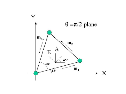
Figure 1: The effective two-arm interferometers corresponding to the TDI modes $A$ and $E$. Three spacecrafts of LISA are shown with circles that are put on the $XY$-plane ($\theta=\pi/2$). The beam pattern functions for $T$ mode are given with three unit vectors $\mbox{\boldmath${m}$}_{i}$ as $F_{T}^{P}=\sum_{i=1}^{3}(\mbox{\boldmath${m}$}_{i}\cdot{\mbox{\boldmath${e}$}}^{P}\cdot\mbox{\boldmath${m}$}_{i})(\mbox{\boldmath${m}$}_{i}\cdot\mbox{\boldmath${n}$})$ $(P=+,\times)$.

So far we have used the low frequency approximation with $f/f_{*}\ll 1$. When we increase the frequency $f$, the correction terms $i(f/f_{*})D_{A}(\theta,\phi)$ and $i(f/f_{*})D_{E}(\theta,\phi)$ in eq.(4) change the phases of $r_{A}(\theta,\phi)$ and $r_{E}(\theta,\phi)$ as a function of propagation directions ${n}$. With these correction terms, the combination $R_{A}R_{E}^{*}-R_{A}^{*}R_{E}$ has contributions of $I$, $Q$ and $U$ modes, and we cannot extract the circular polarization $V$ in a clean manner. Note also that the first order term $O(f/f_{*})$ for the combination $R_{A}R_{E}^{*}+R_{A}^{*}R_{E}$ depends on the parameter $V$ due to the corrections. We can restate the situation as follows; Roughly speaking, the circular polarization is measured by correlating two data with phase difference $\pi/2$ radipro . This is related to the fact $V(\mbox{\boldmath${n}$})\propto{\rm Re}\left\langle r_{A}(\theta,\phi)r_{E}(\theta,\phi)^{*}e^{i\pi/2}\right\rangle$. But the finiteness of the arm-length modulates the phase as a function of direction, and we cannot keep the phase difference $\pi/2$ simultaneously for all the directions. When we consider the spatial separation ${d}$ of two interferometers, same kind of arguments hold by perturbatively expanding the phase difference $\exp[2\pi if{\mbox{\boldmath${d}$}}\cdot\mbox{\boldmath${n}$}]$ with a expansion parameter $(f|{\mbox{\boldmath${d}$}}|)$ in addition to that with $(f/f_{*})$ for the effects of arm-length. Therefore, in our analysis, the requirement for the low frequency regime is not for simplicity of calculation, but is a crucial condition to extract the circular polarization alone with gravitational wave detectors that have broad directional response and are remarkably different from electromagnetic wave telescopes.

As shown in eq.(6), we cannot measure the monopole moment $V_{00}$ of circular polarization using the signal $\cal C$ made from the $A$ and $E$ modes due to parity reason at low frequency limit. More specifically, products, such as $F_{A}^{+}F_{E}^{\times}$, have odd parity. This simple results hold for signal $\cal C$ with any two two-arm interferometers at low frequency limit. It does not matter whether their vertex angles are not $\pi/2$, whether two arm-lengths of each detector are not equal, or whether two interferometers are on unparallel planes (e.g. for LIGO and VIRGO combination). The signals $\cal C$ with ($A,T$) or ($E,T$) modes depend on the coefficients $V_{lm}$ with even $l$ at their leading order. But, in the case of LISA, the combinations do not have monopole moment $V_{00}$. This is because of the apparent symmetry of these data streams Prince:2002hp ; Kudoh:2004he . Furthermore we cannot get the moment $V_{00}$ even using their higher order terms with $O((f/f_{*})^{n})$ $(n\geq 1)$, as long as LISA is symmetric at each vertex. A future mission might use multiple LISA-type sets with data streams $\{A,E,T\},\{A^{\prime},E^{\prime},T^{\prime}\},...$ bbo . We confirmed that even if detector planes for $A$ and $T^{\prime}$ modes are not parallel, the monopole $V_{00}$ can not be captured by the signal $\cal C$ with their combination at their leading order.

As we discussed so far, it is not straightforward to capture the monopole $V_{00}$ in a simple manner. But, in principle, we can manage this. For example, we add a detector $E_{2}$ that is given by moving the original detectors $E$ in figure 1 by distance $d$ toward $+Z$-direction, and then take the signal $R_{A}R_{E_{2}}^{*}$. At order $O((fd)^{1}(f/f_{*})^{0})$, we can probe the monopole $V_{00}$ prep . This kind of arrangement for detector configuration might be important to study anisotropy and polarization of gravitational wave background in the long run.

III observation with LISA

Next we discuss how well we can analyze the information $V_{lm}$ of circular polarization of stochastic gravitational wave background with LISA. The observed inclinations of local Galactic binaries are known to be consistent with having random distribution with no correlation to global Galactic structure inc . This suggests that the confusion background by galactic binaries is not polarized. In future, LISA itself will provide basic parameters for thousands of Galactic binaries at $f\geq 3$mHz, including information of their orientations lisa . This can be used to further constrain the allowed polarization degree of the Galactic confusion noise. While this information will help us to discriminate the origin of detected polarization signal with LISA, our analysis below does not depend on this outlook. Our target here is a combination $p\Omega_{GW,b}(f)$ where $\Omega_{GW,b}(f)$ is the normalized energy density of gravitational wave background (see Allen:1996vm for its definition), regardless of its origin. The parameter $p=(\sqrt{\sum_{m}|V_{1m}|^{2}+\sum_{m}|V_{3m}|^{2}})/I_{t}$ is its circular polarization power in $l=1$ and 3 multipoles ($I_{t}\equiv\sqrt{\sum_{lm}|I_{lm}|^{2}}$ : total intensity). For simplicity, we do not discuss technical aspects in relation to the time modulation of the signal ${\cal C}$ due to the motion of LISA that was explained earlier around eq.(7). We can easily make an appropriate extension to deal with it Cornish:2001qi .

As we will see below, the signal $\cal C$ is a powerful probe to study the target $p\Omega_{GW,b}(f)$ in a frequency regime where the amplitude $p\Omega_{GW,b}(f)$ itself may be dominated by the confusion background noise or detector noise. We take a summation of the signal $\cal C$ for Fourier modes around a frequency $f$ in a bandwidth $\Delta f\sim f$. As the frequency resolution is inverse of the observational time $T_{obs}$ and the total number of Fourier modes in the band is $(T_{obs}\Delta f)$, the expectation value for the summation becomes ${\cal C}(T_{obs}\Delta f)\sim pI_{t}(T_{obs}\Delta f)$. Here we used the fact that the detector noises for the $A$ and $E$ modes are not correlated. In contrast the fluctuation $N$ for this summation is given as $N=\sum_{f}\left(n_{A}(f)n_{E}(f)^{*}-n_{A}(f)^{*}n_{E}(f)\right),$ where the total noises $n_{A}(f)$ and $n_{E}(f)$ include both detector noise and circularly unpolarized potion of the confusion noise. The root-mean-square value of $N$ is written as $\left\langle|N|^{2}\right\rangle^{1/2}\sim S_{n}(f)(T_{obs}\Delta f)^{1/2}$ with $S_{n}(f)$ being the total noise spectrum for the $A$ and $E$ modes. Thus the signal to noise ratio for the measurement is $SNR\sim pI_{T}(T_{obs}\Delta f)^{1/2}/S_{n}(f)$. We can rewrite this expression with using the normalized energy density $\Omega_{GW}$ and obtain $SNR\sim\left(\frac{p\Omega_{GW,b}}{\Omega_{GW,n}}\right)(T_{obs}\Delta f)^{1/2},$ where the magnitude ${\Omega_{GW,n}}$ corresponds to the total noise level around frequency $f$. When the detector noise is dominated by the background noise, we have $\Omega_{GW,n}\sim\Omega_{GW,b}$. This will be the case for LISA around $0.3{\rm mHz}\lesssim f\lesssim 2$mHz. As a concrete example, we put $f\sim 0.1$mHz with the expected noise level ${\Omega_{GW,n}}\sim 10^{-10}$ lisa , and take bandwidth $\Delta f\sim f$. Then we have $SNR\sim\left(\frac{p\Omega_{GW,b}}{10^{-12}}\right)(T/3{\rm yr})^{1/2}.$ The improvement factor $(T_{obs}\Delta f)^{-1/2}$ for the detectable level of the target $p\Omega_{GW,b}$ is caused by the same reason as standard correlation technique for detecting stochastic background Flanagan:1993ix . Interestingly, this factor $(T_{obs}\Delta f)^{-1/2}\sim 0.01$ around $f\sim 0.1$mHz is almost same as the maximum level of relative contamination $(f/f_{*})\sim 0.01$ for LISA by other modes ($I$, $Q$, $U$) due to finiteness of arm-length. A Japanese future project DECIGO Seto:2001qf is planed to use Fabri-Perot type design with its characteristic sensitivity $f_{*}=50$Hz Kawamura , while its best sensitivity is around $\sim 0.3$Hz similar to BBO whose characteristic frequency is $f_{*}=1$Hz. Therefore, DECIGO is expected to be less affected by other modes and has potential to reach the level $p\Omega_{GW,b}\sim 10^{-16}$ with one year observation.

If circular polarization parameter $V({\theta,\phi})$ of cosmological background is highly isotropic in the CMB-rest frame, its dipole pattern will be induced by our peculiar motion Kudoh:2005as . This might be an interesting observational target in future. In this case we can predict the time modulation pattern ${\cal C}(\alpha,\beta,\gamma)$ for rotating detectors. A consistency check using this modulation will be powerful approach to discriminate its cosmological origin. Actually a similar method can be used for LISA to analyze circular polarization of Galactic confusion noise.

The author would like to thank A. Taruya for comments, and A. Cooray for various supports. This research was funded by McCue Fund at the Center for Cosmology, University of California, Irvine.

References

- (1) M. Maggiore, Phys. Rept. 331, 283 (2000).
- (2) T. Kahniashvili, G. Gogoberidze and B. Ratra, Phys. Rev. Lett. 95, 151301 (2005).
- (3) S. H. S. Alexander, M. E. Peskin and M. M. Sheikh-Jabbari, Phys. Rev. Lett. 96, 081301 (2006).
- (4) A. Lue, L. M. Wang and M. Kamionkowski, Phys. Rev. Lett. 83, 1506 (1999).
- (5) U. Seljak and M. Zaldarriaga, Phys. Rev. Lett. 78, 2054 (1997); M. Kamionkowski, A. Kosowsky and A. Stebbins, Phys. Rev. Lett. 78, 2058 (1997).
- (6) S. S. Huang and C. Wade, Astrophys.J, 143, 146 (1966).
- (7) K. S. Thorne, in Three hundred years of gravitation, (Cambridge University Press, Cambridge, 1987), pp. 330–458.
- (8) B. Allen and A. C. Ottewill, Phys. Rev. D 56, 545 (1997).
- (9) P. L. Bender et al, LISA Pre-Phase A Report, Second edition, July 1998.
- (10) N. J. Cornish and S. L. Larson, Class. Quant. Grav. 18, 3473 (2001); C. Ungarelli and A. Vecchio, Phys. Rev. D 64, 121501 (2001); N. Seto, Phys. Rev. D 69, 123005 (2004); A. Taruya and H. Kudoh, Phys. Rev. D 72, 104015 (2005).
- (11) C. Cutler, Phys. Rev. D 57, 7089 (1998).
- (12) T . A. Prince, et al, Phys. Rev. D 66, 122002 (2002).
- (13) G. B. Rybicki and A. P. Lightman, Radiative Process in Astrophysics (Wiley, New York, 1960).
- (14) H. Kudoh and A. Taruya, Phys. Rev. D 71, 024025 (2005).
- (15) E. S. Phinney et al. The Big Bang Observer, NASA Mission Concept Study (2003).
- (16) N. Seto, Phys. Rev. D 73, 063001 (2006); V. Corbin and N. J. Cornish, Class. Quant. Grav. 23, 2435 (2006).
- (17) M. Tinto, J. W. Armstrong and F. B. Estabrook, Phys. Rev. D 63, 021101 (2001).
- (18) N. Seto, in preperation
- (19) E. E. Flanagan, Phys. Rev. D 48, 2389 (1993).
- (20) N. Seto, S. Kawamura and T. Nakamura, Phys. Rev. Lett. 87, 221103 (2001).
- (21) S. Kawamura, et al, Class. Quant. Grav. 23, 125 (2006).
- (22) H. Kudoh, A. Taruya, T. Hiramatsu and Y. Himemoto, Phys. Rev. D 73, 064006 (2006).