Numerical requirements for simulations of self gravitating and non-self gravitating disks

Abstract

We define three requirements for accurate simulations that attempt to model circumstellar disks and the formation of collapsed objects (e.g. planets) within them. First, we define a resolution requirement based on the wavelength for neutral stability of self gravitating waves in the disk, where a Jeans analysis does not apply. For particle based or grid based simulations, this criterion takes the form, respectively, of a minimum number of particles per critical (‘Toomre’) mass or maximum value of a ‘Toomre number’, $T=\delta x/\lambda_{T}$, where the wavelength, $\lambda_{T}$, is the wavelength for neutral stability for waves in disks. The requirements are analogues of the conditions for cloud collapse simulations as discussed in Bate & Burkert (1997) and Truelove et al.  (1997), where the required minimum resolution was shown to be twice the number of neighbors per Jeans mass or 4-5 times the local Jeans wavelength, $\lambda_{J}$, for particle or grid simulations, respectively.

We apply our criterion to particle simulations of disk evolution and find that in order to prevent numerically induced fragmentation of the disk, the Toomre mass must be resolved by a minimum of six times the average number of neighbor particles used. We investigate the origin of the apparent discrepancy between the number of particles required by the cloud and disk fragmentation criteria and find that it is due largely to ambiguities in the definition of the Jeans mass, as used by different authors. We reconcile the various definitions, and when an identical definition of the Jeans mass is used, the condition that $J\la 1/4$ in the Truelove condition is equivalent to requiring about 10-12 times the average number of neighbor particles per Jeans mass in an SPH simulation, reducing the difference between simulations of disks and clouds to about two. While the numbers of particles per critical mass are similar for both the Jeans and Toomre formalisms, the Toomre requirement is more restrictive than the Jeans requirement when the local value of the Toomre stability parameter $Q$ falls below about one half.

Second, we require that particle based simulations with self gravity use a variable gravitational softening, in order to avoid inducing fragmentation by an inappropriate choice of softening length. We show that using a fixed gravitational softening length for all particles can lead either to artificial suppression or enhancement of structure (including fragmentation) in a given disk, or both in different locations of the same disk, depending on the value chosen for the softening length. Unphysical behavior can occur whether or not the system is properly resolved by the new Toomre criterion.

Third, we require that three dimensional SPH simulations resolve the vertical structure with at least $\sim 4$ particle smoothing lengths per scale height at the disk midplane, a value which implies a substantially larger number per vertical column because the disk itself extends over many scale heights. We suggest that a similar criterion applies to grid based simulations. We demonstrate that failure to meet this criterion leads to underestimates in the midplane density of up to 30–50% at resolutions common in the literature. As a direct consequence, gas pressures will be dramatically underestimated and simulations of self gravitating systems may artificially and erroneously inflate the likelihood of fragmentation. We outline an additional condition on the vertical resolution in simulations that include radiative transfer in order to ensure a correct description of the cooling, specifically that the temperature structure near the disk photosphere must be well resolved. As an example, we demonstrate that for an isentropic vertical structure, the criterion translates to resolution comparable to $H/20$ near the disk photosphere, to avoid serious errors in transfer rates of thermal energy in and out of the disk.

Finally, we discuss results in the literature that purport to form collapsed objects and conclude that many are likely to have violated one or more of our criteria, and have therefore made incorrect conclusions regarding the likelihood for fragmentation and planet formation.

1 Introduction

The formation of collapsed objects, both in the context of the collapse of molecular cloud cores and in the later context of the clumping of material in a circumstellar disk is very difficult to model numerically because of the huge range of spatial scales involved. Accurate simulation of the collapse usually requires that all of these scales be well resolved, if the result is not to be contaminated by numerically induced fragmentation.

For three dimensional (3D) simulations, Truelove et al.  (1997) defined a minimum resolution condition for the numerical validity of a simulation that models the collapse of a molecular cloud core using a grid based hydrodynamic code. Contemporary work by Bate & Burkert (1997, hereafter BB97) has examined necessary resolution conditions for the collapse of a similar system in the context of Smoothed Particle Hydrodynamics (SPH) simulations, and also discussed the influences that choices of the form of gravitational softening may have on the results. Both of these works define minimum resolution criteria in the context of a Jeans collapse of a gas cloud resolved in 3D, but while Truelove et al.  (1997) observe that fragmentation is enhanced by a failure of the criterion, BB97 only observe enhanced fragmentation if the gravitational softening used in their particle based simulations is smaller than the hydrodynamic smoothing. Otherwise, they observe that fragmentation can be unphysically delayed in a system where it is known to occur. Later work of Hubber, Goodwin & Whitworth (2006) explores the problem of Jeans collapse in isolation. They find that SPH simulations of systems with initial conditions like that of the original linearized analysis do not fragment artificially, even when under resolved.

A number of recent works in the field of planet and brown dwarf formation (Nelson et al. , 1998, 2000; Pickett et al. , 1998, 2000a, 2003; Boss, 1998, 2000, 2002, 2004; Mayer et al. , 2002, 2004; Rice et al. , 2003; Armitage & Hansen, 1999; Lufkin et al. , 2004) have discussed the formation of planets and brown dwarfs via gravitational fragmentation in disks. In disks systems like those discussed, the Jeans formalism used to develop the Truelove et al.  1997 and BB97 criteria is not valid both because the disk scale height is usually small compared to the Jeans wavelength and because of the existence of shear, which plays a role as important as self gravity for the growing structures. As yet however, no analogous resolution criterion exists for disks, which may be modeled in either fully in two dimensions (2D), effectively integrating over the vertical coordinate, or in 3D, for which no vertical integration is assumed, but for which the Jeans wavelength based criterion still may not apply.

In addition to requirements that simulations resolve the wavelengths of the relevant instabilities sufficiently, simulations must also satisfy a number of other criteria if they are to be believed. Approximations made outside the realm of the physical model, perhaps used to model the behavior of unresolved or poorly resolved phenomena, must not drive the results of the simulations themselves. In the context of simulations of disks, particularly those using particle based hydrodynamic methods such as SPH, an important consideration will be the implementation of gravitational softening. At a more fundamental level, the algorithm used to solve the equations used to model physical system must do so accurately, without becoming unstable or generating large errors through some other sort of deficiency. A quick glance through the literature (see e.g. textbooks of Hockney & Eastwood, 1988; Fletcher, 1997; Leveque, 2002) will demonstrate to even a casual observer that the study of numerical methods in relation to their stability is one in which extensive studies on many topics have been performed. Verification of methods on physically relevant test problems however, is comparatively more widespread but may often suffer from insufficient detail or generality. While many studies discuss the fidelity of the numerical solution on some simple or contrived test problem, often no test problems sufficiently similar to the physical system under study can even be devised.

In section 2, we first extend the previous 3D work of Truelove et al.  (1997) and BB97 to self gravitating thin disk systems, then outline alternatives for gravitational softening in particle simulations, and the possible consequences each choice may have on results. In section 3, we define a test problem with which we determine appropriate values for resolution for particle simulations. We continue in section 4 with a discussion of the gravitational softening assumed in particle simulations, and the specific numerical issues encountered in a study of disks. Next, in section 5, we discuss the application of the criterion to simulations done in 3D, and define a test problem to validate the accuracy of numerical codes attempting to model disks in 3D. Using this test problem, we demonstrate that failure to resolve the vertical structure of disks will lead to large errors in the numerical solution for the evolution of the entire physical system. Finally, in section 6, we summarize our results and discuss them in the context of the models presented in the literature.

2 Numerical factors affecting the results of disk simulations

A numerical simulation of any physical system may suffer from inaccuracies from several different origins. For example, an incorrect physical model or incorrect initial conditions will produce results irrelevant to the system being modeled. On the side of numerics, a shortcoming in the numerical method may erroneously trigger some physical process to become active in the evolution, where in reality, no such physical process is important. A shortcoming in the numerical method may also trigger effects of purely artificial origin. In this section, we first describe the conditions under which we may expect a numerically induced, but physically based instability leading to fragmentation to be present in simulations of disks. Secondly, we discuss alternative treatments of the hydrodynamics and gravity in particle simulations on the spatial scales of the smoothing and softening lengths in particle simulations. We describe conditions under which we may expect their implementations to influence a simulation, possibly also leading to artificially induced fragmentation. Finally, we discuss the strengths and weaknesses of 2D and 3D treatments of a system, the meaning of physical quantities realized in a 2D approximation and consequences that may arise when the assumptions underlying one or the other treatment break down.

2.1 Resolution criteria in cloud and disk fragmentation simulations

A condition on the minimum resolution to ensure the collapse of a cloud is of physical rather than numerical origin was defined by Truelove et al.  (1997), using the ratio of the local grid resolution, $\delta x$, and local Jeans wavelength, $\lambda_{J}$, in the fluid:

$$J={{\delta x}\over{\lambda_{J}}}$$ (1)

where $\delta x$ is the size of a grid cell and $\lambda_{J}$ is the local Jeans wavelength:

$$\lambda_{J}=\left({{\pi c^{2}_{s}}\over{G\rho}}\right)^{1/2},$$ (2)

and $c_{s}$ is the sound speed, $\rho$ is the volume density and $G$ is the gravitational constant. To obtain a form more useful in particle based numerical methods (e.g. SPH) where the resolution element is a unit of mass rather than of length, BB97 used the Jeans mass as defined from energy considerations (Tohline, 1982) for a homogeneous sphere, to define an analogous criterion for the maximum resolvable density. Generalizing their result to a gas with $d$ internal degrees of freedom we find:

$$M_{J}^{Energy}=\left[{{3}\over{4\pi}}\left({{5d}\over{6\gamma}}\right)^{3}\right]^{1/2}{{c_{s}^{3}}\over{(G^{3}\rho)^{1/2}}}$$ (3)

where the superscript ‘Energy’ is included to distinguish this definition of $M_{J}$ from two others defined in the next section, $\gamma$ is the ratio of specific heats and $d$ is the number of degrees of freedom, equal to 3 for a monotonic ideal gas. This equation yields a maximum resolvable density:

$$\rho_{\rm max}=\left[{{3}\over{4\pi}}\left({{5d}\over{6\gamma G}}\right)^{3}\right]{{c_{s}^{6}}\over{(m_{p}N_{\rm reso})^{2}}},$$ (4)

where we equate the Jeans mass $M_{J}$ to a sum of $N_{\rm reso}$ SPH particle masses, $m_{p}$, that are required to resolve it.

An exactly analogous stability condition can be made for rotationally supported (i.e. disk) systems using the local Toomre wavelength, $\lambda_{T}$,

$$T={{\delta x}\over{\lambda_{T}}},$$ (5)

where $\lambda_{T}$ is the wavelength which defines neutral stability in disks. We can derive $\lambda_{T}$ from the dispersion relation for waves in disks, whose solution (see e.g., Lin & Lau, 1979) has four branches:

$$k=\pm k_{0}\left(1\pm\sqrt{1-Q^{2}\left(1-\nu^{2}\right)}\right),$$ (6)

corresponding to leading and trailing, short and long wavelength spiral density waves. The variables $k_{0}$, $Q$ and $\nu$ are defined by

$$k_{0}={{\pi G\Sigma}\over{c_{s}^{2}}},\ \ \ \ \ Q={{\kappa c_{s}}\over{\pi G\Sigma}}\ \ \ \ {\rm and}\ \ \ \ \nu={{\left(\omega-m\Omega\right)}\over{\kappa}}$$ (7)

respectively. Physically, these variables are the wave number, the well known Toomre $Q$ parameter and the Doppler shifted pattern frequency of wave of symmetry $m$ (i.e. with $m$ spiral arms), normalized to the local epicyclic frequency, $\kappa$, in the disk. They depend on the disk’s surface density $\Sigma$, its orbit frequency, $\omega$, as well as the pattern frequency, $\Omega$ and symmetry, $m$, (i.e. the number of spiral arms) of the spiral waves. Neutral stability is defined by the condition that the term under the square root is zero, for which the wave number is $|k|=k_{0}$. The critical wavelength corresponding to this wave number is:

$$\lambda_{T}={{2c_{s}^{2}}\over{G\Sigma}}.$$ (8)

Binney & Tremaine (1987) derive an expression for the longest wavelength that will be unstable in a given disk as

$$\lambda_{c}={{4\pi^{2}G\Sigma}\over{\kappa^{2}}},$$ (9)

however this wavelength is of limited relevance to the question of numerical resolution because it is neither the most unstable nor the shortest unstable wavelength in the disk. As noted by them, when the disk first becomes unstable (i.e. $Q=1$), $\lambda_{c}$ is a factor of two longer than $\lambda_{T}$. Due to our interest in determining a critical resolution requirement, which requires the shorter length scale be used, we use the wavelength definition of eq. 8 rather than that of eq. 9 in defining our criterion.

As in the 3D case, a form useful for particle based simulations can be obtained, this time by defining a Toomre mass. Unlike the 3D case however, due to the more complicated geometry of the mass distribution, no easily derivable form of the Toomre mass may be determined from energy considerations analogous to that in eq. 3. We therefore use a circular volume element to define

$$M_{T}=\pi\Sigma\left({{\lambda_{T}}\over{2}}\right)^{2}={{\pi c_{s}^{4}}\over{G^{2}\Sigma}}.$$ (10)

A maximum resolvable surface density follows directly as:

$$\Sigma_{\rm max}=\left({{\pi}\over{G^{2}}}\right){{c_{s}^{4}}\over{m_{p}N_{\rm reso}}},$$ (11)

where the symbols have the same meanings as in equation 4 above. Determination of appropriate values for $T$ and $N_{\rm reso}$  for disk simulations will be the subject of section 3.

It will frequently be useful to determine the resolution required for the same overall morphology but with varying stability, as required for a parameter study varying a disk’s Toomre $Q$ value. Given the same overall morphology, $Q$ becomes a function of sound speed only, which is also the only term in equation 11 that will vary. A useful re-parameterization of this expression to illustrate the sensitivity of the resolution to the disk stability directly will therefore be to replace the sound speed with $Q$ through its definition:

$$\Sigma_{\rm max}={{\pi^{5}G^{2}\Sigma^{4}}\over{\kappa^{4}}}{{Q^{4}}\over{m_{p}N_{\rm reso}}}.$$ (12)

The maximum resolvable surface density is thus proportional to the fourth power of $Q$. In order to obtain identical effective resolution, as quantified by identical values of $\Sigma_{\rm max}$, a simulation with $Q=1$ must therefore be resolved with $Q^{4}\approx 5$ more particles than a simulation with $Q=1.5$.

2.2 Consistent application of the criteria across simulations of different types

The criteria in equations 2 and 4 can easily be shown to be equivalent up to constant factors by casting the former as a Jeans mass. The mass inside a sphere of radius $\lambda_{J}/2$ is:

$$M_{J}^{Sphere}={{4\pi}\over{3}}\rho\left({{\lambda_{J}}\over{2}}\right)^{3}={{4\pi^{5/2}}\over{24}}{{c_{s}^{3}}\over{(G^{3}\rho)^{1/2}}}.$$ (13)

so that comparison of equations 3 (determined from a similar spherical volume assumption) and equation 13 yields the desired identification. Yet another definition of the Jeans mass is given in Krumholz et al.  (2004) using a cubic rather than spherical volume element as:

$$M_{J}^{Cube}=\rho\lambda_{J}^{3}=\pi^{3/2}{{c_{s}^{3}}\over{(G^{3}\rho)^{1/2}}}$$ (14)

In each of these definitions, the constant factors differ. Specifically, the three forms $M_{J}^{Energy}:M_{J}^{Sphere}:M_{J}^{Cube}$, yield values of the Jeans mass in a ratio of $0.89:2.92:5.57$ relative to each other, assuming a monatomic ideal gas. Analogously for the 2D case, using a square area element, $\lambda_{T}^{2}$ rather than circular, would result in a definition of Toomre mass or density that is a factor $4/\pi$ larger than stated in equations 10 and 11, respectively.

Although these constant factors may indeed be regarded as insignificant in a global sense since the basic functional dependence is the same, their quantification is important because it allows us to interpret the results of simulations obtained using various versions of the criterion. For example, Truelove et al.  (1997) found empirically that $J\la 1/4$ was sufficient to suppress numerical instabilities in a test problem, which implies a mass per grid zone of at most $m_{zone}\sim J^{3}M_{J}\approx M_{J}/64$. For particle simulations, BB97 showed that numerical instability could be suppressed in a similar test problem by resolving the local Jeans mass with particles less massive than $m_{p}\sim M_{J}/N_{\rm reso}\approx M_{J}/100$. Although ostensibly very similar, these criteria differ by a hidden factor of $\sim 5.57/0.89\approx 6.2$ from each other due to the differing proportionality factors, with the particle based criterion being more conservative (requiring more particles to obtain equivalent resolution for a given mass distribution).

In other words, the $\sim 100$ particle ($\approx\times 2$$\bar{N}_{\rm neigh}$) condition of BB97 translates to a $\sim 300$ particle ($\approx\times 6$$\bar{N}_{\rm neigh}$) condition condition if we use the Jeans mass defined by equation 13 or a $\sim 600$ particle ($\approx\times 12$$\bar{N}_{\rm neigh}$) condition if we use the Jeans mass definition of equation 14. In general, for equivalent resolution of the physical parameters of the flow, a particle simulation will require roughly ten times as many fluid elements as a grid code like the one discussed in Truelove et al.  (1997). With the same number of fluid elements (particles or grid cells) a grid simulation will be able to resolve higher mass densities before becoming numerically unstable than a particle simulation.

2.3 The relative sizes of the Jeans and Toomre wavelengths

The critical wavelength for disks from equation 8 is linearly dependent on the temperature to mass ratio through the sound speed and mass density, while the Jeans wavelength in equation 2 is dependent only on its square root. Thus, the Toomre criterion will be more strict on smaller spatial scales than the Jeans criterion, but less strict on larger scales.

We can determine the relative sizes of the two wavelengths, and the crossover point at which both are equal, from their ratio:

$${{\lambda_{T}}\over{\lambda_{J}}}=2\left({{\rho c_{s}^{2}}\over{\pi G\Sigma^{2}}}\right)^{1/2}.$$ (15)

If we assume that the disk is near Keplerian so that $\Omega\approx\kappa$, that the volume density and the surface density are related by $\rho=\Sigma/2fH$, where $f\approx 1$ is a coefficient specifying the exact proportionality between surface and volume densities, and that the local disk scale height is $H=c_{s}/\Omega$ (but see section 5.2 below), then we can combine equation 2 and 8 to produce

$$\lambda_{T}\approx\sqrt{{2Q}\over{f}}\lambda_{J}.$$ (16)

Thus if the local value of $Q$ falls below about one half, as it may in regions beginning to fragment, the Toomre instability wavelength will be a more restrictive criterion for numerical simulations than the Jeans criterion used by Truelove et al.  (1997).

On first inspection, equation 16 and the wavelength proportionalities that went into it would seem to be backwards. When the collapse is well underway ($Q<<1$), rotation ceases to matter so that the collapse should proceed according to a Jeans prescription. In other words, we would expect that the Jeans wavelength should be smaller than the Toomre wavelength. Indeed, this would be the case for a collapsing region that is much smaller than the disk scale height, but this equation shows that for the initial stages of collapse relevant to the analytic wavelength derivations, it is not the presence or absence of rotation that is relevant, but rather the dimensionality of the problem that plays the most important role.

2.4 The application and applicability of the Jeans and Toomre criteria to numerical simulations

The mathematical analysis leading to the Jeans resolution criterion is fully three dimensional, while that leading to the Toomre criterion is limited to two dimensions: the equations are integrated over the $z$ coordinate. The difference is important because the Jeans analysis may not be valid in a disk simulation (even those evolved using fully 3D models) because it assumes a homogeneous medium which is infinite in all three spatial coordinates. By definition, a disk structure will violate this assumption since the matter will always be condensed into a midplane above and below which relatively little matter lies. The violation will be important if the Jeans wavelength is comparable to or larger than the disk scale height, determined for the local conditions in a given disk. In this case, even the initial conditions of a system may not satisfy the underlying assumptions of the analysis. Taking the specific example shown in figure 20b of section 5.2 below, we find that Jeans wavelength is long compared to the disk scale height everywhere, so that the Jeans analysis is indeed inapplicable.

On the other hand, the analysis leading to the Toomre wavelength is valid in the limit of a thin, rotating system for which a ‘surface density’ is a meaningful concept, whether or not a given simulation is actually performed in two or three dimensions. By construction of the analysis itself, disks fall into this category, so at least we may construct initial conditions that satisfy the underlying model. As in the case of the Jeans wavelength, by examining figure 20b, we see that the Toomre wavelength is also long in comparison to the disk scale height. In this case, the large ratio means only that the analytic assumptions become more valid, not less. Violation of the model assumptions may still be important with wavelengths comparable to a disk scale height scale because of the neglect of vertical motion and structure in the analysis.

Violation of the assumptions in the analytic derivations may also occur at times after simulations have evolved for some time because the analyses assume that variations of all quantities from their initial values are small, even if the initial conditions satisfy all requirements of the linearized analyses. For example, a density perturbation may be only slightly enhanced from the local background in a fragmenting molecular cloud, while the background potential is characterized by a comparatively steep overall gradient due to some large structure nearby. A second example may be that fluid velocities are large while other perturbations are small because the initial state was seeded with some spectrum of turbulent velocity perturbations. Finally, numerical simulations may not solve the equations of hydrodynamics accurately, or may do so with only poor fidelity for some problems.

Unfortunately, we will find that in the most relevant range of parameter space for disk simulations, both the Jeans and Toomre wavelengths reach values comparable to the disk scale height and local perturbations reach amplitudes beyond those for which linearized analyses are strictly valid. As with the original 3D analysis of collapsing clouds, we therefore resort to numerical simulations to determine the required ‘safety factor’ (i.e. the values of $N_{\rm reso}$, ‘$T$’ and ‘$J$’ above for disk or cloud collapse analyses) for which we can be reasonably confident that the basic features of that analysis are not violated, even though it may be applied in a region where its assumptions may be called into question.

Although there is only one criterion for disk evolution and one for cloud collapse, there are effectively five implementations of them as applied to disk systems that could be used under different circumstances. First the equations 1 or 5 might be used directly: a 2D simulation could use the directly available surface density, or a 3D simulation could use the directly available volume density. The criteria could also be used indirectly using the disk scale height to convert between volume density and surface density. Finally, a surface density could be obtained from a 3D simulation by directly integrating over the $z$ coordinate, for use in the Toomre criterion. We will show in section 5.2 that using the approximate indirect forms (i.e. making the volume or surface density conversion using the disk the scale height) can yield seriously discrepant values of the stability wavelength, perhaps leading to erroneous conclusions regarding the veracity of a given simulation.

2.5 Hydrodynamic smoothing, gravitational softening, and our implementations of them

In all numerical simulations, the modeler would like to resolve the largest range of spatial scales possible, so that both the smooth and highly inhomogeneous regions are accurately modeled. In this regard, a limit on the resolution will be the scale on which the gravitational and hydrodynamic forces can be resolved. For grid based simulations, resolution of both the hydrodynamic features in the flow and gravitational forces will be related to the local dimensions of the grid (see e.g. Fryxell, Müller & Arnett, 1991; Pickett et al. , 2003).

For particle simulations, the limits will be related to two length scales, one for gravity and one for hydrodynamics, each defining the spatial extent of the particles in different ways. In order to make clear that they are distinct from each other, we will make a distinction between the terms used to refer to each. Specifically we will refer to gravitational ‘softening’ lengths and hydrodynamic ‘smoothing’ lengths for particles, to describe each effect.

2.5.1 Smoothing

Fluid quantities in a particle based simulation using SPH are reconstructed from the positions of the particles at a given time. Contributions of particles are weighted according to a smoothing function (the ‘kernel’) and all contributions are summed to define each of the hydrodynamic quantities at the current location of each particle (Monaghan, 1992). Quantities such as density are calculated using the kernel directly, while forces due to pressure are calculated using its derivative. In each case our implementation follows the discussion in Benz (1990) and, in the work presented here, we use the now standard spline kernel of Monaghan & Lattanzio (1985) given by:

$$W(r_{ij},h_{ij})={\sigma\over h_{ij}^{\nu}}\cases{1-{{3}\over{2}}v^{2}+{{3}\over{4}}v^{3}&if $0<v<1$ ;\cr{{1}\over{4}}(2-v)^{3}&if $1<v<2$ ;\cr 0&otherwise. ;\cr}$$ (17)

Here, $\nu$ is the number of dimensions, $v=r_{ij}/h_{ij}$, $r_{ij}=|\mathbf{r_{i}}-\mathbf{r_{j}}|$, $h_{ij}=(h_{i}+h_{j})/2$ and $\sigma$ is the normalization with values of $10/(7\pi)$ and $1/\pi$ in two or three dimensions respectively.

We will also study the effect of an important modification of that derivative described by Thomas & Couchman (1992), which takes the form:

$${{dW(r_{ij},h_{ij})}\over{dr_{ij}}}={\sigma\over h_{ij}^{\nu+1}}\cases{-1&if $0<v<2/3$ ;\cr-3v+{{9}\over{4}}v^{2}&if $2/3<v<1$ ;\cr-{{3}\over{4}}(2-v)^{2}&if $1<v<2$ ;\cr\phantom{-}0&otherwise ;\cr}$$ (18)

and acts to reduce unphysical particle clumping (Steinmetz, 1996; Thacker et al. , 2000), by providing a net repulsive pressure force even at zero separation. The modification affects the region $v<2/3$ where in its unmodified form, the derivative decreases monotonically to zero as $v$ itself approaches zero. Price (2005, personal communication) notes that this modification may cause changes in the effective sound speed determined from linear analyses, because normalization conditions on the kernel’s first and second derivatives are not satisfied. The normalization conditions will be exact only in the limits where the smoothing lengths approach zero, neighbor counts approach infinity and the distribution of neighbors over the kernel volume allows an accurate correspondence between a summed and an integral form of the equations. Since none of these three conditions are realized in practice, it is difficult to evaluate what consequences may result in actual simulations. In section 3.2 we investigate the differences between using the standard and modified kernel derivatives on the outcomes of our simulations. Detailed analyses of the numerical stability and errors resulting from this modified formulation are beyond the scope of this work and we defer such discussions to the future.

2.5.2 Softening

An important subtlety of particle simulations is to employ a gravitational softening length that removes the singularity in the force obtained when two particles in a simulation approach each other too closely, effectively modifying Newton’s law of gravitation. Such a modification is equivalent to defining a mass density distribution for the particles, so that they include an assumption of some spatial extent, rather than that they are point like objects. Modifying the gravitational force is acceptable in hydrodynamic and collisionless $N$-body simulations because particles do not in fact represent single particles in the underlying system, but only a statistical representation of the local distribution of gas or particles. The question we face is how to implement an appropriate gravitational softening length in our simulations which, on one hand, prevents unphysically large forces from developing between particles, and on the other, is small enough to allow small scale features to develop in the flow.

Two alternatives for implementing softening that are common throughout the literature are first to assume each particle has the mass distribution of a Plummer sphere, so that the force law is modified to the form of a Plummer force law (Romeo, 1994, 1997; Athanassoula et al. , 2000), or to use a spline based kernel as discussed by Benz (1990), who interprets the smoothing kernel used to realize the hydrodynamic quantities as a mass distribution. Two variants are common in the latter case, first to use a softening that varies with the local conditions (usually chosen to be identical to the SPH smoothing length of each particle) or second, to fix the softening to a single constant value at the beginning of the simulation. Examples of variable kernel softening are found in codes used by Benz (1990); Steinmetz & Müller (1993), BB97 and our own previous work, while the TreeSPH, GADGET and GASOLINE codes of Hernquist & Katz (1989); Springel et al.  (2001) and Wadsley et al.  (2003), respectively, use fixed softening.

We implement the variable kernel softening variant using same kernel used for the SPH quantities given by equation 17. For gravitational softening, the masses used to compute the acceleration is modified from its Newtonian form according to the prescription that a source particle’s mass is reduced from its true value by a factor proportional to the volume enclosed by a sphere whose radius is the separation between the particles:

$$\hat{m}=m_{p}\cases{2\pi\int_{0}^{r_{ij}}Wudu&if $n_{d}=2$;\cr 4\pi\int_{0}^{r_{ij}}Wu^{2}du&if $n_{d}=3$\cr}$$ (19)

where $m_{p}$ is the mass of the particle from which a force contribution is to be calculated and $n_{d}$ is the number of spatial dimensions. The sink particle, on which forces are calculated, is assumed to be a point mass, so that for two particles of mass, $m_{1}$ and $m_{2}$, the force exerted by particle 1 on particle 2 is

$${\mathbf{F}}={{-G\hat{m}_{1}m_{2}\hat{\mathbf{r}}_{12}}\over{r_{12}^{2}}},$$ (20)

where ${\mathbf{r}}_{12}={\mathbf{r}_{1}}-{\mathbf{r}_{2}}$ is the separation between the particles one and two. Except for a change of sign, this definition is manifestly invariant to exchanging the identities of the two particles, and therefore conserves momentum exactly. In 3D, and as the separation between two particles decreases, the gravitational force between them will also decrease, ultimately to zero at $|r|=0$, because $\hat{m}$ depends on $r^{3}$.

In 2D, $\hat{m}$ is proportional only to $r^{2}$ and the force instead approaches a non-zero constant value as the separation decreases to zero, rather than zero. The physical reason for the discrepancy is that while equation 19 implies a 2D structure for the mass distribution, equation 20 retains a 3D structure for the forces they cause. On the scale of the interparticle separation, the scale height of the disk not be negligible, so that in fact it is truly three dimensional. We are aware of only one treatment that attempts to account for the conflict between the 2D and 3D behaviors (Koller, 2004), by assuming a vertical structure and numerically integrating the contributions to the forces on a point mass over the $z$ coordinate. Thereafter Koller applies the derived correction factor to the forces, tabulated as a function of distance. We expect Koller’s treatment will not be generally suitable for particle simulations because it requires different tables for different vertical structures and because, even with the modification, he finds that a Plummer-like softening term is still required, though it can be made much smaller in magnitude.

Instead, we propose an alternative form of softening, still based on the 2D kernel softening discussed above, with the modification that the effective mass $\hat{m}$ is multiplied by an additional modification factor so that

$$\hat{m}^{\prime}=\cases{(3v-{{4}\over{9}}v^{2})\hat{m}&if $v<2/3$;\cr\hat{m}&if $v>2/3$.\cr}$$ (21)

The choice of this exact form of softening is arbitrary, but is motivated by three desirable conditions on the force within and outside the softened region. We require that the force decreases linearly to zero at zero separation, yielding a truly collisionless form. Second, at separations $>2h$, we require the force returns to its correctly normalized, perfectly Newtonian form and, finally, the derivative of the force is continuous, so that the force varies smoothly at all separations. Coincidentally, for $v<2/3$, this form duplicates the algebraic form of the derivative of the standard kernel, a fact that will prove advantageous for obtaining ratios between gravitational and pressure forces near unity in section 2.7.

Throughout this paper we implement gravitational softening using equation 19 with the variable smoothing length, $h$, as its length scale. We will perform separate series’ of simulations employing either the original mass distribution defined by equation 19 and incorporating the kernel in equation 17, or the modified mass distribution of equation 21.

2.6 The relative merits of fixed and variable softening

An important advantage of variable gravitational softening is that it allows a modeler to soften the gravitational forces on the same length scale used for generating the hydrodynamic quantities. The variation is required because the hydrodynamic quantities are generated using an approximately (or exactly) fixed number of ‘neighbors’ but the local particle density is not constant. In order to retain the approximately fixed neighbor count, the smoothing must be correspondingly smaller in high density regions than in low density regions. In order to retain the equality over the duration of a simulation, the softening must also be allowed to vary according to local conditions.

The advantage of softening with the same length scale as smoothing is that large imbalances in the gravitational and hydrodynamic forces between pairs of particles cannot develop due to particles being in range of one or the other of the lengths, but not both. The disadvantage is that energy may no longer be conserved because no account is made of the change in the internal mass distribution of particles as their smoothing length changes. Contributions to gravitational potential energy dependent on such changes will therefore not be evaluated correctly.

In the case of fixed softening, an advantage is that it conserves energy, with disadvantages including the fact that the smallest resolvable length scale is both fixed at the beginning of the simulation and is the same everywhere. A collapsing or expanding body may quickly reach a size where the flow is dominated by the softening in one region, while in another the flow may become unphysically point-like.

Several previous works have discussed the consequences of the alternatives in simulations of different types, but no clear consensus has emerged from the discussion. For example, BB97 note that the Jeans wavelength, cast in the form of a Jeans mass, must be well resolved by both the gravitational softening length and by the SPH smoothing length, used respectively to ensure numerical stability in the code and to produce hydrodynamic quantities from the particle distribution. For simulations in which the Jeans wavelength is much larger than either the smoothing or softening lengths (i.e., that the region is stable against gravitational collapse), BB97 claim that little difference in behavior should be expected. However, for a marginally stable mass distribution (e.g. one Jeans mass distributed over a volume of radius one Jeans length), fragmentation could be artificially suppressed or enhanced by changing the ratio of the gravitational softening to SPH smoothing length, because of the large force imbalances that develop. To avoid such artificial results, they recommend a variable gravitational softening set to the same length scale as the hydrodynamic smoothing. In the alternative, when fixed softening must be used, they recommend a softening length no smaller than the value that would cause the resolution condition of equation 4 to be violated.

Other work (Thacker et al. , 2000) fixes the softening length, but allows the smoothing to vary, down to a limit of either $\epsilon/2$ or $\epsilon/20$. They show that a simulation including cooling will produce much more fragmentation in the latter case, and conclude that smoothing lengths must be restricted to be greater than the softening length to avoid artificial fragmentation. Although implementing fixed softening rather than variable, their conclusion appears consistent with that of BB97, but takes no account of artificially suppressed fragmentation. On the other hand, Williams et al.  (2004) examine fixed softening models where the smoothing is allowed to vary with and without the constraint that it may not decrease below the softening length. They conclude that the smoothing does not need to be equal to softening and that smoothing must not be constrained because hydrodynamic shocks cannot be properly resolved on size scales smaller than the softening length.

2.7 The limits and meaning of resolution in the context of softening and smoothing

For SPH, where hydrodynamic quantities are derived from interpolations between pairs of particles, a necessary mathematical condition for the interpolation kernel is that it be continuous and have a continuous first derivative (see e.g. Monaghan, 1992, for additional details). Physically, the requirement is equivalent to the statement that contributions to hydrodynamic quantities like mass density and mutual pressure forces undergo no discontinuous jumps as pairs of particles approach each other. An unfortunate consequence of the two continuity requirements is that for kernels like equation 17, particles that approach each other experience pressure forces that first increase with decreasing separation, then decrease to zero as the separation between them decreases to zero.

The consequence is unfortunate first, because, to the extent that we can regard the approach of two particles (rather than a large sample of particles) as representing a compression, the fact that the pressure force decreases to zero as they approach coincidence means that our intuitive expectation that pressure forces continue to increase during a compression is violated. Secondly, and as noted above, it may lead to unphysical particle clumping. As described by Herant (1994) for non-self gravitating simulations, the reason is that during the natural course of a simulation, particles that find themselves closer than a critical separation distance ($v=2/3$ for the kernel in equation 17) where the pressure force is at its maximum, experience relatively smaller mutual pressure forces pushing them apart, and relatively similar external forces perturbing their motion. Because of these small forces, particles continue to travel together with an end state in which pairs of particles actually coincide, defining what Herant calls a ‘pairing instability’.

The astute reader will not fail to note that discussing a ‘pairing instability’ in the context of a SPH simulation would seem to be rather irrelevant. SPH particles are of course not assumed to represent actual physical particles at all, but rather some (statistical) realization of an underlying physical system. Therefore any such discussion would appear to be meaningless. In our defense, we point out that our discussion is of a failure mode for the method where the statistical assumptions break down, and therefore will require a careful analysis.

As in the case for smoothing, softened mutual gravitational forces first increase in magnitude as pairs of particles approach each other, then decrease to zero as they approach still further. In this case however, the decrease is not due to any constraint on the kernel, but rather on the combined assumptions that the softening represents a mass distribution and that, at some separation, the mass enclosed by a sphere whose radius equals that separation is less than the total mass. Then, by invoking Gauss’s law, only the fraction of mass inside the sphere contributes to the force. In 2D simulations, where the geometric arguments leading to the Gauss’s law result do not hold (see e.g. figure 3 of Nelson et al. , 1998), it is necessary to relax the strict identification of the kernel with a mass distribution. For the purpose of avoiding infinite force contributions at coincidence, softening according to this procedure is effective, though as we show below, problems remain due to the fact that the force still does not decrease to zero at coincidence.

In both cases, the reason for the decrease in force magnitude at small distances is to avoid numerical pathologies: for gravity, the development of unphysical point-like force contributions, for hydrodynamics, unphysical discontinuities in the forces and other hydrodynamic quantities. The important point to note regarding both softening and smoothing is that on such scales, the magnitudes of the forces are dependent on assumptions made outside the realm of the physical model. In other words, the forces computed there are under resolved and any developing phenomena sensitive to effects in that region can be due only to an external assumption rather than to any physical process.

In order to ensure physically valid simulations, it will therefore be important to ensure that effects originating on unresolved scales do not drive the results. Moreover, because they act on similar scales but with effects of opposing sign, it will be important to consider the resolution limits of both softening and smoothing lengths together. Setting a softening length much smaller than the smoothing length is equivalent to the statement that at some distances pressure forces are under resolved (i.e. that an error is made in evaluating them), but gravitational forces are not under resolved (that no error is made in evaluating them). The same statement is true in reverse when the smoothing length is smaller than the softening.

Regardless of whether or not one or the other force actually can be resolved better than the other, the numerical assumptions always limit the effective, physically correct force resolution to the larger of the two scales. As pointed out by BB97, the consequences of differing values of softening and smoothing lengths are net force imbalances of up to a factor seven at small separations, even when the softening and smoothing are only different by a factor of two. Much larger force imbalances develop when the ratios become more extreme, and BB97 attribute the unphysical outcomes of several simulations presented in the literature to this source.

Figure 1: Ratios of the gravitational to the pressure forces for the three scenarios we test, each as a function of the normalized separation, $v=r/h$, between two particles. The top panel shows ratios using the standard kernel derivative for the pressure force (top) and the standard kernel softening for the gravity. The middle panel shows the ratios using pressures obtained with the alternate kernel derivative of equation 18 with standard softening. The bottom panel shows ratios using the modified kernel softening with the standard kernel derivative. The solid lines in each panel refer to the condition where the softening and smoothing lengths are equal, while the dotted and dashed lines denote the condition where the softening is twice and half of the smoothing, respectively.

Figure 1 shows the ratio of the gravitational and pressure forces between two particles located in a disk where the Toomre $Q$ value set to unity, realized in 2D. As for the 3D case, forces are nearly balanced when softening and smoothing are set to identical scales, but large imbalances are present when they are not identical. Unlike the 3D case however, the force ratios for the standard kernel softening/smoothing option do not remain near unity as the separation, $v$, goes to zero, but instead approach infinity. Due to the reduced dimensionality, the gravitational force approaches a finite, non-zero value rather than decreasing to zero as it does in the 3D case. Force imbalances such as these, whether caused by unequal softening and smoothing lengths, or by the form of the softening or smoothing themselves (or both), may influence the susceptibility of the simulation to artificially induced fragmentation. When the imbalance favors gravity, particles are not only passively drawn to each other, but are also actively attracted. Given an imbalance of the opposite sense, particles may be artificially repelled from each other, preventing fragmentation of physical origin from occurring.

Given the intrinsic force imbalances present in 2D simulations using the standard kernel for smoothing, even when used with identical length scales, simulations may therefore be susceptible to artificially induced fragmentation. On the other hand, the modified kernel derivative of Thomas & Couchman (1992) allows the force ratio to remain near unity all the way to zero separation because the pressure approaches a finite, non-zero value in step with softened gravity. Similarly, the modified gravitational softening defined by equation 21 also results in force ratios near unity for equal softening and smoothing lengths, but in this case, both forces approach zero as their limiting value rather than a finite quantity. In both cases, large force imbalances can develop when the softening and smoothing are unequal. With the modified softening variant, force imbalances of up to a factor $\sim 7.5$ at $v=0$ develop when the lengths are not equal, nearly twice the imbalance present with the alternate kernel derivative. Because the actual magnitudes are smaller, the net influence of the imbalance might be smaller.

We will investigate this question, the influence consequences of using the alternate kernel derivative formulation and the alternate softening formulation and the importance of using fixed softening or variable softening for which force imbalances may or may not develop respectively, in our work below.

2.8 The relative merits and shortcomings of 2D and 3D treatments of the disk

As computational facilities have become more and more powerful, simulations of greater and greater complexity have become possible to perform at acceptable cost. An important step in increasing complexity is to increase the dimensionality, first from one to two dimensions, and then to three. In the context of circumstellar disks, the full transition to 3D remains incomplete. Some workers prefer to limit their simulations to two dimensions, while others have begun work in 3D. A number of significant consequences derive from each choice.

Of primary importance is the computational cost and its relation to the spatial resolution affordable to the simulation. For a grid based method, computational cost in 3D will be approximately proportional to the fourth power of the number of cells in any one dimension, while for 2D, the proportionality drops to the third power. A similar proportionality will hold for particle simulations as well. Therefore, simulations in 3D will be able to employ fewer total cells or particles per dimension: linear resolution is intrinsically coarser in 3D than in 2D for simulations of comparable cost. In contrast, while 2D simulations allow dramatically higher linear resolution in the two dimensions they actually model, they do so at the cost of requiring assumptions be made about the character of the system and its behavior in the third dimension.

For a 3D simulation, if it is to be truly three dimensional, the physical extent the system in each direction must be resolved by some number of particles or grid cells greater than one. The exact minimum number will be a function of both the problem and of the method employed to evolve the system. In the context of circumstellar disks, the fact that the disk is spatially thin means that the available resolution must be allocated inhomogeneously in space if the cost of calculation is not to become too exorbitant. In a grid simulation for example, many more grid cells must be allocated to the same physical length in the $z$ coordinate than either the $x$ or $y$ coordinates, to resolve the vertical extent of the disk. Problems may arise from asymmetric grid resolution, including incorrect gravitational forces (Pickett et al. , 2003), or incorrect hydrodynamic evolution.

The problem is especially acute for SPH simulations because the kernel used to reconstruct the hydrodynamic quantities is spherically symmetric. Although experiments with non-spherical kernels have been published, they are not common, due in part to the difficulty of implementing them in a form that retains angular momentum conservation (e.g. Fulbright, Benz & Davies, 1995). With a spherical kernel and in the low resolution limit, particle smoothing lengths may actually exceed that of the disk’s vertical extent, so that only a single fluid element spans the entire system in that coordinate. Similar conditions may occur in grid based simulations, if extremely asymmetric zone dimensions are not to be encountered. Any 3D simulation carried out under such conditions will effectively model only two dimensions, but will not include any supporting assumptions present in a simulation explicitly limited to 2D.

One such assumption will be in the description of the fluid itself. In most ‘normal’ fluids, pressure is by definition a scalar quantity whose gradient causes a force to be exerted in all directions. The procedure used in SPH to construct the hydrodynamic quantities however assumes a roughly spherical distribution of particles. Otherwise, the interpolations at the heart of SPH are no longer interpolations but instead extrapolations in directions where few particles exist. As a result, and as is well known to its practitioners, the method becomes very inaccurate at boundaries. In circumstellar disk simulations, performed with SPH at resolution where only one or few particles span the entire vertical extent of the disk, essentially all particles will be located near boundaries.

Whether or not a particular simulation with one dimensionality will be more physically meaningful than a comparable one of the other depends on the quality of the assumptions made about the third dimension in a 2D simulation and whether those assumptions offset the loss of linear resolution affordable in 3D. In section 5, we will show that 3D simulations of disks require much higher resolution than one might naively expect in order to reproduce basic hydrodynamic features of the flow correctly. Such high cost means that a given study will be able to perform many fewer simulations, severely constraining the possibility of performing the large parameter studies often required to fully explore the implications of a given physical model. We have therefore concentrated on the study of disks in 2D throughout the rest of this paper.

2.9 The interpretation of hydrodynamic quantities and gravity in 2D

Because disks are in fact truly three dimensional, in spite of our approximation that they are thin, it will be important for correctly interpreting the results of the simulations to understand the consequences of a 2D approximation and where it may break down. For 2D simulations, two fundamentally different assumptions about the third coordinate are possible. The modeler may either assume that the simulation is modeling an infinite cylinder or that the simulation is modeling a thin system in which the system’s dynamics and morphology are either negligible in the third dimension or some approximation is made regarding their behavior. Each assumption leads to quite different treatments of the hydrodynamics and gravitation in the simulation.

In the case of the infinite cylinder assumption, each point in the plane actually corresponds to a line extending to infinite distance in the positive and negative third coordinate, which we will assume to be the $z$ coordinate. For simple hydrodynamical problems, the interpretation poses no particular conceptual difficulty since hydrodynamic quantities will carry over from 3D to 2D unaltered. The consequence for gravitational or electrostatic forces however, is that they become inversely proportional to the separation in the $xy$ plane, rather than to the inverse square of the separation. For a thin system, the opposite situation holds. Inverse square law forces retain their familiar 3D form, but hydrodynamic quantities must be altered, specifically into integrals of their true 3D forms. For example, surface density may replace volume density.

The circumstellar disks in this study are spatially thin, and the most natural interpretation of a 2D simulation of such a disk is that of a thin, vertically integrated model. In keeping with this characteristic and with many previous analytic and numerical treatments of disks, our 2D disk simulations are performed in this context. In order to allow readers to evaluate the results of our study more thoroughly, we now discuss several factors important for their interpretation and similar work by others.

In addition to the requirement for 2D simulations that state variables be integrated over the $z$ coordinate, a more subtle modification must also be made to other hydrodynamic quantities. Goldreich, Goodman & Narayan (1986) and Ostriker, Shu & Adams (1992) each discuss the modifications in the effective value of its polytropic index, $n$, of the gas, corresponding to a degree of freedom corresponding to the disk ‘puffing up’ in the third coordinate. Both conclude that a value of $\gamma$ slightly reduced from that expected for the 3D case should be used, due to the additional freedom. When an isothermal equation of state is employed, the $\gamma$ value will retain its limiting value of unity, so no affect will be present in the work here. The change will also not be required in a truly ‘razor thin’ 2D model, where motion is restricted in the third dimension entirely. In this case, the effective $\gamma$ would increase instead, due to a decrease in the number of internal degrees of freedom for the gas.

Vertically integrated quantities also require special consideration in realization and interpretation of gravitational forces in the system, even though they retain their familiar inverse square form. As noted in section 2.5.2, gravitational forces obtained from a straightforward carryover of the 3D method of kernel softening exhibit a non-zero force at zero separation. From a physical perspective, such a condition will simply be erroneous, since in reality the disk mass described by the particles is spread over some vertical extent: it is no longer ‘thin’ compared to interparticle separations. Where in reality, the force of one vertical column on another falls to zero at zero separation, the force based on a vertically integrated mass located at the disk midplane does not.

From a numerical perspective, this condition challenges the assumption that the particles are collisionless, in turn the assumption that softening was introduced to ensure. While considerably weakened, consequences will be less severe then in the 3D case because the interaction force does not become infinite at any separation, as it would if two truly collisional particles were to interact. We may therefore attempt to salvage the gravitational forces via some simple modification, as we suggest with the altered softening prescription defined in equation 21, or the altered description of pressure forces derived from equation 18.

Care must still be taken using either modification in any 2D simulation. Interparticle forces will deviate from their vertically integrated forms over spatial scales comparable to the scale height of the disk. At extremely high resolution, where particles correspond to very thin columns of finite extent in the vertical direction, the softening or kernel derivative modifications will affect the calculated forces only over a small fraction of that distance. At separations between the particle size, $h$, and the scale height, $H$, forces will therefore be overestimated. Numerical experimentation has shown that deviations will not be large at resolutions where $h\ga 0.1H$, but become much more significant when $h\sim 0.01H$. Simulations presented here do not fall into the latter category.

3 Test problems for determining the required resolution of simulations obeying the Toomre criterion

What resolution is required (i.e. what values of $T$ and $N_{\rm reso}$ from equations 5 and 11) to ensure that a simulation that produces collapsed objects in a disk is producing numerically valid results? As was done to develop criteria for Jeans collapse, we will define a specific problem on which to compare the results of a numerical code at different resolutions. In parallel, we will investigate the influence of three different strategies for the treatment of small scale interactions between particles: a ‘base’ version and two variants that modify the kernel derivative in one case or the kernel softening in the other.

We use a small variation (see below) of a simulation discussed in Nelson et al.  (1998), who used an SPH code to model the evolution of disks in two dimensions. Simulations using SPH are especially sensitive to violation of a resolution criterion because resolution is dynamically allocated. Particle smoothing lengths are ordinarily considered to be functions of the local flow variables so that in high density regions, they shrink in an attempt to follow the small scale motions of the fluid there. In most respects, this feature can be extremely desirable because there is no a priori reason to expect fragmentation in one or another part of a given simulation. On the other hand and as we show below, insufficient care in its use can lead to numerically induced fragmentation.

We use the VINE code (Wetzstein et al. , Nelson et al. , in preparation) in its ‘SPH only’ mode and using its leapfrog integrator to perform our simulations. An earlier version of this code, with a second order Runge-Kutta integrator, was used in the original calculations in Nelson et al.  1998. Exploratory tests with VINE using this same integrator in the present simulations showed that similar results were obtained from both. Most calculations were performed with a single, global time step for all particles in order to assure that our results were unaffected by as few systematic effects as possible. Some tests were made with individual time steps in order to explore effects of numerical stability due to this source. These calculations required $\sim 3-5$ times less computer time to complete and, while some differences between global and individual time step versions were present in the results, none materially affect the conclusions made from them. VINE uses a binary tree to organize particle data, so that they may be accessed efficiently for use in both the hydrodynamic and the gravitational force calculations. In order to avoid calculation times for the gravitational forces of order ${\cal O}(N^{2})$, sufficiently distant particles are approximated as nodes in the tree, resolved to quadrupole order in the actual calculation. The acceptability criterion for the nodes was set so that forces on $\ga 99$% of particles would be accurate to $\la 0.1$%.

VINE employs an artificial viscosity with both bulk and von Neumann-Richtmyer terms to stabilize the evolution and to convert kinetic energy into thermal energy in shocks. The coefficient for each term were set to $\alpha=1$ and $\beta=2$, which are values standard in the literature. Using these values, simulations of disks using SPH are afflicted with a quite large and unphysical level of shear viscosity. In order to minimize such effects, the simulations here were run with the shear viscosity reduction switch of Balsara (1995), which reduces the magnitude by a factor $\sim 3-5$.

Important parameters from the simulations presented here and in the following sections are listed in Table 1. The columns of the table show the resolution of each simulation, the type of gravitational softening used (for SPH simulations) and, finally, the time at which the time at which the first clump is formed and the duration of the simulation. Simulation names ending in ‘TC’ and ‘grv’ denote simulations run with the modified kernel derivative of equation 18 or the modified gravitational softening of equation 21, respectively, while those suffixes represent identical initial conditions but run with the unaltered kernel derivative or softening. All simulations are performed in 2d and include the effects of self gravity, except the sgoff2d4 simulation in 2D which does not, and the remaining sgoff simulations, discussed in section 5, which also do not include self gravity and are done in 3D.

Table 1: Simulation Parameters

Label	Resolution	Softening	Tfirst	Tend
mod1	7944	Var.	0.83$T_{D}$	1.20$T_{D}$
mod2	32122	Var.	1.07$T_{D}$	1.60$T_{D}$
mod3	129384	Var.	5.91$T_{D}$	6.00$T_{D}$
mod4	260213	Var.	—	12.00$T_{D}$
mod1TC	7944	Var.	1.15$T_{D}$	1.50$T_{D}$
mod2TC	32122	Var.	1.28$T_{D}$	1.75$T_{D}$
mod3TC	129384	Var.	—	12.00$T_{D}$
mod4TC	260213	Var.	—	12.00$T_{D}$
fix1TC	32122	0.055AU	0.06$T_{D}$	0.17$T_{D}$
fix2TC	32122	0.400AU	2.15$T_{D}$	3.00$T_{D}$
fix3TC	32122	0.650AU	—	5.00$T_{D}$
fix4TC	32122	1.100AU	—	5.00$T_{D}$
m1fxTC	260213	0.025AU	0.52$T_{D}$	0.87$T_{D}$
m4fxTC	260213	0.140AU	—	12.00$T_{D}$
mod1grv	7944	Var.	0.95$T_{D}$	1.27$T_{D}$
mod2grv	32122	Var.	2.28$T_{D}$	2.50$T_{D}$
mod3grv	129384	Var.	—	12.00$T_{D}$
mod4grv	260213	Var.	—	12.00$T_{D}$
fix1grv	32122	0.055AU	0.07$T_{D}$	0.20$T_{D}$
fix2grv	32122	0.400AU	1.42$T_{D}$	1.90$T_{D}$
fix3grv	32122	0.650AU	—	5.00$T_{D}$
fix4grv	32122	1.100AU	—	5.00$T_{D}$
m1fxgrv	260213	0.025AU	0.29$T_{D}$	0.50$T_{D}$
m4fxgrv	260213	0.140AU	2.20$T_{D}$	2.50$T_{D}$
sgoff2d4	260213	Var.	—	12.00$T_{D}$
sgoff3	129384	Var.	—	2.00$T_{D}$
sgoff4	260213	Var.	—	2.00$T_{D}$
sgoff5	502089	Var.	—	2.00$T_{D}$
sgoff6	994740	Var.	—	2.00$T_{D}$
Boss	100$\times$23$\times 256$	Grid	345yr	359 yr

3.1 The definition of our test problem

Nelson et al.  (1998) modeled the evolution of self gravitating disks in 2D with masses between 0.05 and 1.0 times the mass of the central star, using SPH. Other simulations from that work, performed using PPM, are not considered here because they could not be carried out far enough into the high amplitude regime to make fragmentation likely. The specific model we consider here (labeled ‘scv2’ in that work), had an assumed disk mass of $M_{\rm D}$=0.2$M_{*}$ and a minimum Toomre $Q$ value defining its stability of $Q_{\rm min}\$=1.5. We believe that model will be a particularly challenging test of the criterion because collapse was observed after only about one orbit of the outer disk edge, corresponding to about 11 orbits in the region where clumps first started to form. By the conclusion of the run at 1.6$T_{D}$, more than 30 clumps had formed. As in the originals, we have simulated the evolution in two dimensions, so that the surface density is directly available from the calculation.

The temperature and surface density of the gas were defined in that model with softened power laws as:

$$T(r)=T_{0}\left[1+\left({{r}\over{r_{c}}}\right)\right]^{-q/2}$$ (22)

and

$$\Sigma(r)=\Sigma_{0}\left[1+\left({{r}\over{r_{c}}}\right)\right]^{-p/2}$$ (23)

where $q=1/2$ and $p=3/2$, respectively, and the core radius for both power laws was set to $r_{c}=1$. The constants $T_{0}$ and $\Sigma_{0}$ were determined from the assumed Toomre stability parameter and the radial dimensions of the disk, defined at its inner edge by $R_{I}=0.5$ and its outer edge by $R_{D}=50$. Particles were laid out on concentric rings and an equilibrium state accounting for stellar and disk self gravity as well as pressure forces defined the velocities of each particle. The gas was evolved under the forces of stellar gravity, self gravity and gas pressure, which was computed using an isothermal equation of state (i.e. $\gamma=1$ with fixed temperature as a function of radius). Because of the simple physical assumptions, the dimensions of the system were scalable. Given a star of one solar mass and a disk radius of 50 AU, one orbit at the outer edge of the disk requires approximately 353 yr.

During the preparation of this manuscript, we determined that simulations evolved using initial conditions identical to those in Nelson et al.  (1998) were not possible because at high resolution the large pressure gradient at the disk’s outer edge caused unphysical behavior in the system. In order to sidestep this problem, we modified the form of the surface density power law near the outer disk edge so that the discontinuity is spread over a larger radial range. In this work, the surface density is distributed according to:

$$\Sigma_{mod}(r)=S\Sigma(r)$$ (24)

where the factor, $S$, is a linearly decreasing function near the disk boundary and is defined by:

$$S=\cases{1&for $r<R_{D}-\delta$ ;\cr 1-{{(r-(R_{D}-\delta))}\over{2\delta}}&for $R_{D}-\delta<r<R_{D}+\delta$;\cr 0&for $r>R_{D}+\delta$ ;\cr}$$ (25)

With this definition, the disk edge is smoothed in the region within a distance $\delta$ inward and outward of the nominal disk radius. In the simulations here, we define the smoothing parameter $\delta=5$ AU. The other initial conditions and physical assumptions remained the same.

3.2 Evolution of our test simulations

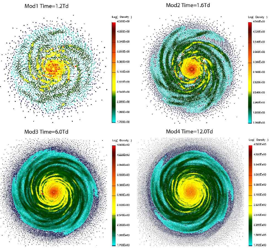
Figure 2: The particle distribution for the mod series of simulations at the end of each simulation. At the times shown, filamentary spiral structures have developed throughout the disks and are visible as azimuth varying blue, green and yellow color variations in the images. The three lowest resolution realizations have also produced a number of clumps (visible as red dots in the image) typically containing as many as several hundred individual SPH particles. Clumps in the mod3 realization are visible at about the 9 o’clock position in the figure, while in the two lowest resolutions, they are distributed throughout. The highest resolution realization produced no clumps. The color scale shown defines the base 10 logarithm of the surface density.

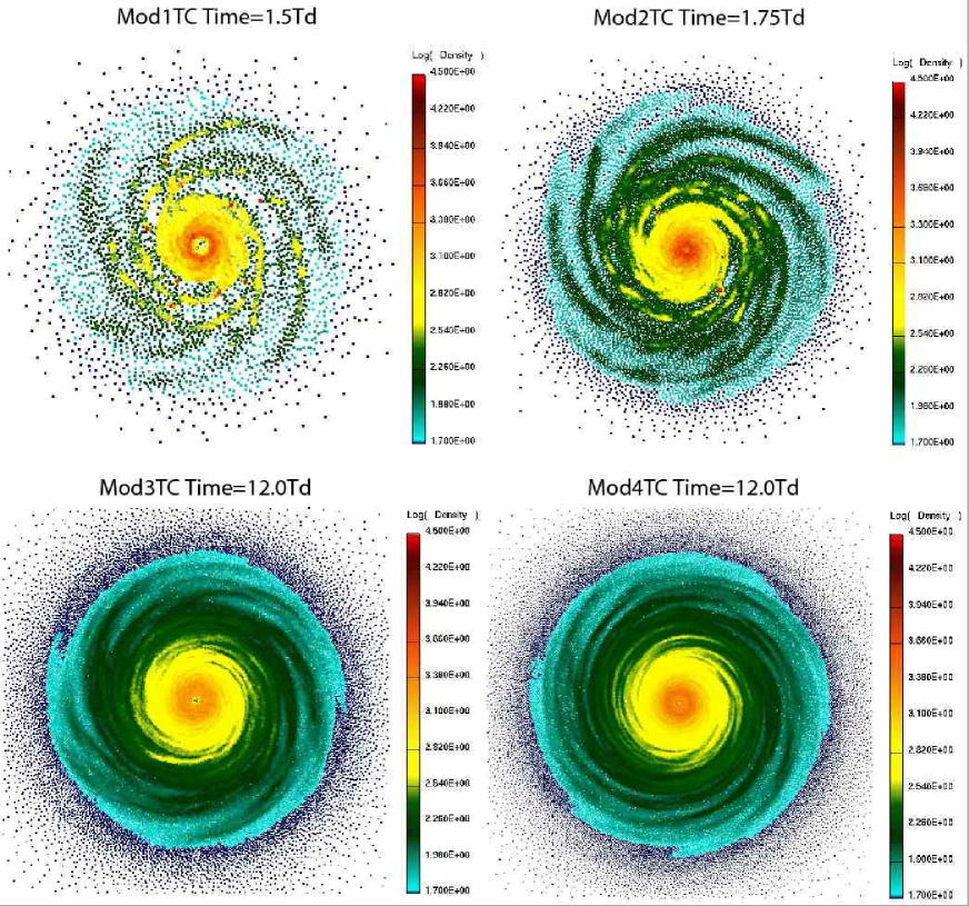
Figure 3: The particle distribution for the mod series of simulations with the TC92 kernel derivative, each at the end of each simulation. As in figure 2, filamentary spiral structures have developed throughout the disks and are visible as azimuth varying blue, green and yellow color variations in the images, with clumps (in the two lowest resolution realizations) visible as red dots in the image. The color scale is the same as in 2

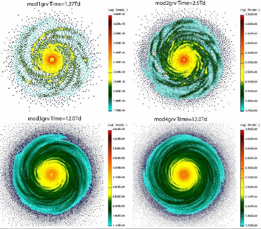
Figure 4: The particle distribution for the mod series of simulations with the alternate gravitational softening, each at the end of each simulation. As in figure 2, filamentary spiral structures have developed throughout the disks and are visible as azimuth varying blue, green and yellow color variations in the images, with clumps (in the two lowest resolution realizations) visible as red dots in the image. The color scale is the same as in 2

Using the conditions defined above, we ran a set of four simulations with varying resolution using each of three treatments for the small scale interactions between particles, but otherwise identical. The first treatment, with simulations labeled mod1-mod4 in table 1, uses gravitational softening of the form defined by equation 19 and the standard kernel gradient defined derived directly from equation 17. The second treatment, with simulations labeled mod1TC-mod4TC, uses the modified kernel derivative defined by equation 18 to determine mutual pressure forces between particles, again with the standard kernel softening. The third treatment, with simulations labeled mod1grv-mod4grv, uses the modified gravitational softening defined in equation 21 with the standard kernel gradient. Figures 2, 3 and 4 show these four realizations of the model, each at the termination of the simulation.

Each model develops multiple armed spiral structures over most of its radial extent, as in the previous Nelson et al.  (1998) work. The spiral structures are filamentary and change the details of their appearance as the simulation proceeds. Evolution after the formation of the spiral structure however, was strongly dependent on the resolution employed. In evolution of the three lower resolution realizations of the mod series, spiral structures eventually fragmented into multiple clumps, as in the Nelson et al.  (1998) work. The time at which clumps begin to form, measured from the beginning of the simulation, was later at higher resolution than at lower. Moreover, fewer clumps formed in the higher resolution realizations than in the lower, and in the highest resolution realization, no clumps were produced at all: the delay before clumps begin to form has become longer than the duration of the simulation (12$T_{D}$, or about 4200 yr).

Similar statements are true of both the modTC and modgrv runs, though there are a number of important differences as well. Of particular interest is the fact that the structure seen in figures 3 and 4 is substantially smoother than in the corresponding panels of figure 2. The overall relative smoothness is also reflected in the number of clumps that form in each realization. Where the mod3 simulation formed several clumps, simulations with the two modified treatments mod3TC/mod3grv did not. Although each of the corresponding lower resolution realizations did form clumps, the number that formed was smaller in each case and delayed in time relative to the standard kernel versions.

Figure 5: The azimuth averaged and instantaneous maximum surface densities plotted as functions of distance from the star for the test model derived from a simulation from Nelson et al.  (1998), realized at four resolutions (the ‘mod series of simulations–see table 1), each at the end of the simulation. Each panel in this figure corresponds to the same panel as in figure 2.

Figure 6: The same as figure 5, but for the TC versions of the simulations. Each panel in this figure corresponds to the same panel as in figure 3.

Figure 7: The same as figure 5, but for the alternate gravitational softening versions of the simulations (‘grv’). Each panel in this figure corresponds to the same panel as in figure 4.

Figures 5, 6 and 7 show azimuth averaged, radially binned surface density profiles of the same models as shown in figures 2, 3 and 4, at the same times. Also shown are instantaneous maximum surface densities, defined as the maximum in each ring seen at the time shown. The average in each bin is weighted by the number of particles in the bin, with the width of each bin set to 0.02 AU. At small radii, accretion onto the star has depleted the initial power law density distribution, in each case by a differing amount due to the differing magnitude of the dissipation derived from the artificial viscosity included in the simulation (see Nelson et al.  (2000) for a discussion of this effect). Further out, a number of spikes are visible in the profiles, each corresponding to the radial location of a clump in the disk. The lowest resolution realizations display a very large number of clumps, while successively higher resolution realizations produce fewer, or none. Both the number of clumps that formed and the radial extent over which they are found are smaller when we use the two modified kernel treatments, compared to the standard form. Though not possible to see in snap shots of a single time, an important difference between the evolution with the standard and either of the modified kernel treatments is that the cumulative maxima in the latter case remain far lower than the former and also do not appear to increase over time. We believe that this near steady state behavior represents the correct evolution of the system, even if it were to be evolved further in time.

Figure 8: A histogram of the number of SPH neighbor particles found at a given separation, for four variants of the mod4 simulation, as labeled. The separation is normalized to the dimensionless variable, $v=r/h$, and the histograms account for all neighbors of all particles in each simulation.

What is the origin of the differences in the morphology between each series and the others? We postulate that it lies in the treatment of the small scale interactions between particles, and specifically in force imbalances between pressure and gravity that may be present. If so, we may expect distortions in the distribution of interparticle separations, relative to what may be expected and to what may be present with other realizations. Figure 8 shows histograms of the distances between all neighbor particles for each of the three realizations of the mod4 simulations, as well as a simulation with the same resolution and initial condition, but without self gravity. Each histogram bin is defined to be of width $\delta v=0.002$, and all neighbors for all particles in each simulation are accounted for in the histograms. On the scale of the smoothing length, we can approximate the surface density as constant. For a uniform density distribution in a 2D simulation, realized with a random distribution of particles, we expect that the number of neighbors to be found at a given separation to increase linearly with the separation itself. At large separations, we recover the linear behavior. At smaller separations, all four distributions depart from the linear proportionality because the assumption underlying the linear proportionality neglects the influence of interparticle forces. Due to the different treatments of the small scale interactions, some differences also appear in the neighbor distributions.

The most striking feature of the plot however is the behavior near $v=0$. In the standard case, a large number of particles actually coincide in space, while in each of the other three variants, none do. This coincidence represents an extreme example of Herant’s pairing instability discussed above, that develops due to the interparticle pressure vs. gravitational force imbalance at small separations. The pairing instability seen here is clearly not identical to that discussed by Herant however, since no pairing is present in the non self gravitating realization for which conditions are most similar to those discussed by Herant. The pairing is also not similar to the numerical instabilities seen by Imaeda & Inutsuka (2002) for the same reason.

Figure 9 shows that the number of paired particles continues to grow as the simulation proceeds. After 12$T_{D}$, more than 65000 pairs have formed from $>130000$ particles: of the $\sim 260000$ original particles, about half have become paired. The existence of paired particles means first that the effective resolution of the simulation decreases with time as more and more particles become paired, and is consistent with our qualitative observation above that the cumulative maxima in these simulations also increased. Their presence also means that even though the force contribution from a single neighbor particle is small relative to the individual contributions from the rest of the system, when the particles approach coincidence the pairwise contribution can have an important and large scale influence on the behavior of the simulation. Based on these results, and the impact they have on the large scale disk morphology and its tendency to fragment, we conclude that using the standard kernel based gravitational softening in combination with the standard kernel derivative is likely to produce results contaminated with numerical artifacts in 2D simulations, and should not be used.

Figure 9: The number of particle pairs in simulation mod4 as a function of time. Corresponding figure for the other mod4 variants are not shown, since no particles become paired during their evolution.

3.3 Determining the resolution criterion

For each of the three series’ of simulations, the propensity of simulations to fragment decreased as resolution increased, until at sufficiently high resolution no fragmentation occurred at all. This behavior reflects that seen by Truelove et al.  (1997), where fragmentation was enhanced when resolution was insufficient, rather than that seen by BB97, where fragmentation was delayed. This is fortunate because it allows us to use the change in behavior of realizations of the same initial condition but differing resolution to determine empirically the approximate resolution (in number of particles) necessary to obtain ‘correct’ evolution. Specifically, we can apply the criterion to two simulations which straddle the boundary between those that produced fragments and those that did not. We can then note the value of $N_{\rm reso}$  at which the criterion succeeds for the entire simulation at the higher resolution, but fails for the lower resolution version. BB97 scaled the value of the Jeans resolution criterion through the value of $N_{\rm reso}$  as a multiple of the average number of neighbors, $\bar{N}_{\rm neigh}$. It will be convenient to scale the two dimensional criterion similarly here although in both cases, the correct measure will be a quantity independent of the specific neighbor count. We also note that in two dimensional SPH simulations, it is usual to use a smaller number of neighbors for each particle due to the lower dimensionality. In this work, we have used a number ranging between 10 and 30, depending on the local flow (see Benz, 1990, for details). We therefore scale by a factor $\bar{N}_{\rm neigh}$$=20$ for these simulations.

Figure 10: The cumulative maximum surface density reached at each point in the disk, binned as a function of radius in the mod3 and mod4 simulations. For reference, the azimuth averaged surface density shown in figure 5 as well (lower curve). The three smooth curves show the condition from equation 11 with a value of $N_{\rm reso}$  of 20, 120 and 240 particles (top to bottom in each panel).

Figure 10 shows the cumulative maximum surface density binned as a function of radius, along with the maximum resolvable surface densities determined from equation 11 using three values of $N_{\rm reso}$ equal to 1, 6, and 12 times the average number of neighbors for SPH particles evolved in 2D (i.e. 20). The cumulative maximum for each given bin is defined as the maximum surface density achieved by any particle in that bin over the entire course of the simulation up until the time shown.

For the mod3 realization, the cumulative maximum exceeds the critical value using the $N_{\rm reso}$$=$12$\bar{N}_{\rm neigh}$  criterion for all radii inside $\sim 20$ AU. At the same time, the $N_{\rm reso}$$=$6$\bar{N}_{\rm neigh}$ criterion is not violated except at a few localized radii. Interestingly, a small density spike relatively early in the simulation near 7 AU did not lead to clump formation, but later interactions near 10-15 AU did. For the mod4 simulation, the $N_{\rm reso}$$=12$$\bar{N}_{\rm neigh}$ condition is satisfied over the entire radial range for the life of the simulation, and no clumps formed. We can make only a tentative assignment of the value of $N_{\rm reso}$  from this result however because of the importance particle pairing may have on the effective resolution.

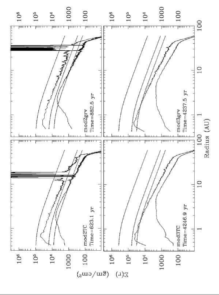
Figure 11: The cumulative maximum surface density reached at each point in the disk, binned as a function of radius in the mod2TC/mod3TC and mod2grv/mod3grv simulations. As in figure 10, the azimuth averaged surface density shown in figure 5 as well (lower curve) and the three smooth curves show the condition from equation 11 with a value of $N_{\rm reso}$  of 20, 120 and 240 particles (top to bottom in each panel).

Figure 11 shows the cumulative maximum surface densities for two of the simulations using the TC92 kernel derivative and the modified gravitational softening. In this case we plot the curves for mod2TC/mod3TC and mod2grv/mod3grv rather than for mod3 and mod4 in order to maintain the straddle of the fragmenting/non-fragmenting outcomes in these simulations. In both variants, the cumulative maximum densities in the mod2 realizations exceed the critical value using the both the $N_{\rm reso}$$=$6$\bar{N}_{\rm neigh}$ and $N_{\rm reso}$$=$12$\bar{N}_{\rm neigh}$ criteria, while the mod3 realizations obey the 6$\bar{N}_{\rm neigh}$ criterion but violate the 12$\bar{N}_{\rm neigh}$  criterion. Since no clumps formed during the evolution, the latter must be considered too conservative, and we conclude that the resolution required to avoid fragmentation due to unphysical growth of self gravitating structures in the disk is $N_{\rm reso}$$=$6$\bar{N}_{\rm neigh}$.

At first sight, the required resolution for the Toomre condition appears much larger in comparison to that for the Jeans condition analysis discussed by BB97. The apparent paradox is resolved if we note, as in section 2.2, that their assumed value of the Jeans mass was quite low and resulted in a relatively lower neighbor requirement. Our definition of the Toomre mass corresponds to an analogue of the larger definition of the Jeans mass defined as in equation 13.

The origin of the large required value of $N_{\rm reso}$  becomes clear when we observe that the values of the cumulative maxima (or indeed, also the slightly lower instantaneous maxima not shown) are typically a factor of several higher than the averages. Most of the difference can be accounted for by the existence of spiral structure in the disk, however fluctuations due to the effect of the exact, time varying positions of particles relative to each other on the calculation of the density make up a smaller, but still significant component of the difference. Such fluctuations are intrinsic to the SPH method itself and, while a small decrease is observable between the low and high resolution simulations in figure 10, their existence will be a part of all SPH simulations.

It is interesting to note that the densities can exceed the resolvable maximum in the lower resolution realizations for some time before clump formation begins. Further, the amount of time before the onset of clump formation is a resolution dependent quantity, with higher resolution leading to more time before clump formation. It is therefore clear that resolution studies are particularly important for particle simulations showing evidence of clump formation. Applying this statement to all three variants of our own mod series’ of simulations, it is clear that if clumps do indeed form in disks similar to those studied, the process requires a time scale than longer the 12$T_{D}$ ($\sim$4200 yr) for which we have evolved the system.

In the two lowest resolution realizations of all three variants (i.e. mod1/TC/grv and mod2/TC/grv), the numerical stability criterion is violated even in the initial condition. Since these simulations are only slight modifications from those presented in Nelson et al.  (1998) and at the same resolution, the same statement applies to those simulations as well. Regarding the clump formation seen in the simulations from that work, we originally concluded that although the physical model (in particular the isothermal equation of state) was insufficient to correctly model clump formation, if it was to occur at all, it would be most likely in between about 10 and 40 AU. The conclusion that the physical model in Nelson et al.  (1998) may be insufficient may indeed remain valid (see e.g. Nelson et al. , 2000)). However, the location and existence of clump formation is definitely invalid: it was due purely to failure of the Toomre criterion and not to any physical process, however modeled.

4 Fixed vs. dynamically variable gravitational softening in particle simulations

After investigating the effects of resolution and choice of kernel on disk simulations, in this section, we turn to an investigation of gravitational softening. We first discuss factors that motivate the selection of the value of a fixed softening length, then perform a side by side comparison of otherwise identical simulations employing either fixed or variable softening. Due to our conclusion in the last section that the standard softening/smoothing combination should not be used, we limit our investigations here to the TC92 and modified gravitational softening variants.

4.1 Choosing a fixed softening length

Unlike the case of variable softening, where the softening length is set locally and dynamically, with fixed softening the modeler must make a specific choice of the length that is appropriate for the entire simulation at all times. Choosing an appropriate value in disk models is substantially less trivial in the case of disk models than in the cloud collapse scenario discussed by BB97 because, simply as a consequence of the initial conditions (i.e. the density gradient as a function of distance from the central object), the smoothing lengths of particles are relatively steep functions of position. This is important because for any constant choice of softening, the relative magnitudes of softening to smoothing will also vary with position, perhaps artificially suppressing fragmentation in one region while enhancing it in another. Moreover, because the Toomre wavelength will itself be a function of radius through both density and temperature, both lengths will vary relative to it as well.

Naively, one might expect that variable softening could lead to results that are quite susceptible to small scale fragmentation. For example, if a region begins to collapse and the particles representing it approach each other, their mutual gravitational attraction continues to increase as their softening and smoothing lengths decrease, perhaps instigating the very problem softening is meant to avoid. It is not clear that such a condition exists in practice however. Variable softening was implemented for both of our mod series of simulations discussed in section 3.2, as well as our previous work in Nelson et al.  (1998, 2000). These models did not produce clumps, except as a consequence of insufficient resolution. On the other hand, fixed softening has been strongly advocated by Mayer et al.  (2002, 2004) and both their lower and higher resolution simulations do produce clumps.

There are a number of questions that we must answer in order to understand the implications of the softening choice and magnitude on the outcome of a simulation. First, since we have no a priori knowledge of where in the disk we may expect fragmentation to occur, if it is to occur at all, we must decide how to choose a value for the gravitational softening that allows the best reproduction of the real system. Given such a choice, what is the difference between the influence that fixed softening has on the simulation compared to variable softening? For example, to what extent can one or the other choice suppress fragmentation in models where it should not occur, but which may be under resolved? To what extent are physically valid evolutionary signatures also suppressed? Can one or the other choice actually instigate fragmentation in models that are otherwise stable? Can some values of fixed softening length both artificially suppress and enhance fragmentation in different parts of the same disk?

4.2 The influence of fixed softening on fragmentation in simulations with insufficient resolution

In this section, we investigate the influence of particular fixed values of the softening with a series of simulations (denoted the fix TC and fix grv series in Table 1) that are identical to the mod2TC and mod2grv simulations which we have shown to be unstable to numerically induced fragmentation with variable softening. These simulations implement a fixed softening using the same SPH spline kernel as is used for the hydrodynamic evolution, but are run, in the first case, with the modified kernel derivative for the pressure force calculation or, in the second case, with the modified 2D softening. Each of the four pairs of simulations uses a different softening length corresponding to the magnitude of the initial smoothing length at different locations in the disk. These are, respectively, the inner disk edge (0.5AU), the orbit radius corresponding to the region most susceptible to clump formation (15AU), and near the middle of the radial span of the disk (30AU), and its outer edge (50AU).

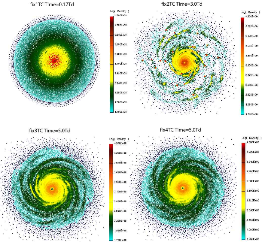
Figure 12: The particle distributions for the fix TC series of simulations, at the end of each simulation.

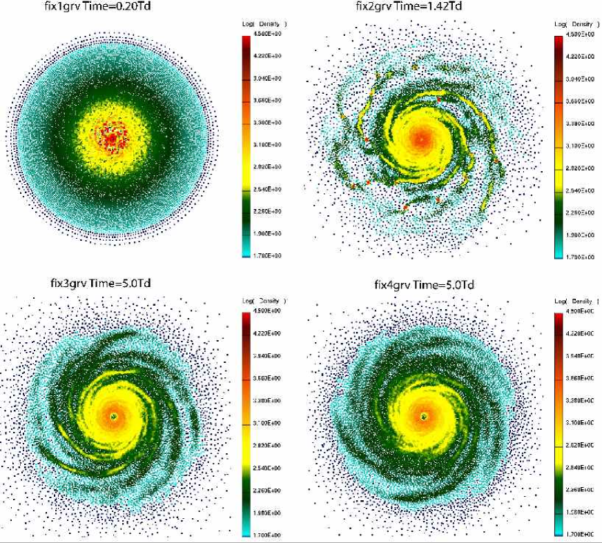
Figure 13: The particle distributions for the fix grv series of simulations, at the end of each simulation.

Figure 14: Azimuth averaged and cumulative maximum surface densities (as defined for figures 5 and 10) for the fix TC simulations, each defined with different, fixed gravitational softening lengths, and which are unstable to numerically induced fragmentation. The smooth solid curve represents critical surface density defined by the equation 11 with $N_{\rm reso}$=6$\bar{N}_{\rm neigh}$. The vertical dotted line in each figure corresponds to the radius at which the gravitational softening and the initial hydrodynamic smoothing lengths for the particles are equal.

Figure 15: The same as figure 14, but for the fix grv series.

We show the mophologies of these simulations in figures 12 and 13, and the azimuth averaged surface densities in figures 14 and 15. Overall, the behavior and morphology observed for each variant is quite similar to that of the other. With small softening (fix1TC/fix1grv) fragmentation occurs at essentially all orbit radii, on the same time scale as required for the disk itself to become active. Due to this rapid onset, we terminated it very soon after it began, so that radially more distant parts of the disk simply had insufficient time to become active. We believe that fragmentation would occur there too if the simulation were to be evolved further. Only at the inner disk edge, where the softening and smoothing lengths become comparable, is fragmentation suppressed. At all other locations, it is actually enhanced relative to the case of variable length softening shown in the mod2TC/mod2grv simulations above, where clumps only occurred at much larger radii. The fix2TC/fix2grv pair of simulations were evolved for longer in time than the corresponding mod2TC version, but ultimately they too produced clumps. Fragmentation occurred only in the region exterior to $\sim 15-20$ AU, where softening was smaller than smoothing.

In the fix3TC/grv pair, evolved with a still larger softening, strong spiral structures developed in the outer half of the disk, while comparatively weak spiral structure developed closer to the star. Significantly, the disk was evolved for 5$T_{D}$  and did not produce any clumps over that time. For simulations fix4TC/fix4grv, with the largest softening, spiral structure is largely suppressed throughout the entire disk, relative to their smaller softening cousins and to mod2TC. The gross structure of the spiral arms that form also appear somewhat weaker than those in the mod2TC/mod2grv simulations, however in the absence of a quantitative analysis of the pattern amplitudes (beyond the scope of this work) this statement remains somewhat subjective.

From these simulations, we can make the rather unsurprising conclusion that with a large enough softening value, clumping can be suppressed in simulations where it would otherwise occur due only to insufficient resolution. While not surprising, it is still important to quantify the both the value of ‘large enough’ and what changes in behavior occur as a function of gravitational softening, in order to be able to separate out real and artificial effects. In this case, ‘large enough’ gravitational softening appears to be larger than the hydrodynamic smoothing lengths in each part of the disk. In order to completely suppress clumping, softening must therefore be set comparable to the smoothing values in the outer part of the disk.

4.3 Enhancement of fragmentation in simulations with sufficient resolution

While we have seen that large enough softening can alter the behavior of an already numerically suspect (under resolved) simulation, it is also important to determine its effect on what might otherwise be considered a well resolved simulation. To investigate this question, we have run four simulations, denoted m1fxTC, m4fxTC, m1fxgrv and m4fxgrv in table 1, with identical initial conditions and resolution to our mod4TC/mod4grv simulations, but with fixed gravitational softening. As in the last section, the value of the softening is set approximately to the value of the hydrodynamic smoothing length at a predetermined radius in the disk. For the m1fxTC/grv pair of simulations, we set the softening equal to the smoothing at the inner edge of the disk (0.5 AU), so that they correspond to higher resolution versions of the fix1TC/grv  pair. For the m4fxTC/grv pair, we set the softening equal to the smoothing at $\sim 15$ AU. These simulations also correspond to high resolution versions of the fix2TC/grv simulations.

Figure 16: Azimuth averaged and cumulative maximum surface densities for the two simulations using the TC kernel derivative (left) and the two with 2D softening variant (right). In each case the gravitational softening length is fixed to the smoothing length at the inner edge (top) of the disk or at 15 AU (bottom), and all realizations are expected to be stable according to the Toomre criterion defined by equation 11 with $N_{\rm reso}$=6$\bar{N}_{\rm neigh}$. The vertical dotted lines correspond to the radius at which the gravitational softening and the initial smoothing lengths for the particles are equal.

Figure 16 shows the azimuth averaged and cumulative maximum surface densities for the two TC92 simulations. In contrast to the mod4TC/grv realizations, the two m1fx realizations produce fragments in the disk in much less than 1$T_{D}$. As for their lower resolution cousins, fix1TC/fix1grv, we terminated the simulations quite soon after they began due to the fragmentation. We expect that had evolution proceeded further in time, fragmentation would have occurred in the outermost parts of the disk as well. Consistent with our finding in section 3.2, that higher resolution realizations produced fragments later than lower resolution realizations of the same initial condition, fragmentation occurred later than in the fix1 variants. Fragmentation was delayed longer in the TC92 variant and was suppressed over a slightly larger portion of the inner disk.

In both cases, fragmentation only occurred in regions where the fixed gravitational softening was smaller than the hydrodynamic smoothing, consistent with the expectation from the discussion in section 2.7 and in BB97 for 3D simulations. Even though the relative size of the softening and smoothing lengths were the same in the low and high resolution realizations, clumps appeared only at somewhat larger orbit radii than at lower resolution. In all cases, the maximum surface densities in and near the clumps exceed the critical value determined from equation 11 and must therefore be considered to be numerically induced rather than due to physical processes.

Results in the m4fxTC/m4fxgrv simulations, with a much larger softening length, were quite different from each other: fragmentation did not occur with the modified kernel, but did with the modified softening, again in the outer part of the disk where interparticle force imbalances favored gravity over pressure. Although we have not shown the earlier evolutionary history of the m4fxgrv simulation, we note in passing that its character was markedly different than any other discussed in this work. High amplitude, filamentary spiral structures developed in the outer disk as early as $\sim 1$$T_{D}$, much earlier than fragmentation occurred as defined by a violation of the Toomre criterion. Although the structures developed with some regularity, they were unable to remain distinct, instead becoming progressively more sheared out, as they disappeared into the background flow. Based on this behavior, we conclude that the softening length chosen for this simulation was very near the boundary between enhancing and suppressing fragmentation, as we saw for the fix2grv/fix3grv simulations at lower resolution.

Figure 17: The number of multiple particles in the m1fxgrv (solid) and m1fxTC (dotted) simulations as a function of time. The two curves ending near $4\times 10^{4}$ represent the number of particle pairs, while the lower pair of curves represent particle triples.

If, as we have suggested, small scale interparticle force imbalances enhance fragmentation when the imbalance favors gravity, then we should expect simulations with fragmentation to contain a significant number of both paired particles and particles at small mutual separations, but few or none in simulations that do not fragment. Figure 17 demonstrates that indeed, this supposition is true for the two smallest softening length variants. The number of paired particles rises immediately and dramatically from zero to over $4\times 10^{4}$ over the short span of each simulation. Further, while the number of pairs appears to level out or even decrease at late times, the feature is actually a consequences of the increasing prevalence of higher order multiple particle groupings, such as triples or quadruples, as demonstrated by the lower pair of curves in the figure, representing the population of triples.

Figure 18: Histograms of the neighbor separations for all neighbors of all particles in the m4fxTC (top) and m4fxgrv (bottom) simulations.

Figure 19: The number of particle pairs present in the m4fxgrv simulation as a function of time.

Figure 18 shows histograms of the full neighbor distributions of the two larger softening variants and figure 19 shows the number of pairs as a function of time for the m4fxgrv simulation. As we suppose, a significant population of pairs and near pairs (i.e. with $v\la 0.1$) develops in the modified softening variant, which fragmented, while few do in the TC92 variant. Over the course of 12$T_{D}$, only a tiny population of near pairs developed compared to its cousin, and we observed only $\sim 5$ particles to become paired, a small enough number to be unimportant overall. While force imbalances must have been present at small separations in both models, we conclude that the enhanced interparticle pressure forces in the TC92 model, coupled with the higher resolution, were of sufficient magnitude to eliminate the numerically induced fragmentation that occurred when the softening length was smaller.

In an apparent contradiction of our supposition, the total number of paired particles generated in the three simulations here, which fragmented, is smaller than in the mod4 simulation, which did not fragment. Although we have made no quantitative comparison, a brief inspection indicates that the contradiction may be resolved by accounting for the spatial distribution of pairs and of near pairs. Because the small softening simulations were not evolved for a long enough time to become fully active, the distribution of pairs is quite concentrated in the regions did become active and did fragment, relative to the distribution in the mod4 realization where pairs are found spread much more evenly throughout the system. The m4fxgrv simulation, which did become fully active, generated many fewer pairs but did generate a large population of near pairs, indicating again the consequences of force imbalances favoring gravity. Given that the effective resolution in the mod4 run is decreasing with time, we expect that if it were to be evolved further, and the concentration of paired particles increased further, fragmentation would occur.

Disks realized with small fix softening fragmented in both the TC92 and the modified softening variants, and both in their low resolution realizations and at resolution high enough to satisfy the Toomre condition defined in section 3.3. An immediate conclusion from the similarities might be that, since the fragmentation occurred each realization, the simulations are in fact converged. While this conclusion may in fact be correct, it would also be seriously misleading. Due to flaws in their design, the simulations converge to an incorrect result. Interpretation of that result in terms of the physical behavior of the system and the importance of other correctly implemented physical processes becomes difficult or impossible. While the result and its invalidity may be clear in cases like our test simulations, the same statement may not be true in other simulations where the results are more difficult to verify. As a trivial example, the high and low resolution variants with larger fixed softening for which both low resolution variants fragmented, but only one at higher resolution. Our conclusion in this case must be limited only to the fact that the TC92 kernel modification is more likely to suppress fragmentation than the softening modification.

Two other, more technical aspects of simulations with fixed gravitational softening deserve mention. First, the cpu time required to run simulations with large, fixed softening to some specified time is far longer than with either the variable softening case or the cases with small, fixed softening. The reason is that with a large softening length, the interparticle spacing requires that a much larger fraction of the total number of gravitational interactions between particles be calculated as ‘atoms’ rather than grouped together as nodes, as is ordinarily done in tree-based gravity solvers in general use for particle simulations. Secondly, in cases where fragmentation does occur, a simulation with large fixed softening can proceed for much longer in time, because the time step size does not decrease nearly as much as occurs in a variable softening simulation at the same resolution. Continuing a simulation for a long time after clumping occurred and the resolution criterion has been violated would be of limited utility however, since the clump may cause large perturbations to the rest of the system that would not occur otherwise.

4.4 Recommendations for choice of softening

We conclude from our models that a fixed softening may either enhance or suppress density inhomogeneities depending on the specific choice of softening value relative to the hydrodynamic smoothing. No single value of softening may be considered ‘optimal’ in a disk with a large radial extent. In the extreme case, an incorrect (too small) softening value may induce fragmentation to occur in a simulation that would not, given another fixed choice or a variable softening set to the hydrodynamic smoothing length. Given an incorrect but too large value, suppression of physically correct structure may occur. In contrast, while a variable gravitational softening length may produce some violation of energy conservation, in the examples shown here the outcomes of the simulations are not affected in a manner as drastically as with fixed softening. We therefore recommend that simulations involving self gravitating hydrodynamic systems incorporate a spatially and temporally variable gravitational softening, whose length scale is the same as that over which the hydrodynamic quantities are smoothed.

Our recommendation is similar to, but stronger than that made by BB97 because we observe that fragmentation may develop in simulations whether or not the Toomre criterion (equation 5 or 11) is satisfied. Rather than signaling a temporal endpoint, beyond which BB97 conclude that evolution towards some final collapsed state is under resolved, we find that force imbalances at small particle separations can alter the evolutionary trajectory of a system which would otherwise never approach gravitational instability into one that does. Given that BB97 did not specifically study systems starting in a dynamically stable equilibrium condition for which fragmentation is known not to occur, as found in our disks, the behavior we observed in our simulations may not have been observable in their work. We suggest that it is independent of the specific system being simulated, and in fact applies to the Jeans collapse situation as well. Our conclusion is also consistent with that of Dehnen (2001), who made a detailed study of the effects of various choices of softening on the force errors produced by a static distribution of particles, and who recommends spatially variable softening in that case as well. Since in nearly all particle based hydrodynamic simulations, however, the smoothing length is not fixed in time, our recommendation goes beyond Dehnen’s study of a static distribution to including temporal variation as well.

We base our recommendation on the results of our simulations and on the following argument. Completely independent of whether or not either the gravitational or pressure force actually can be resolved on better or worse length scales than the other, is the consequence of the assumption underlying both softening and smoothing. Namely, an error in the net force is present by assumption when the contribution from either source is not fully resolved. We therefore have only the choice of how to handle this error most gracefully in the code. We submit that avoidance of large force imbalances in regions that are by definition under resolved is a trait much to be desired in the properties of the code because pathological behavior that results from such imbalances–artificial fragmentation or suppression of physically realistic fragmentation–are avoided.

Such a recommendation is not without cost however because it is equivalent to recommending that simulations using SPH should not require that energy be conserved. Although we have not attempted to quantify the magnitude of the violation, in general we believe it to be a relatively small component of the total energy of a given particle since only neighbor particles will contribute. Also, the violation will be smaller in higher resolution simulations because those neighbors will represent a proportionally smaller component of the total mass in the system, from which the potential energy of a given particle is derived. Finally, the fact that the gravitational forces and potential are approximated by a summation of terms derived from a tree search already violates strict energy conservation. Given the large body of literature using such approximations, often checked for veracity against other methods or observations, it would appear that few, if any, unacceptable consequences originate from a low level of violation. Assertions such as these are no replacement for a measurement however, and we refer the reader to Benz (1990) for discussion of a method to make an approximate quantification. We are also aware of current work, developing on the techniques discussed in Price & Monaghan (2004) and by the same authors (Price and Monaghan 2006, submitted), to create an SPH formulation that allows variable softening, while still conserving energy. Adapting SPH codes in existence to utilize this technique would appear to be highly desirable, since it would remove the most serious drawback of variable softening.

We have considered and discarded a third, intermediate softening option, in which the gravitational softening of each particle is set, for example, to the initial value of the hydrodynamic smoothing length, and is thereafter fixed. Although no specific tests have been performed to study this question, we believe that using such a prescription will yield results similar to the fixed softening case with a small softening length. For example, a particle initially located in a dense region (small softening value), which later moves into a less dense region (larger softening value) could act as an attractor for other particles in its current neighborhood. An exactly opposite effect might be seen for a particle initially in a low density region which moves to a high density region.

Secondarily, we question the aesthetic utility of such a prescription because it implies knowledge of the internal mass distribution of each particle that is both independent of any hydrodynamic expansion or contraction of the gas (the assumption underlying a temporally variable softening) and needlessly complex. The complexity is due to the fact that using constant, individual softening lengths suggests that information is known about not only the internal mass distribution of particles taken as an ensemble, but also the information that each particle has a different internal mass distribution from every other. We can postulate no circumstances where such exquisitely detailed information is likely to be available.

5 Simulations in 3 dimensions and/or using grid methods

The wave analysis underlying our resolution criterion makes the assumption that the flow is two dimensional: an integration over the $z$ coordinate is assumed. The test problem defined in section 3 was chosen to be similar to the models originally employed by Nelson et al.  (1998), and was therefore performed in the same two dimensional approximation as the originals. This approximation has historically been common in other works as well. In this section, we examine methods for applying the criterion to fully three dimensional models, and to the question of whether 3D simulations require additional constraints on resolution in order to ensure their accuracy.

5.1 Calculating surface density in 3D simulations

For fully three dimensional simulations, where a surface density is not directly available, the Toomre criterion cannot be applied without some additional computation. For grid based simulations, the computations are trivial and involve only an integral of the volume density in the $z$ direction. In cylindrical or Cartesian coordinates, for example the integral would pass to a summation of $\rho_{k}\delta z$ over a set of grid zones with spacing $\delta z$, with $\rho_{k}$ being the volume density in the $k$th grid zone in the $z$ direction.

For 3D SPH simulations, the computation of a surface density is more complex because there is no grid. Instead, we recommend the creation of a temporary grid onto which the volume density can be mapped. Then the surface density can be computed as a summation in the $z$ direction as in the case for grid based simulations. In test models, we have found good results by using a mapping to the grid based on the same smoothing technique used to determine the volume densities at the particle locations, for the mapping. At the location of each grid zone, we determine a list of ‘neighbor’ particles which may contribute to the density of that zone, then we use the formula

$$\rho(i,j,k)=\sum_{\rm neighbors}m_{p}W(r,h)$$ (26)

where $m_{p}$ is the mass of each neighbor particle, $W$ is the smoothing kernel, $r=|{\bf r_{p}}-{\bf r_{\rm zone}}|$ is the distance between the particle and the grid zone at location $(i,j,k)$ and $h$ is the mutual smoothing length of the particle and zone, defined as $\max(h_{\rm zone},h_{p})$. The grid smoothing length is defined as

$$h_{\rm zone}=\sqrt{\delta r_{i}^{2}+(r_{i}\delta\phi_{j})^{2}+\delta z_{k}^{2}}$$ (27)

where the components are the grid spacing in each of $r$, $\phi$ and $z$. We include a smoothing length for the grid itself in order to ensure that every particle contributes to at least one grid zone even in the case of vanishingly small smoothing lengths.

For the test problem discussed in sections 5.3, 5.4 and 5.6 below, we map the volume density onto a cylindrical coordinates grid where the radial coordinate is logarithmically spaced and the azimuth coordinate is uniformly spaced so that its spacing is $\delta r\approx r\delta\phi$ everywhere. In order to resolve the smallest scale features of the flow, we have chosen our grid resolution so that its spacing is comparable to the smallest smoothing lengths in the calculation. This grid spacing will in practice over resolve the features of most of the flow, and will not strictly be required in most circumstances. Our choice is motivated by the desire to ensure that the choice of grid (i.e. $h_{\rm zone}$) will contribute negligibly to the derived densities and the quality of the fitted quantities in our analysis that depend on them. In any case, the computational expense of choosing of a finely spaced grid for the mapping is small in terms of the time to run a simulation because the mapping is not required for the simulation itself, but only for post-processing.

A conceptually simpler mapping would be to use a Particle in Cell technique to assign the mass of each particle to the grid cell that contains it, thus determining a volume density for that cell. Unfortunately, we cannot recommend this method because it is susceptible to large errors due to the fact that SPH particles may have smoothing lengths much different than the grid spacing. For example, when a particle’s smoothing length is larger than the grid spacing, it should contribute to the density over a larger region than assumed by the PIC technique.

5.2 An unwarranted approximation: $\rho=\Sigma/2H$

When two dimensional simulations are performed, it is common to obtain an approximation to the volume density by dividing from the disk’s surface density by some factor multiplying the disk’s scale height. For an non-self gravitating isothermal gas, the factor will be $\sqrt{2\pi}\approx 2.5$ (see section 5.3 below), but will vary slightly depending on the exact input physics. For purposes of this section and for simplicity, we shall assume a factor of two exactly. As discussed at the end of section 2.4, the Jeans or Toomre stability criteria may be applied using this conversion to obtain one or the other of surface or volume density as required. In this section, we will investigate the impact that this conversion may have on the indirectly obtained values used in the Jeans criterion. We will refer here to the criteria directly applied through the use of equations 2 or 8 as the Jeans or Toomre criteria, while the criteria applied through the use of the disk scale height to convert surface to volume density (or vice versa) as the approximate Jeans or Toomre criteria.

In order to proceed, it is necessary to examine the results of a simulation modeled fully in 3D, so that both volume density and surface density are known. In one of a series of papers studying fragmentation in disks, Boss (2002) discusses 3D disk models and Boss (2004) continues this study with a close examination of the properties of a few models (primarily the model named ‘edh’) from the earlier work. We will use these models as a test bed for our investigation. Since our study has not specifically defined a value for $T$ in equation 5, we will assume that its value is $T=1/4$, which is identical to the value of $J$ required for Jeans collapse simulations. While we believe this to be a reliable assumption, only by examining the results of a specifically chosen test problem can we be fully confident that the value is sufficient. The consequences of the uncertainty in specifying $T$ are that comparisons between the magnitudes of $T$ and $J$ and the critical lengths associated with them, may be more difficult to interpret. In this section however, we seek primarily to test the veracity of the approximate forms of the criteria compared to the exact forms, and the absolute magnitudes are less important.

Boss’s model consists of a circumstellar disk modeled between 4 and 20 AU, evolved on a grid of $100\times 23\times 256$ (or $\times 512$ in some simulations) zones asymmetrically distributed primarily near the disk midplane. He includes an ideal gas equation of state and radiative cooling in the diffusion approximation, but omits an artificial viscosity, thereby omitting the viscous and shock heating modeled by it. With this model, he evolves a disk for 345 yr, at which time the simulation begins to violate the Jeans criterion due to onset of clump formation, and is terminated. We will apply our stability criteria to this model using each of the four relevant versions discussed in section 2.3.

Figure 20: (a) Critical wavelengths for the Boss (2002) simulation along the radial column including the forming clump. The exact Jeans and Toomre criteria are shown with heavy solid and dashed lines respectively, while the approximate Jeans and Toomre criteria (as defined in the text) are shown with light solid and dashed curves, respectively. The horizontal solid line, defines the spacing of the grid on which the system was evolved. (b) The ratio of the Jeans and Toomre wavelengths to the isothermal scale height ($H=c_{s}/\Omega$) as functions of orbit radius.

The top panel of figure 20 shows the value of the critical wavelengths at the time the simulation was terminated, using each of the four applicable implementations of the stability criteria. The failure of the Jeans criterion was used to define the end of the simulation, so its minimum value matches the grid spacing very closely. The exact Toomre criterion yields a critical wavelength that is about 30% smaller than that from the Jeans analysis. Using it and assuming that $T=J$, the model has already passed the boundary beyond which it becomes numerically suspect. Due to the speed at which clumping occurs, once underway, we do not believe that this small difference is very significant however, except to note that the simulation would have been terminated slightly earlier and at a lower density. At all other locations, the Toomre wavelength exceeds the Jeans wavelength and the evolution of the Boss simulation leading up to its termination passes the resolution test. The conclusions made from it stand on valid numerical grounds according to the Toomre resolution criterion.

On the other hand, the approximations of the Jeans (light solid) and Toomre (light dashed) criteria lead to critical wavelengths in the forming clump that differ by a factor of 1.56 larger than and 4.6 smaller than the grid spacing, for the approximate Jeans and approximate Toomre criteria, respectively. Moreover, using the approximate Toomre criterion, the simulation is already well past the time for which its evolution is numerically valid. Each of the approximate forms uses the isothermal scale height to render the conversion. Does this quantity remain relevant in a collapsing region?

The bottom panel of figure 20 shows the ratios of the Jeans and Toomre wavelengths to the scale height. Except near the forming clump, the Jeans wavelength is many times the disk scale height, making its application as a resolution criterion unclear according to the argument in section 2.3. The Toomre wavelength is also many times the disk scale height, but this only makes its application to a resolution criterion more appropriate, according to the same arguments. We therefore recommend that it be used in favor of the Jeans criterion in simulations of disks. In and near the collapsing region, both wavelengths become significantly smaller than the scale height. Since those wavelengths loosely define the physical size of the collapsing body, we can conclude that the structure of that object is no longer well represented as a slightly perturbed disk structure under which assumption the scale height was originally defined. Thus, the approximate criteria should not be used because their values become inaccurate near the clump, due to the fact that the disk vertical profile becomes distorted.

5.3 A simple 3D test problem to test the accuracy of the hydrodynamics in disk simulations

In section 2.8, we discussed the possibility that a disk simulation performed in 3D may not in fact be truly three dimensional because the disk thickness may be comparable to the smoothing lengths of the particles in and SPH simulation, or the grid dimension in a grid based simulation. Here we explore the consequences of such simulations using a simple test problem. Specifically, the problem of a non-self gravitating disk evolved with an isothermal equation of state. For this system, an analytic expression for the vertical structure of the disk can be derived exactly, and direct a comparison between the analytic result and theory can be made. This test problem is equally applicable to grid based simulations and to particle simulations, and we propose it as a general test for interested numericists.

The vertical structure of the gas in a non-self gravitating disk will obey the equation

$${{dp}\over{dz}}=\rho{{GM_{*}z}\over{(r^{2}+z^{2})^{3/2}}}$$ (28)

where $p$ and $\rho$ are the pressure and volume density, $z$ is the altitude above the disk midplane and $r$ is the cylindrical radius. For an isothermal equation of state, the pressure is related to the density and sound speed through the definition $p=\rho c_{s}^{2}$. Using the equation of state to replace pressure with density, the solution to the differential equation is

$$\rho(z)=\rho_{0}e^{-z^{2}/(2H^{2})}$$ (29)

where $H=c_{s}/\Omega$ defines the isothermal scale height and $\Omega=\sqrt{GM_{*}/r^{3}}$. For any given location in the disk, the surface density can be obtained by integrating equation 29 over all $z$, giving the relation

$$\rho_{0}={{\Sigma}\over{\sqrt{2\pi}H}}.$$ (30)

We use a modification of the 2D test problem described in section 3.1 for this test. Particle layout, temperature and surface density are defined as in the 2D problem, such that a minimum Toomre $Q$ value of $\sim 1.5$ would be obtained if self gravity were included. To obtain an initial $z$ coordinate for each particle, we use a Gaussian pseudo random number generator whose width is defined by the local value of the disk scale height, consistent with equation 29. Definition of the initial velocities takes account only of stellar gravity and pressure forces rather than disk self gravity as well. Velocities in the $z$ coordinate are set to zero.

Before proceeding further, it is significant to note that the specific model we propose is a step removed from those of greatest relevance for actual systems because vertical density distributions depend on the details of the physical model employed. Also, as a practical matter, the exact definition of ‘scale height’ itself can lose meaning in such models. To the extent that it does remain meaningful, any resolution requirement may be sensitive to the details of the model if, for example, a larger fraction of the mass were in an extended envelope or were concentrated closer to the midplane than with an isothermal structure, as is the case for the isentropic structure discussed in section 5.7 below. In the context of the spatial distribution of particles or grid cells that represent the mass and at a coarse level of examination, models that result in a higher midplane mass concentration will be somewhat similar in structure to colder isothermal disks in which the scale height is simply not as large. We therefore believe that any modifications to the critical resolution appropriate for other models will be not be large and proceed to define a criterion for isothermal structure that we believe will be generally applicable. In the following two sections, we will however, proceed to define a resolution criterion in two complimentary ways: as a requirement per scale height at the disk midplane, and as a resolution per vertical column, in order to facilitate its use more generally.

5.4 Results from simulating our 3D test problem with SPH

We have run a series of simulations modeling the 3D test problem at different resolutions, from $1.3\times 10^{5}$ to 10⁶ particles, each labeled sgoff3-6 and defined in table 1. We allow each simulation to run for two orbits of the outer edge of the disk in order to ensure that the configuration represents the true system as realized by the hydrodynamic code rather than any peculiarity of the initial configuration. We then map the volume density and velocities onto a three dimensional grid and calculate the surface density at each location. We pose the following question for the configuration, which must be answered affirmatively before the results can be validated: does the configuration generated by the simulation correctly reproduce the correct midplane densities and scale heights everywhere in the disk?

To answer the question, we generate least squares fits to the densities as mapped onto a temporary grid to compare to the analytical values defined by equation 29. Each fit returns three parameters corresponding to the values of $\rho_{0}$ and $H$ in equation 29. We limit the fits to the radial region between 1 AU and 45 AU in order to eliminate the possibility that conditions at the inner or outer boundary of the disk distort the true picture of the structure. Inspection of the disk structure shows that these limits ensure that the fits are limited to the regions where the rotation curve is unaffected by either the gravitational softening of the star at the inner boundary or large density gradients near the outer boundary. In order to remove any potential systematic errors derived from the resolution of the grid or simulation itself, we average the volume densities at each altitude over patches of approximately one scale height on a side, so that the same number of fits are generated for each simulation. Finally, in order to retain self consistency in the face of any evolution of the disk away from the initial surface density profile, we derive the analytic values for $\rho_{0}$ and $H$ using the locally determined value of the surface density and rotation velocity, through the relation $H=c_{s}/\Omega$ and equation 30.

Patches are defined in successive radial rings of the disk by the condition that a ring’s radial extent is the local, analytically determined value of the scale height. Their azimuthal extent is determined by the same condition, so that the total number of patches in a ring is defined by its circumference divided by the scale height. At the grid resolution chosen for the analysis, each patch covers a region of $\sim 200$ or more cells in the vertical coordinate, and $10\times 10$ radial and azimuthal grid cells near the inner disk edge where the scale heights are small, and $15\times 20$ near its outer edge where they are much larger. In total, approximately 14000 patches are required to cover entire disk, so that 14000 separate fits of the vertical structure in the disk are performed.

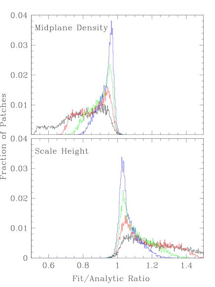
Figure 21: Histograms of the best fit midplane density, $\rho_{0}$ (top) and scale height, $H$ (bottom). The black, red, green and blue curves correspond respectively to the progressively higher resolution simulations sgoff3-sgoff6. The bins of the histogram are of width 0.25%.

Figure 21 shows histograms of the ratios of the fitted quantities $\rho_{0}$ and $H$ to their analytic predictions, normalized to the total number of patches. At the lowest resolution shown, the vertical structure in the simulation is clearly more extended vertically than predicted, with the distribution of scale heights extending more than 50% larger than the analytic values and the midplane density distribution extending nearly 50% below the analytic values. Both distributions are spread relatively evenly over the range extending from the most extreme under or over estimates on one end, to nearly the correct analytic value on the other. The distributions become narrower for each of the each of the higher resolution variants of the model, and appear in fact to be converging to the analytically expected values. However, even at a resolution of one million particles, the highest resolution in our study, the peaks of the distributions deviate from the analytical values by about 5% and a significant population of patches are best fit with midplane densities and scale heights as much as 20% below or above the analytic values, respectively.

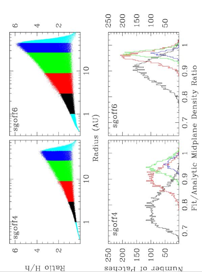
Figure 22: Top panels: Scale height to smoothing length ratio for all particles in the sgoff4 and sgoff6 simulations, as labeled. Bottom panels: Histograms of the ratio of the best fit to analytic midplane densities expected for all patches in the disks between 1 and 45 AU. The color of each histogram corresponds to to patches in the ranges 1–3 AU (black), 3–9 AU (red), 9–27 AU (green) and 27–45 AU (dark blue), as shown in the top panels. Patches at orbit radii smaller than 1 AU or larger than 45 AU (light blue) are excluded from the histograms in order to minimize distortions due to decreased resolution at the inner and outer disk edges. As in figure 21, histogram bin widths are set to 0.25%.

We can convert the correspondence between simulation and theory into a resolution requirement if we can quantify the minimum number of particles required in a vertical column for which the fit parameters are accurately reproduced. The top panels of figure 22 show the vertical resolution of the disks quantified as a ratio between the expected scale height and the smoothing length of each particle. The bottom panels show the quality of the reproduction of the analytically determined disk midplane densities as in figure 21, broken out into separate histograms for each of four radial regions of the disk.

The vertical resolution varies between less than one smoothing length per scale height in the inner disk to as many as six near the outer edge of the high resolution simulation, sgoff6. The ratio takes values over a range from less than unity up to a orbit radius dependent maximum value because particles located near the midplane at some radius, where densities are high, will have correspondingly smaller smoothing lengths. Particles located at higher altitudes where densities are lower will have larger smoothing lengths. Dividing each by the scale height (constant at a given radius) produces the range. The maximum value of the ratio varies as a function of orbit radius primarily because the scale height itself is a function of radius, through the combination of the predefined temperature profile (equation 22) and the rotation curve.

In the 1–3 AU region of the disk, the entire vertical structure of the disk is represented by the smoothing length of only a single particle. The exact positions of neighboring particles relative to each other therefore cause a correspondingly larger influence on the densities, as demonstrated by the very wide distribution of midplane densities present in both the sgoff4 and the sgoff6 realizations, relative to their analytic values. In each successively more distant region, and at both resolutions, the distribution becomes narrower and of better quality, demonstrating the value of the increased vertical resolution. For example, the vertical structure is resolved by $\sim 1-2$ smoothing lengths per scale height at $r\la 3$ AU, and the fitted midplane densities fall between 65 and 95 percent of their analytic value for the 260000 particle simulation and 75 and 100 percent in the 1 million particle run. At the other end of the spectrum, density fits fall within $\sim 5$% of their predicted values only in the two outermost regions in the high resolution simulations, corresponding to orbit radii $>9$ AU (i.e. the green and dark blue histograms in the figure), and only part of the distribution in the single outermost region of its lower resolution counterpart, corresponding to radii $>$27 AU.

If we specify that midplane densities within 5% of their analytic values are sufficiently accurate for the purpose of simulating the evolution of a circumstellar disk, then only these outer regions of the disk have sufficient accuracy. In the two best resolved regions of simulation sgoff4, ratios of fit to analytic midplane density values peak near $\sim 94-95$% and extend to as low as 90%, resolving one scale height with at most $\sim 3-4$ particles. In the same regions of sgoff6, The peaks of the distributions increase to near $\sim 96-97$%, with tails extending to as low as $\sim 92-93$%, resolving one scale height with as few as 3.5 particles at 9 AU and as many as 6 further out. We conclude that midplane densities within $\sim 5$% of their analytic values are achieved only in regions where the vertical structure of the disk is resolved with at least $\sim 4$ smoothing lengths per scale height at the disk midplane.

5.5 Interpreting the vertical resolution requirement at the disk midplane in the context of the full thickness of the disk

It is important to note that the requirement for $\ga 4$ smoothing lengths per scale height near the disk midplane is sufficient only for obtaining reasonably accurate midplane densities, and only for a mass distribution described by equation 29. Quantities at higher altitudes may still be significantly under resolved because smoothing lengths are larger there due to the correspondingly lower densities. Errors due to insufficient resolution at high altitudes will be of lesser importance for simulations modeling gravitational instabilities because the magnitudes of the pressure and gravitational forces important for fragmentation will be largest where the mass is concentrated, close to the midplane. Nevertheless, some particles must be present at high altitudes in order to compress those lower down to the required densities. How many are enough?

In this section we quantify the minimum number of particles required per vertical column needed to obtain good correspondence with theoretical expectations for density near the midplane in our models. Because it is a metric that is effectively an integral over a full vertical column, this quantification is likely to be much less sensitive to the exact distribution of mass over the column, and so more generally applicable than a quantification per scale height. It also eliminates the possibility of misperceptions based on the idea that the total mass outside the midplane is small enough to be neglected in estimates of the total resolution required per vertical column.

For the isothermal disks in this study, 98% of the disk mass will reside within three scale heights of the midplane, according to equation 29, meaning that the mass is effectively distributed over a total of six scale heights accounting for symmetry above and below the midplane. At the simplest level, we might therefore approximate the required vertical resolution to be $\sim 24$ smoothing lengths per vertical column to avoid serious errors in the midplane densities. A somewhat more accurate quantification might also account for the fact that mass is preferentially located near the midplane, with fewer particles present at high altitudes.

In principle, we can derive an approximate number of particles required per vertical column if we simply quantify the particle density over all altitudes in a single vertical column. At the minimal resolution required to obtain accurate midplane densities however, we must presume that the high altitudes remain inaccurate due to the fact that densities are much lower there and particle separations larger, and they may therefore remain under resolved. Any direct quantification of the resolution required based on the actual distribution of particles in a simulation would therefore suffer from the inaccuracies in their high altitude distribution.

A fact that allows the analysis to proceed is that, for the purpose of ensuring accurate midplane densities, only the total weight of particles at high altitudes is needed rather than their distribution. This is important because weight is a quantity integrated over the vertical column of material and will therefore take the same value whether or not the mass distribution responsible for it is well resolved. Any high altitude mass distribution yielding the same weight will yield the same midplane density so that, given a correct midplane density, we may infer that the total weight is approximately correct as well. We may therefore assume that the high altitude mass distribution derived from our simulations is correct (even though it may not be), for the purpose of converting densities at a given altitude to a corresponding number of particles needed to supply the correct compressional forces to midplane material.

We can quantify the total particle count per vertical column in the simulations using a modification of the patch averaging strategy used above. Rather than creating full 3D density distributions for each patch, it is sufficient only to quantify the averaged number of particles located in each, and to create a coarse vertical distribution of the particles by assigning each particle to a histogram bin according to its altitude. The result is the patch averaged volume density of particles in each histogram bin, from which a linear (vertical) particle density per scale height can easily be obtained by taking a cube root. A final link is to note that interparticle separations are $\sim h$ and that, by definition, the histogram bins are of width $H$, so that the linear particle density is equivalent to the ratio of smoothing length to scale height.

Figure 23: The patch averaged vertical, linear particle density binned in histograms of width $H$, for the sgoff4 and sgooff6 simulations. From top to bottom, the histograms in each panel correspond to the dark blue (solid), green (dotted), red (short dashed) and black (long dashed) regions as defined in figure 22. The numerical values associated with each curve are sums over all histogram bins thus defining the averaged total particle counts per vertical column.

Figure 23 shows histograms of the patch averaged ratios of $H/h$ defined using this procedure, separated into the same radial regions defined in section 5.4. Consistent with expectations based on the physical model and on the fit results above, each histogram displays a maximum at the midplane and non-zero populations to as high as $\sim 3-4$ scale heights in each direction. Histograms with larger net populations exhibit a progressively more peaked structure, reflecting the better agreement with the analytical model provided by the higher resolution. For the present purposes, it is interesting to note that in every region of the disk, the total resolution per vertical column is several times the resolution assuming that only the midplane contributes significantly to the total.

In section 5.4, we determined that only the two outermost regions of the sgoff6 simulation were well resolved in our simulations. Here, we see that on average, the resolution of vertical columns in these regions is $\sim 17$ and $\sim 22$ particles per column for the 9–27 AU and 27–45 AU regions, respectively. For the lower resolution sgoff4 simulation, the highest overall vertical resolution reaches $\sim 14$ particles per column, and all other regions in both simulations fall progressively farther below this value. Since fits in all of these regions deviate from the analytic expectation by more than 5%, we therefore conclude that a minimum of $\sim 17-20$ particles per vertical column are required to adequately reproduce the density structure at the disk midplane.

5.6 Significance of the results of the 3D test problem

In self gravitating systems, the exact balance of pressure and gravitational forces will tip that system towards or away from two dramatically different outcomes: fragmentation or continued smooth evolution. In marginally stable systems of interest to modelers, the exact balance between the two forces will be determined from terms of nearly equal magnitude, but of opposite sign. If one of those quantities is incorrectly calculated, the outcome will be dramatically different.

The results of the test above demonstrate that simulations with too few particles tend to underestimate the midplane densities, in the case of 2.6$\times 10^{5}$ particles, by as much as 30-35%. This is important because the pressure will be underestimated by a similar factor through the equation of state. Fragmentation will therefore be enhanced in an under resolved simulation compared to that of either a well resolved simulation or, more importantly, a real, physical system. Because we have not performed self gravitating simulations, we cannot specify the exact effects the errors will have in simulations or the level of enhanced fragmentation that may occur however. Such details are difficult to specify with precision because any enhancements may be mitigated in part by the fact that the cause of erroneously low densities in SPH is simply that particles separations are greater than they should be, so that gravitational attraction between them is correspondingly less. Any possibility of mitigation of this sort provides little comfort relative to simply solving the hydrodynamic equations accurately in the first place however.

For the disk morphology discussed here, resolution sufficient to accurately reproduce the disk’s vertical structure and midplane density beyond $\sim 10$ AU requires at least one million particles. Although we have not attempted to quantify the differences through simulations, colder disks closer to the fragmentation boundary will have correspondingly smaller scale heights, and will therefore require still more total particles to ensure adequate resolution.

For example, the disk scale height and $Q$ values both depend directly on the sound speed, so a change in one will be reflected proportionally in the other. A disk with minimum $Q=1.3$ or $Q=1.1$ will decrease the scale height below that in our simulations by a factor $1.3/1.5\approx 0.87$ or $1.1/1.5\approx 0.73$ respectively. In order to retain adequate resolution of the vertical structure, smoothing lengths must be decreased by a similar factor by increasing resolution. In 3D, the magnitude of the increase will be a factors of $1/0.87^{3}\approx 1.5$ or $1/0.73^{3}\approx 2.5$ corresponding to $\sim 1.5$ or $\sim 2.5$ million particles. No simulations of circumstellar disks in the context of planet formation have yet been performed at such high resolution.

Even at a resolution of 1 million particles, the vertical structure in our simulations is not accurately reproduced inside 10 AU, where midplane densities drop well below their analytic values. This is important for simulations of gravitational fragmentation because the Jovian planets in our own solar system formed at such radii. The erroneously low densities may lead to enhanced fragmentation in those regions, even if the structure is accurately modeled further out. Also, the resolved and unresolved parts of the disk are in no way isolated from each other. As waves or other structures propagate through the disk, their subsequent evolution will be perturbed by the change in resolution, so that the evolution throughout the entire simulation become suspect.

Both the small values of the scale height at small orbit radii and the insufficient resolution there are consequences of the $r^{-1/2}$ temperature profile assumed for the disk, and commonly used throughout the literature. Through the sound speed and rotation curve, the scale height will exhibit a proportionality $H/r\propto r^{1/4}$ and, for minimum $Q=1.5$, will take values of $\sim 0.025$ near 1 AU increasing to $\sim 0.065$ near 45 AU. The temperature profiles in our simulations reflect the stage of active disk evolution during which gravitational instabilities are most likely to be present. A temperature profile inversely proportional to radius will yield a flat profile and so avoid the issues of variable vertical resolution, but such steep profiles are not observed in real systems (Beckwith et al. , 1990), and so we discount them here.

5.7 Additional requirements on vertical resolution for simulations including radiative transfer

Above, we showed that the vertical structure of an accretion disk must be resolved with some minimum number of particles if mass densities in the disk midplane are not to be substantially underestimated. Although this requirement may be sufficient to ensure accurate simulations in the case when comparatively simple physical models are employed, it will be less so when radiative transfer is included. Here we describe an exercise meant to illustrate requirements for resolution of the high altitude structure of the disk, if serious errors in the cooling rates derived from radiative emission from the disk photosphere are also to be avoided.

At the orbit radii most relevant for planet formation ($\la 20$ AU), disks will be optically thick in the sense that the optical depth, $\tau$, calculated from infinite distance to the disk midplane is large. This is important because it means that the cooling rate of packet of disk material will be well modeled by a blackbody cooling law whose temperature is defined at the disk photosphere. If the altitude of the photosphere is known only approximately, due to low resolution or simple miscalculation, the cooling rate will be similarly approximate because the temperature structure near the photosphere is not known precisely. Comparatively small errors in temperature will lead to much larger errors in the local cooling rate because of the $T^{4}$ proportionality of the blackbody cooling function.

Accurate knowledge of the cooling rate and its associated photosphere temperature is important because the dynamical balance of heating and cooling processes in disks is quite precarious: most of the heating and cooling sources are capable of removing or replacing essentially all of the disk’s thermal energy over the course of only a few orbits (Durisen et al. , 2006). Specifically for the question of disk fragmentation, Gammie (2001) shows that cooling rates faster than $\sim 3/\Omega$, where $\Omega$ is the local orbit frequency, lead to disk fragmentation, but longer cooling rates may not in a local calculation. Later global calculations of Rice et al.  (2003) confirmed this result for low mass disks, where they found that a cooling time of $5/\Omega$ was long enough to prevent fragmentation, but a cooling time of $3/\Omega$ was not. Simulations of higher mass disks with cooling rates of 10 and 5 $\Omega^{-1}$ showed similar changes in behavior. From these results it is clear that an error in the cooling rate as large as a factor of two will be sufficient to suppress or enhance fragmentation in a simulation which would otherwise follow a very different evolutionary path. A error of factor of two in the cooling rate will be equivalent to an error of $\sim 20$% in the photosphere temperature, due to the $T_{eff}^{4}$ dependence of the cooling on the temperature. Since an error of such magnitude may seriously alter the balance between cooling and heating, a more restrictive limit must be set to ensure that any fragmentation that does occur is not subject to numerical error. If we set an arbitrary standard that a cooling rate accurate to 25% will be sufficient to ensure results are not contaminated by numerical errors, then we will in turn require a photosphere temperature accurate to $\sim 5-6$%.

Figure 24: Vertical density (top), temperature (middle) and optical depth (bottom) profiles of a disk at 10 AU, with local surface density of 500 gm/cm² and a midplane temperature of 50 K, using the model of Nelson et al.  (2000) to determine structure. The altitude coordinate is normalized to the value of the isothermal scale height $H_{\rm iso}$ determined at the midplane. Dotted and long dashed vertical lines on each curve are placed to straddle the photosphere surface at $\tau=2/3$ (horizontal dashed line), at distances of $H_{\rm iso}/10$ and $H_{\rm iso}/20$, respectively. Over these distance, the temperature deviates $\sim 15$% and $\sim 7$% above or below the true photosphere temperature.

Given the requirement as stated, it remains to convert the constraint on the photosphere temperature determination to a constraint on required spatial resolution of the vertical disk structure. One approximate model of the vertical structure of a disk is available from the work of Nelson et al.  (2000), in which an isentropic vertical structure is assumed, for a locally plane parallel, self gravitating disk. Figure 24 shows temperature and optical depth profiles as a function of altitude for a region of a disk expected to be interesting for disk fragmentation, derived from the Nelson et al.  2000 model. Several points are of interest in evaluating the figure. First, although the density structure follows an approximately Gaussian structure, at least in coarse outline, it is dramatically compressed relative to that expected for an isothermal disk. No material is present above an altitude of $\sim 1.7H_{\rm iso}$, due to the different physical assumptions employed in deriving the mass distribution. Second, this configuration is optically thick, with an optical depth to the midplane of $\sim 100$, meaning that a disk photosphere surface may in fact be defined.

For the purposes of evaluating the radiative energy losses, a third point will be of most importance. Namely, that near the disk photosphere surface both the density and temperature are changing rapidly with altitude. A calculation that resolves these profiles too coarsely will therefore also only coarsely resolve the photosphere surface itself, possibly exposing the hot disk interior to space. For example, if the particle density near the photosphere for an SPH simulation is such that smoothing lengths are $h\approx H_{\rm iso}/10$, then to a first approximation, the photosphere surface itself will be resolved on the same spatial scale because interparticle separations are themselves $\sim h$. A particle actually located anywhere within $h$ of the actual photosphere surface may be determined to define the photosphere surface, simply because no other particle happened to be at a higher altitude there. An identical argument holds for grid based simulations, with the size of a zone at the photosphere surface replacing smoothing length.

Figure 24 shows that uncertainties in the altitude of the photosphere surface of $\sim H_{\rm iso}/10$ results in an increase or decrease of the derived photosphere temperature of $\sim 15$%. Doubling the linear resolution to $\sim H_{\rm iso}/20$ decreases the uncertainties to $\sim 7$%, comparable to our requirement of errors no larger than $\sim-5-6$%. We therefore conclude that simulations including radiative cooling must resolve the disk photosphere surface at a spatial scale no coarser than $\sim H_{\rm iso}/20$, when structure models similar to ours are employed.

After completing the exercise and deriving this requirement, we must also immediately point out that the quoted required resolution is not universally applicable without modification. Any constraint on spatial resolution in the context of radiation will be considerably complicated by the fact that the vertical temperature profile will be significantly influenced both by preferential dissipation of shocks at high altitudes (Pickett et al. , 2003), by radiative heating by external sources like the central star (Chiang & Goldreich, 1997) and, if any remains at the time of the simulation, the surrounding molecular cloud. As Chiang & Goldreich 1997 also note, wavelength dependent opacities will also play a role, to the extent that long wavelength radiation is able to cool the disk interior effectively, even while shorter wavelength radiation remains trapped.

In spite of these cautions, we remain convinced that the above exercise remains a valuable illustration. It is based only on the condition that the transition between optically thick and optically thin material is well resolved and, although it is applied to a particular model of the vertical structure, it is not tied to it specifically. Given the overall gross vertical structure of disks, in which densities are high at the midplane and drop steeply as altitudes increase, optical depth profiles similar to that in figure 24 will occur in other models as well. Because the optical depth is a very steeply falling function of increasing altitude, the transition region will be narrow, as in the model above. Whether that narrowness can be translated directly into a constraint on the spatial resolution will depend on the details of the temperature profile there, and its influence on the accuracy of radiative energy transfer. The specific criterion as applied above presumes a temperature profile decreasing with altitude as the density decreases, $T\propto\rho^{\gamma-1}$. If instead a much flatter profile exists across the transition, a less restrictive criterion may still permit sufficiently accurate evolution.

6 Concluding remarks

After exploring the conditions required for simulations to produce numerically valid results, we turn now to summarizing those conditions, to comparing the work done here with previous work in the literature, and to commenting on additional requirements beyond numerics that are required for simulations to accurately reproduce the evolution of real systems.

6.1 Summary of our main results

Our first result is to extend the numerical criterion for the validity of simulations involving collapse in clouds and based on the analytic Jeans collapse formalism (BB97, Truelove et al.  (1997)), to the case of disk systems where the geometry of the mass distribution is both flattened and rotating so that the Jeans treatment is inapplicable. Whereas a minimum spatial resolution per Jeans wavelength or minimum number of particles per Jeans mass is required in the cloud collapse case for grid or particle based simulations, respectively, in simulations of disks we require a minimum spatial resolution per ‘Toomre wavelength’ or minimum number of particles per ‘Toomre mass’, for grid based or particle base simulations, respectively. The two forms of the new criterion are given in equations 5 and 11.

We also note that simulations failing to resolve one or the other condition yield quite different outcomes. In the case of the Jeans condition, BB97 conclude that insufficient resolution will delay or suppress numerically induced fragmentation with softening and smoothing equal, and only enhance it when smoothing is much larger than softening. Our results demonstrate that a simulation that fails to resolve the Toomre condition is characterized by enhanced fragmentation compared to one that is well resolved, even when softening and smoothing are equal. This fact allows an empirical determination of the minimum resolution required in a simulation in order to ensure fragmentation that develops is not of numerical origin. For 2D SPH simulations, we have determined the minimum number of particles per Toomre mass as six times the average number of neighbors ($\sim 20$) used for the realization of the hydrodynamic quantities themselves.

We have not determined a value of $N_{\rm reso}$  for 3D models, but its seems unlikely to be dramatically different from 2D, since the same physical system is being modeled with the same numerical technique. To the extent that differences may be present, we expect that the criterion will be more conservative (more particles required) based on two arguments. First, unstable waves in the Toomre analysis are intrinsically two dimensional, so resolving their third dimension is meaningless: small particle separations or small grid spacing in that coordinate do not contribute to increasing the resolution of the waves themselves. Using the same empirical fragmentation/non-fragmentation limiting condition used in section 3.3 to establish a required particle count, will therefore overestimate the required resolution because some neighbors will be counted only for purposes of establishing a value for $N_{\rm reso}$, but will not actually serve to increase the resolution insofar as the Toomre condition is concerned. Secondly, although the Toomre criterion implicitly assumes validity of the hydrodynamic equations, in practice the numerical method may fail to do so (section 5), with the consequence that pressure forces are underestimated. Although a vertical resolution requirement is nominally an entirely different condition from resolving instability wavelengths, we see no practical manner in which they might be separated from each other in the empirical tests we describe. Therefore, calibration of the requirements for the Toomre condition in 3D will implicitly incorporate both requirements from the wave analysis and from the vertical resolution condition, yielding a resolution requirement defined by contributions from both sources.

A second important result of our work is to reconcile a variety of mutually inconsistent definitions of the Jean collapse stability criteria made by different authors, due to the use of different definitions of the Jeans mass itself. We show that using the same definition of the Jeans mass, a particle based simulation will require approximately 600 particles to resolve one Jeans mass, while a grid based simulation will require about 64 zones (i.e. $1/J^{3}$ where $J$ is defined in equation 1, and $J\sim 1/4$). The minimum resolution of 600 particles per Jeans mass corresponds to approximately 12 times the average number of neighbor particles ($\sim 50$) used by BB97 in their SPH code. This value is a factor of two higher than the factor of six times the average number of neighbors as derived from the 2D disk simulations explored in section 3.2.

Third, we discuss the importance of the implementation of interparticle forces in particle based simulations of self gravitating disks. We show that a naive translation of the 3D method for gravitational softening in SPH into 2D leads to an unphysical, finite gravitational force at zero separations between particles. In consequence, significant particle ‘pairing’ occurs as simulations proceed, resulting in an effectively time dependent resolution. We consider two alternatives to remedy the behavior. First, we artificially modify the derivative of the SPH kernel according to the TC92 prescription, generating a finite, repulsive pressure force at zero separation which compensates for the attractive gravitational force. Second, we artificially modify the gravitational softening itself, to produce instead a zero force at zero separation, as is physically appropriate.

Both alternatives are effective in reducing the likelihood of disk simulations to produce fragmentation and of particles in those simulations to become paired. Although the TC92 variant appears to be slightly more effective (see e.g. section 4.3), we view it as marginally the less preferable of the alternatives because it too produces a finite force at zero separation, albeit of opposite sign so that a sum of gravitational and pressure forces yields a small net force. Finite forces at zero separation, whether or not they are combined with others to produce a near zero sum, must be considered a less physical and therefore less desirable alternative to a solution which retains the collisionless nature of the model more directly.

Fourth, we show that force imbalances on the spatial scale of the smoothing and softening develop when the two length scales are not equal. While acting only at very small spatial scales, these imbalances can induce large scale changes in the outcome of simulations where they exist, including artificially induced fragmentation in otherwise stable systems. To avoid such induced outcomes, we conclude that the gravitational softening length and the hydrodynamic smoothing length of each particle must be very nearly identical. As noted above, our conclusion for disk simulations is similar to that made by BB97 in their study of collapsing clouds, but stronger in the sense that it holds even when the systems are, and are expected to remain, properly resolved according to the Toomre criterion.

In neither the disk or cloud case however, does our conclusion come without price. Specifically, in order to better resolve the flow in both high and lower density regions of the same simulation, most modern SPH codes set the smoothing length dynamically as a function of the local flow. Setting the smoothing and softening lengths equal means that the softening length also must vary in time. This is important because allowing temporally varying softening is equivalent to explicitly allowing a violation of conservation of energy in the simulation. While we believe the magnitude of violation to be small, its effect must be considered when evaluating self gravitating particle based simulations.

Finally, we discuss the importance of adequately resolving the vertical structure of 3D disk simulations. We find that insufficient resolution of the vertical structure leads to substantial deficits in the realized midplane densities compared to the predictions of analytical models. We find that resolution comparable to at least $\sim 4$ smoothing lengths per disk scale height in the disk midplane are required to accurately fit the coefficients in analytic formulae for the vertical structure of non self gravitating isothermal disks in particle simulations. Restated in terms of the full thickness of the disk, the criterion is equivalent to the statement that at least $\sim 17-20$ particles are required per vertical column. While we have not studied the effects of resolution in 3D grid based simulations, we expect similar criterion to hold for them as well.

The consequences of failures to resolve the vertical structure in self gravitating systems will be that pressure forces will be incorrectly determined. Any balance between them and self gravitation will therefore be falsely biased in favor of gravitational fragmentation. Presumably, the bias will distort the evolution of waves in the disk (whether self gravitating or not) even when fragmentation does not occur, because the density and pressure deviations imply a loss of fidelity of the solution to the equations of hydrodynamics provided by the numerical method.

We discuss the fact that while satisfying the criterion above is necessary for simulations to accurately evolve circumstellar disks, it may not be sufficient for them to do so alone, depending on the goals of the researcher. Simulations for which the criterion is satisfied everywhere may still under resolve high altitude structure of the disk, a fact which will be of great importance for models in which radiative transport is included. Such models must also resolve the temperature structure at the disk photosphere in order not to be contaminated by unacceptably large numerical errors. We provide an example of the requirements when an isentropic vertical structure is present, for which we derive the computationally extremely demanding condition that the photosphere must be resolved at a spatial scale smaller than $\sim H/20$ to avoid serious errors. We point out however that the exact requirement will be highly sensitive to the details of the model and its effects on the temperature, density and opacity structures at high altitudes.

6.2 Comparisons to particle based simulations in the literature

Our test problem clearly shows that the fragmentation processes seen in Nelson et al.  (1998) were due to insufficient resolution, and we believe that many other works in the literature both before and since may be similarly affected. Of the work discussing particle based simulations, the simulations done by Mayer et al.  (2002, 2004) are among the highest resolution simulations so far published, evolving either $2\times 10^{5}$ or $10^{6}$ particles (in various runs) in three dimensions. It may therefore be particularly useful to contrast our test problems with the conditions employed by them, their results and conclusions.

They perform a series of SPH simulations with several disk masses between $M_{\rm D}/M_{*}$=0.075 and $M_{\rm D}/M_{*}$=0.125, each with minimum Toomre $Q$ values between 0.8 and 1.9. They show that the more massive disks fragment on a time scale of a few hundred years (about 10 orbits in the region where the clumps form) when the minimum $Q$ values in the disk are below $Q_{\rm min}\$$\approx 1.4$. They also find that clump formation is more vigorous with higher resolution simulations of the same initial condition that with lower. An isothermal gas equation of state was used initially for most of the models, and after a critical over density was exceeded, was switched over a small transition time to an adiabatic evolution that included heating due to compression, viscosity and shocks. Other models used an adiabatic equation of state for all times, and resulted in fragmentation that was much weaker or non-existent.

We first attempt to obtain some indications of the degree to which the flow is well resolved by the condition in equation 11 at different times during the evolution, using their discussion of the physical features of the flow and resolution. For example, prior to clump formation the most unstable wavelength is quoted as $\sim 2$ AU, including a correction factor for 3D effects. The flow is clearly well resolved by the simulation at this early stage, but the value of the Toomre wavelength at this time is only representative of the mildly non-linear regime of the background flow. It is not indicative of the later, more strongly non-linear regime near the forming clump, for which both the locally applied Jeans based or Toomre based resolution criteria are most useful.

Well after a clump has formed, when the clump has become a well defined, condensed and independent entity rather than a part of the disk, we expect that the Toomre based criterion will become invalid. At this time, Mayer et al.  2004 state that the resolution employed in their simulations was sufficient to resolve the Jeans mass (for which the underlying analysis is valid if the clump is much smaller than a disk scale height) with a few hundred to a few thousand particles, even though the densities there reached as much as $\sim 10^{6}$ higher than the background. An important detail of the implementation of Mayer et al.  2004 is that the number of neighbors used for realizing the hydrodynamic quantities is fixed at 32, a value common throughout the cosmological SPH literature, but significantly smaller than the value of $\sim 50$ used (but not specifically recommended) by BB97. Correcting for this systematic difference would not appear to alter the statement that the Jeans mass is properly resolved however, because while the number of particles per Jeans mass would be lower, it would still remain above the $\sim 100$ quoted by BB97.

We can make relatively few direct inferences about intermediate times when the clump has begun to form but is still unbound or only weakly bound. At such times the local value of $Q$ may fall below one half, and we expect a much stronger resolution constraint from the Toomre criterion than from the Jeans criterion (see equation 16), especially if the approximation that $\Omega\approx\kappa$ is not made. Therefore, while the clump may be well resolved by the Jeans criterion, it may not be similarly well resolved by the Toomre criterion. Based solely on the number of particles and the similarity of the initial conditions to our own test problem, we conclude that the high resolution (1 million particle) simulations of Mayer et al.  2004 appear to be well resolved by our Toomre based resolution criterion. We can make a similar, but much more tentative conclusion about the lower resolution ($2\times 10^{5}$ particle) versions in the same work. A more detailed examination of the simulations at both resolutions in the context of the Toomre resolution criterion would be desirable, particularly in the context of the sensitive dependence of the resolution requirement to the initial minimum value of $Q$ and on the local value of $Q$ in the fragmenting region.

Mayer et al.  2004 advocate a fixed gravitational softening whose length scale is half of the initial hydrodynamic smoothing length of the particles. With this ratio of softening to smoothing, BB97 show that the gravitational force can exceed the pressure force by a factor of as much as seven on size scales of $h/2$, and by a factor of 2–3 on scales of $h$. The actual length scale used is determined (Mayer 2004 private communication) as an average of the smoothing lengths in the ‘flat’ temperature region of the disk, corresponding approximately to the outer half of its radial extent, meaning that the outer half of their disks will have small scale force imbalances that originate in the numerical treatment of softening and smoothing.

The results of our simulations show the consequences of such imbalances in disk simulations. In regions where the hydrodynamic smoothing length exceeded the gravitational softening length, fragmentation was strongly enhanced over that of the variable softening case, even when sufficient numerical resolution was used according to the Toomre criterion. Since the force imbalance is not due to any physical origin, but only to a breakdown in the simulation method itself, we conclude that clumping observed in the simulations may not be an accurate depiction of an underlying physical system, and should be reexamined to ensure that they are not subject to this numerical flaw.

Of still greater concern is the resolution of their simulations in the context of the discussion in section 5.6. Both the morphology of the system modeled by Mayer et al.  2004 and the physics itself are different than those employed by our test models, however it seems unlikely that these modifications will alter the required resolution by the large factors needed to conclude that their vertical structure is well resolved, especially for their most unstable (lowest $Q$) models. The extent to which any violation of the criterion actually affects fragmentation is unclear however. It is likely that a definitive statement of the effects will require a complete study of the problem at extremely high resolution, making the question quite costly to address at present.

Several other recent papers have discussed fragmentation in disks. Similar concerns regarding the vertical resolution will apply to many of them. For example, in Boss (2004), as well as his earlier, similar work, the vertical coordinate (the spherical coordinate $\theta$ in his case) is resolved with a total of 23 zones. Although they are asymmetrically arranged to concentrate resolution where they are needed most, only some $\sim$10-12 lie within ten degrees ($H/R\approx 0.17$) of the midplane, where most disk matter will be located. Although our vertical resolution requirement has been tested only with SPH simulations, there is no reason to believe that an analogous requirement will be required for grid based simulations as well, since they must solve the same set of equations. Naively applying the $\sim 4$ smoothing lengths per scale height as a $\sim 4$ grid cells per scale height criterion directly to the Boss simulations, we observe that the vertical structure may be very near the required limits. The exact number of cells will undoubtedly be different than a straightforward carryover however, so the extent to which Boss’s or any other any grid based simulations will be affected by the errors arising from deficient vertical resolution is unclear.

Rice et al.  (2003) showed that for sufficiently fast cooling rates, clumping could occur in disks resolved with $2.5\times 10^{5}$ particles. Due to their cooling prescription, disks in their work dropped to globally averaged $Q$ values near unity, well below those in our simulations, for which we determined erroneously low midplane densities developed. In later work discussing similar systems (with overall morphologies identical to those in our study, but with additional physics), Lodato & Rice (2004) claim that their vertical structure is resolved with $\sim 5$ smoothing lengths per scale height. It is difficult to reconcile this result with our own figure 22, especially given the much lower $Q$ values (see their figure 3) realized in their study and in the earlier work of Rice et al.  2003. It appears likely however, that low vertical resolution has likely influenced their results through the artificially low pressure forces induced by density deficits.

Apart from the issue of vertical resolution, we note that their overall resolution (in 3D) is similar to that in our highest resolution 2D test problem. The authors have not discussed resolution issues in the context of either Jeans or Toomre stability, so we can draw few inferences about the viability of their results under either the criteria of equation 4 or 11. In the context of the latter condition however, the $Q$ values throughout their simulations rapidly approach values near unity. This is important because equation 12 shows that our resolution requirement is quite sensitive to the value of $Q$, so that much higher resolution will be required for later evolution even if the initial condition is known to be well resolved by the Toomre condition.

Other simulations of Lufkin et al.  (2004) perform a large parameter study of disks already containing one planet, in order to explore the possibility that its present may trigger the formation of further objects. For their parameter study, they use simulations with $10^{5}$ particles, but with varying minimum $Q$ or initial planet mass. The initial conditions of these disks were in most respects quite similar to those of Mayer et al. , however the resolution employed was far lower in order to facilitate the large parameter study. Given the much lower resolution, it appears likely that these authors have under resolved the vertical structure of the disk, resulting in incorrectly low densities and pressures and the possibility of artificially enhanced fragmentation. While an attempt to duplicate their study is beyond the scope of this work, we have run selected simulations sampling their parameter space and have observed that they resolve (or fail to resolve) the Toomre condition at similar points in the parameter space for which they conclude that clumping was induced or not induced by the passage of the seed planet. Due to the probable violation of both criteria, we therefore believe that their conclusions have been contaminated by insufficient resolution and must be reexamined.

6.3 Beyond numerics: what is required for the viability of the disk instability model for Jovian planet formation to be either verified or falsified

In this work, it has not been our purpose to discuss all of the requirements for simulations modeling gravitational fragmentation in disks to produce correct and physically relevant results. Such a description of a real physical system requires not only numerically valid simulations, but also relevant initial conditions and a correct and complete physical model. Numerically valid simulations will be interesting only to the extent that they model real systems with real physics.

Of particular interest for the physical understanding of disk evolution is the fact that our highest resolution SPH test model did not produce any clumps although it was evolved for much longer in time than its lower resolution cousins. This is an important physical result because the test problem employed a locally isothermal equation of state, which is usually (and erroneously-see the discussion in Nelson et al.  (2000); Pickett et al.  (2003)) equated with the strong cooling limit where fragmentation is nearly inevitable. The fact that clump formation did not occur in this limit, in a properly resolved simulation, may place the disk instability model for planet and brown dwarf formation on considerably less solid ground.

At the same time, the Boss simulation, implementing conditions that are much less biased toward clumping, did produce clumps while remaining numerically valid according to the Toomre condition, though some doubt may remain regarding the resolution of the vertical structure. His simulations include a description of radiative cooling processes in 3D, and he concludes that the clumping is due both to the efficient radiative cooling and to the fact that convection in the disk’s vertical direction is efficient. Convection is able to transport thermal energy out of the optically thick disk midplane to its photosphere surface at higher altitudes, so that even optically thick regions like forming clumps cool efficiently. On the other hand, previous 2D work of Nelson et al.  (2000), which assumed efficient vertical convection as a consequence of the radiative cooling prescription employed, did not produce clumps. Moreover, the total radiated energy emitted by the disks modeled in those simulations seriously underestimated the values observed in real systems because they were too cold. In a more complete physical model of the disk energy budget of heating and cooling processes, the disks would have to be warmer in order to reproduce the observations, making clumping even less likely.

Other fully 3D radiative transfer (Mejia et al. , 2005) models confirm neither the Boss conclusion about the efficiency of vertical convection nor the clumping that results from it. The authors continue to investigate the origin of the discrepancies, but no certainty yet exists. Possibilities include both differences in the numerical treatments, for example of the boundaries, the resolution of both the Poisson solver and the hydrodynamic codes themselves, and of the physical models, for example the treatment of external radiation field, what opacities are used in the radiative transport and the equation of state for the gas. The important point to take from these discrepant results is that not only do questions of numerical validity remain to be addressed, but also the physical models. Although progress has certainly been made, to date an insufficient understanding of what physical processes are important for fragmentation has been developed. Determination of the true viability of the disk instability model for Jovian planet formation therefore still lies in the future.

References

- Armitage & Hansen (1999) Armitage, P. J., Hansen, B. M. S., 1999, Nature, 402, 633
- Athanassoula et al. (2000) Athanassoula, E., Fady, E., Lambert, J. C., Bosma, A., 2000, MNRAS, 314, 475
- Balsara (1995) Balsara, D., 1995, J. Comp. Phys, 121, 357
- Bate & Burkert (1997) Bate, M. R., Burkert, A., 1997, MNRAS, 288, 1060 (BB97)
- Beckwith et al. (1990) Beckwith, S. V. W., Sargent, A. I., Chini, R. S. & Güsten, R., 1990, AJ, 99, 924
- Benz (1990) Benz, W. 1990 in The Numerical Modeling of Nonlinear Stellar Pulsations p. 269, J. R. Buchler ed.
- Binney & Tremaine (1987) Binney, J., Tremaine, S., 1987, Galactic Dynamics, Princeton University Press: Princeton
- Boss (1998) Boss, A. P., 1998, ApJ, 503, 923
- Boss (2000) Boss, A. P., 2000, ApJ, 536, L101
- Boss (2002) Boss, A. P., 2002, ApJ, 576, 462
- Boss (2004) Boss, A. P., 2004, ApJ, 610, 456
- Chiang & Goldreich (1997) Chiang, E. I., Goldreich, P., 1997, ApJ, 490, 368
- Dehnen (2001) Dehnen, W., 2001, MNRAS, 324, 273
- Durisen et al. (2006) Durisen R. H., Boss, A. P., Mayer, L., Nelson, A. F., Quinn, T. & Rice, W. K. M. 2006, In Protostars and Planets 5 in press, ed. Reipurth, B., Jewitt, D. & Keil, K. University of Arizona Press:Tucson
- Fletcher (1997) Fletcher, C. A. J., 1997, Computational Techniques for Fluid Dynamics: Fundamental and General Techniques, Second Edition, Springer-Verlag: Berlin
- Fryxell, Müller & Arnett (1991) Fryxell, B. A., Müller, E., Arnett, D., 1991, ApJ, 367, 619
- Fulbright, Benz & Davies (1995) Fulbright, M. S., Benz. W., Davies, M. B., 1995, ApJ, 440, 254
- Gammie (2001) Gammie, C. F., 2001, ApJ 553, 174
- Goldreich, Goodman & Narayan (1986) Goldreich, P., Goodman, J., Narayan, R., 1986, MNRAS 221, 339
- Herant (1994) Herant, M., 1994 Mem. S. A. It, 65, 1013
- Hernquist & Katz (1989) Hernquist, L., Katz, N. 1989, ApJS, 70, 419
- Hockney & Eastwood (1988) Hockney R. W. & Eastwood, J. W., 1988, Computer Simulations Using Particles, Institute of Physics Publishing: Bristol
- Hubber, Goodwin & Whitworth (2006) Hubber, D. A., Goodwin, S. P. & Whitworth, A. P. 2006, MNRAS, 450, 881
- Imaeda & Inutsuka (2002) Imaeda, Y., Inutsuka, S., 2002, ApJ, 569
- Koller (2004) Koller, J., 2004, PhD Thesis, Rice University
- Krumholz et al. (2004) Krumholz, M. R., McKee, C. F., Klein, R. I., 2004, ApJ, 611, 399
- Leveque (2002) Leveque, R. J., 2002, Finite Volume Methods for Hyperbolic Problems, Cambridge University Press:Cambridge
- Lin & Lau (1979) Lin, C. C. & Lau, Y. Y., 1979, Studies in Applied Mathematics, 60, 97
- Lodato & Rice (2004) Lodato, G., Rice, W. K. M., 2004, MNRAS, 351, 630
- Lufkin et al. (2004) Lufkin, G., Quinn, T. Wadsley, J., Stadel, J., Governato, F., 2003, MNRAS, 347 421
- Mayer et al. (2002) Mayer, L., Quinn, T., Wadsley, J., Stadel, J., 2002, Science, 298, 1756
- Mayer et al. (2004) Mayer, L., Quinn, T., Wadsley, J., Stadel, J., 2004, ApJ, 609, 1045
- Mejia et al. (2005) Mejia, A. C., Durisen, R. H., Pickett, M. K., Cai, K., 2005, ApJ, 619, 1098
- Monaghan & Lattanzio (1985) Monaghan, J. J., Lattanzio, J. C., 1985, A&A, 149, 135
- Monaghan (1992) Monaghan, J. J., 1992, ARAA, 30, 543
- Nelson et al. (1998) Nelson, A. F., Benz, W., Adams, F. C., Arnett, W. D., 1998, ApJ, 502, 342
- Nelson et al. (2000) Nelson, A. F., Benz, W., Ruzmaikina, T. V., 2000, ApJ, 529, 357
- Nelson (2003) Nelson, A. F., 2003, in Scientific Frontiers in Research on Extrasolar Planets, ASP Conference Series v294, Deming, D. and Seager, S, editors.
- Ostriker, Shu & Adams (1992) Ostriker, E. C., Shu, F. H., Adams, F. C., 1992, ApJ, 399, 192
- Pickett et al. (1998) Pickett, B. K., Cassen, P., Durisen, R. H., Link, R., 1998, ApJ, 504, 468
- Pickett et al. (2000a) Pickett, B. K., Cassen, P., Durisen, R. H., Link, R., 2000, ApJ, 529, 1034
- Pickett et al. (2000b) Pickett, B. K., Cassen, P., Durisen, R. H., Mejia, A. C., 2000, ApJL, 540, 95
- Pickett et al. (2003) Pickett, B. K., Mejia, A. C., Durisen, R. H., Cassen, P. M., Berry, D. K., Link, R. P., 2003, ApJ, 590, 1060
- Press et al. (1992) Press, W. H., Teukolsky, S. A., Vetterling, W. T., Flannery, B. P., 1992 Numerical Recipes, Cambridge University Press, Cambridge
- Price & Monaghan (2004) Price, D. J., Monaghan, J. J., 2004, MNRAS, 348, 139
- Rice et al. (2003) Rice, W. K. M., Armitage, P. J., Bonnell, I. A., Bate, M. R., 2003, MNRAS, 339, 1025
- Romeo (1994) Romeo, A. B., 1994, A&A, 286, 799
- Romeo (1997) Romeo, A. B., 1997, A&A, 324, 523
- Springel et al. (2001) Springel, V., Yoshida, N., White, S. D. M., 2001, New Astronomy, 6, 79
- Steinmetz & Müller (1993) Steinmetz, M., Müller, E., 1993, A&A, 268, 391
- Steinmetz (1996) Steinmetz, M., MNRAS, 278, 1005
- Thacker et al. (2000) Thacker, R. J., Tittley, E. R., Pearce, F. R., Couchman, H. M. P., Thomas, P. A., 2000, MNRAS, 319, 619
- Thomas & Couchman (1992) Thomas, P. A., Couchman, H. M. P., 1992, MNRAS, 257, 11 (TC92)
- Tohline (1982) Tohline, J., 1982, Fund. Cos. Phys., 8,1
- Truelove et al. (1997) Truelove, J. K., Klein, R. I., McKee, C. F., Holliman, J., H., Howell, L. H., Greenough, J. A., 1997, ApJL, 489, 179L
- Truelove et al. (1998) Truelove, J. K., Klein, R. I., McKee, C. F., Holliman, J., H., Howell, L. H., Greenough, J. A., Woods, D. T., 1998, ApJ, 495, 821
- Wadsley et al. (2003) Wadsley, J. W., Stadel, J., Quinn, T., 2003, New Astronomy, 9, 137
- Williams et al. (2004) Williams, P. R., Churches, D. K., Nelson, A. H., 2004, ApJ, 607, 1