Accurate simulations of the dynamical bar-mode instability in full General Relativity

Abstract

We present accurate simulations of the dynamical bar-mode instability in full General Relativity focussing on two aspects which have not been investigated in detail in the past. Namely, on the persistence of the bar deformation once the instability has reached its saturation and on the precise determination of the threshold for the onset of the instability in terms of the parameter $\beta={T}/{|W|}$. We find that generic nonlinear mode-coupling effects appear during the development of the instability and these can severely limit the persistence of the bar deformation and eventually suppress the instability. In addition, we observe the dynamics of the instability to be strongly influenced by the value $\beta$ and on its separation from the critical value $\beta_{c}$ marking the onset of the instability. We discuss the impact these results have on the detection of gravitational waves from this process and provide evidence that the classical perturbative analysis of the bar-mode instability for Newtonian and incompressible Maclaurin spheroids remains qualitatively valid and accurate also in full General Relativity.

I Introduction

It is well known that rotating neutron stars are subject to non-axisymmetric instabilities for non-radial axial modes with azimuthal dependence $e^{im\phi}$ (with $m=1,2,\ldots$) when the instability parameter $\beta\equiv T/|W|$ (i.e. the ratio between the rotational kinetic energy $T$ and the gravitational binding energy $W$) exceeds a critical value $\beta_{c}$.

An exact and perturbative treatment of these instabilities exists only for incompressible self-gravitating fluids in Newtonian gravity (see refs. Chandrasekhar (1969); Shapiro and Teukolsky (1983)) and this predicts that a dynamical instability should arise for the “bar-mode” (i.e. the one with $m$=2) when $\beta\geq\beta_{c}=0.2738$. On the other hand, the accurate study of the dynamical bar-mode instability, of its nonlinear evolution and of the determination of the threshold for the instability, demand the use of numerical simulations with the solution in three spatial dimensions (3D) of the fully nonlinear hydrodynamical equations coupled to the Einstein field equations.

Despite these requirements, much of the literature on this process has so far been limited to a Newtonian or post-Newtonian (PN) description. While this represents an approximation, these studies have provided important information on several aspects of the instability that could not have been investigated with perturbative techniques. In particular, these numerical studies have shown that $\beta_{c}$ depends very weakly on the stiffness of the equation of state (EOS) and that, once a bar has developed, the formation of spiral arms is important for the redistribution of the angular momentum (see refs. Tohline et al. (1985); Durisen et al. (1986); Brown (2000); Houser et al. (1994); Houser and Centrella (1996); Smith et al. (1996); New et al. (2000); New and Shapiro (2001); Liu (2002)). More recently, instead, it was shown that the threshold for the onset of the dynamical instability can be smaller for stars with a high degree of differential rotation and a weak dependence on the EOS was confirmed in refs. Pickett et al. (1996); Tohline and Hachisu (1990); Karino and Eriguchi (2003); Shibata et al. (2002, 2003). Finally, these Newtonian analyses have also provided the first evidence that an $m$=1-mode dynamical instability may play an important role for smaller values of the critical parameter. This is also referred to as the “low-$\beta$” instability Saijo et al. (2003); Ott et al. (2005) and it will not be considered here.

Only very recently it has become possible to perform simulations of the dynamical bar instability for old neutron stars in full General Relativity Shibata et al. (2000). These studies have shown that within a fully general-relativistic framework the critical value for the onset of the instability is smaller than the Newtonian one (i.e. $\beta_{c}\simeq 0.24-0.25$) and this behaviour was confirmed by PN calculations Saijo et al. (2001a, b) which also suggested that $\beta_{c}$ varies with the compactness $M/R$ of the star.

The bar-mode instability may take place in young neutron stars, either as the result of the accretion-induced collapse of a white dwarf Dessart et al. (2006) or in the collapse of a massive stellar core. Indeed, recent simulations investigating axisymmetric stellar-core collapse in full General Relativity Shibata and Sekiguchi (2005) have pointed out that for sufficiently differentially rotating progenitors, it is, at least in principle, possible to obtain toroidal protoneutron-star cores with masses between 1.2 and 2.1 $M_{\odot}$ which are unstable against bar-mode deformations (it should be mentioned that it is still unclear how likely these high rotation-rates and strongly differential-rotation profiles actually are in nature). Besides pointing out this alternative interesting scenario, the work in ref. Shibata and Sekiguchi (2005) has also suggested that more realistic EOS and neutrino cooling could enhance the process; this scenario has also been considered in the PN approximation in ref. Saijo (2005). An important common feature in all these investigations is that the development of the bar-mode instability was obtained introducing very strong ad hoc $m$=2-mode perturbations.

The recent general-relativistic studies, together with their Newtonian and PN counterparts, have been very helpful in highlighting the main features of the instability. However, several fundamental questions remain unanswered. Most notably: i) What is the role of the initial perturbation? ii) What is the effect of the symmetry conditions often used in numerical calculations? iii) How are the dynamics influenced by the value of the parameter $\beta$, especially when this is largely overcritical? Finally and most importantly: iv) How long does a bar survive, once fully developed?

Clearly, the last question has important implications for the possible observational relevance of the gravitational-wave signal emitted through the bar-mode instability as the signal-to-noise ratio (SNR) can increase considerably in the case of a long-lived bar since the SNR grows as the square root of the number of the effective cycles of the signal available for detection. Earlier work on this subject basically suggested that once a bar was formed it would tend to be persistent on the radiation-reaction timescale. Indications and evidences in this direction were presented in a Newtonian framework in ref. Brown (2000) as well as in a PN one in ref. Saijo et al. (2001b). In contrast, fully general-relativistic results, either using suitable symmetry boundary conditions (i.e. the so called $\pi$-symmetry boundary conditions) Shibata et al. (2000) or not Shibata and Sekiguchi (2005), show a non-persistent bar.

In this work we try to find answers to these important open questions by exploring, in a systematic way, the bar-mode instability for a large number of initial stellar models. In doing this, we intend to go beyond the standard phenomenological discussion of the nonlinear dynamics of the instability often encountered in the literature.

The main results of our analysis can be summarised as follows: i) The initial perturbation (either in the form of an $m$=1 mode or of an $m$=2 mode) can play a role in determining the duration of the bar-mode deformation, but not in determining the growth time of the instability; the only exception to this is represented by models near the threshold; ii) For moderately overcritical models (i.e. with $\beta\approxeq\beta_{c}$), the use of a $\pi$-symmetry can radically change the dynamics and extend considerably the persistence of the bar; this ceases to be true for largely overcritical models (i.e. with $\beta\gg\beta_{c}$), for which even the artificial symmetries are not sufficient to provide a long-lived bar; iii) The persistence of the bar is strongly dependent on the degree of overcriticality and is generically of the order of the dynamical timescale; iv) Generic nonlinear mode-coupling effects (especially between the $m$=1 and the $m$=2 modes) appear during the development of the instability and these can severely limit the persistence of the bar deformation and eventually suppress the bar deformation; v) The dynamics of largely overcritical models are fully determined by the excess of rotational energy and the bar deformation is very rapidly suppressed through the conversion of kinetic energy into internal one. In addition, we have also assessed the accuracy of the classical Newtonian stability analysis of Maclaurin spheroids for incompressible self-gravitating fluids Chandrasekhar (1969). Overall, and despite having applied it to differentially rotating and relativistic models, we have found it to be surprisingly accurate in determining both the threshold for the instability and the complex eigenfrequencies for the unstable models.

The paper is organized as follows. In Sec. II we give details on the evolution methods used, while in Sec. III we discuss the initial models and their properties. In Sec. IV we introduce the methodology used to analyse the numerical results of the simulations, which are then discussed in Sec. V in terms of the general dynamics of the instability and of the general properties. In Sec. VI, we present the features of the instability that are specific to different treatments of the initial conditions, while in Sec. VII we illustrate two different methods for the determination of $\beta_{c}$. Finally, in Sec. VIII we discuss the impact of our results on the emission of gravitational waves from the unstable models and present in Sec. IX our conclusions and the prospects of future research.

We have used a space like signature $(-,+,+,+)$, with Greek indices running from 0 to 3, Latin indices from 1 to 3 and the standard convention for the summation over repeated indices. Furthermore, we indicate as ($x$,$y$,$z$) the Cartesian coordinates and we define $r=\sqrt{x^{2}+y^{2}+z^{2}}$, $\varpi=\sqrt{x^{2}+y^{2}}$, $\theta=\arctan(\varpi/z)$, $\phi=\arctan(y/x)$ for the axial and spherical coordinates. Unless explicitly stated, all the quantities are expressed in the system of adimensional units in which $c=G=M_{\odot}=1$.

II Evolution of Fields and Matter

The code and the evolution method are the same as the ones used in Baiotti et al. Baiotti et al. (2003, 2005) and therein described. For convenience we report here the main properties and characteristics of the employed simulation method. We have used the general-relativistic hydrodynamics code Whisky, in which the hydrodynamics equations are written as finite differences on a Cartesian grid and solved using high-resolution shock-capturing (HRSC) schemes (a first description of the code was given in Baiotti et al. (2005)).

II.1 Evolution of Einstein equations

The original ADM formulation casts the Einstein equations into a first-order (in time) quasi-linear Richtmyer and Morton (1967) system of equations. The dependent variables are the three-metric $\gamma_{ij}$ and the extrinsic curvature $K_{ij}$, with first-order evolution equations given by

$$\partial_{t}\gamma_{ij} = -2\alpha K_{ij}+\nabla_{i}\beta_{j}+\nabla_{j}\beta_{i},$$ (1)

$$\partial_{t}K_{ij} = -\nabla_{i}\nabla_{j}\alpha+\alpha\Biggl{[}R_{ij}+K\ K_{ij}-2K_{im}K^{m}_{j}$$

$$-8\pi\left(S_{ij}-\frac{1}{2}\gamma_{ij}S\right)-4\pi{\rho}_{{}_{\rm ADM}}\gamma_{ij}\Biggr{]}$$

$$+\beta^{m}\nabla_{m}K_{ij}+K_{im}\nabla_{j}\beta^{m}+K_{mj}\nabla_{i}\beta^{m}.$$

Here, $\alpha$ is the lapse function, $\beta_{i}$ is the shift vector, $\nabla_{i}$ denotes the covariant derivative with respect to the three-metric $\gamma_{ij}$, $R_{ij}$ is the Ricci curvature of the three-metric, $K\equiv\gamma^{ij}K_{ij}$ is the trace of the extrinsic curvature, $S_{ij}$ is the projection of the stress-energy tensor onto the space-like hypersurfaces and $S\equiv\gamma^{ij}S_{ij}$ (for a more detailed discussion, see York (1979)). In addition to the evolution equations, the Einstein equations also provide four constraint equations to be satisfied on each space-like hypersurface. These are the Hamiltonian constraint equation

$${}^{(3)}R+K^{2}-K_{ij}K^{ij}-16\pi{\rho}_{{}_{\rm ADM}}=0\ ,$$ (3)

and the momentum constraint equations

$$\nabla_{j}K^{ij}-\gamma^{ij}\nabla_{j}K-8\pi j^{i}=0\ .$$ (4)

In equations (1)–(4), ${\rho}_{{}_{\rm ADM}}$ and $j^{i}$ are the energy density and the momentum density as measured by an observer moving orthogonally to the space-like hypersurfaces.

In particular, we use a conformal traceless reformulation of the above system of evolution equations, as first suggested by Nakamura, Oohara and Kojima Nakamura et al. (1987) (NOK formulation), in which the evolved variables are the conformal factor ($\phi$), the trace of the extrinsic curvature ($K$), the conformal 3-metric $(\tilde{\gamma}_{ij})$, the conformal traceless extrinsic curvature $(\tilde{A}_{ij})$ and the conformal connection functions $(\tilde{\Gamma}^{i})$, defined as

$$\phi = \frac{1}{4}\log(\sqrt[3]{\gamma})\quad,$$ (5)

$$K = \gamma^{ij}K_{ij}\quad,$$ (6)

$$\tilde{\gamma}_{ij} = e^{-4\phi}\gamma_{ij}\quad,$$ (7)

$$\tilde{A}_{ij} = e^{-4\phi}(K_{ij}-\gamma_{ij}K)\quad,$$ (8)

$$\tilde{\Gamma}^{i} = \tilde{\gamma}^{ij}_{,j}\quad.$$ (9)

The code used for evolving these quantities is the one developed within the Cactus computational toolkit Cac and is designed to handle arbitrary shift and lapse conditions. In particular, we have used hyperbolic $K$-driver slicing conditions of the form

$$\partial_{t}\alpha=-f(\alpha)\;\alpha^{2}(K-K_{0}),$$ (10)

with $f(\alpha)>0$ and $K_{0}\equiv K(t=0)$. This is a generalization of many well known slicing conditions. For example, setting $f=1$ we recover the “harmonic” slicing condition, while, by setting $f=q/\alpha$, with $q$ an integer, we recover the generalized “$1+$log” slicing condition Bona et al. (1995). In particular, all the simulations discussed in this paper are done using condition (10) with $f=2/\alpha$. This choice has been made mostly because of its computational efficiency, but we are aware that “gauge pathologies” could develop with the “$1+$log” slicings Alcubierre (1997); Alcubierre and Massó (1998).

As for the spatial gauge, we use one of the “Gamma-driver” shift conditions proposed in Alcubierre et al. (2001), that essentially acts so as to drive the $\tilde{\Gamma}^{i}$ to be constant. In this respect, the “Gamma-driver” shift conditions are similar to the “Gamma-freezing” condition $\partial_{t}\tilde{\Gamma}^{k}=0$, which, in turn, is closely related to the well-known minimal distortion shift condition Smarr and York (1978).

In particular, all the results reported here have been obtained using the hyperbolic Gamma-driver condition,

$$\partial^{2}_{t}\beta^{i}=F\,\partial_{t}\tilde{\Gamma}^{i}-\eta\,\partial_{t}\beta^{i},$$ (11)

where $F$ and $\eta$ are, in general, positive functions of space and time. For the hyperbolic Gamma-driver conditions it is crucial to add a dissipation term with coefficient $\eta$ to avoid strong oscillations in the shift. Experience has shown that by tuning the value of this dissipation coefficient it is possible to almost freeze the evolution of the system at late times. We typically choose $F=\frac{3}{4}\alpha$ and $\eta=2$ and do not vary them in time.

II.2 Evolution of the hydrodynamics equations

The stellar models are here treated in terms of a perfect fluid with stress-energy tensor

$$T^{\mu\nu} =\rho hu^{\mu}u^{\nu}+pg^{\mu\nu}\,,$$ (12)

$$h =1+\epsilon+\frac{p}{\rho}\quad,$$ (13)

where $h$ is the specific enthalpy, $\epsilon$ the specific internal energy and $\rho$ the rest-mass density, so that $e=\rho(1+\epsilon)$ is the energy density in the rest-frame of the fluid. The equations of relativistic hydrodynamics are then given by the conservation laws for the energy, momentum and baryon number

$$\begin{array}[]{lcl}\nabla_{\mu}T^{\mu\nu}=0\ ,&&\\[2.84526pt] \nabla_{\mu}(\rho u^{\mu})=0\ ,&&\end{array}$$ (14)

once supplemented with an EOS of type $p=p(\rho,\epsilon)$. While the code has been written to use any EOS, all the simulations presented here have been performed using either an isentropic “polytropic” EOS

$$p=K\rho^{\Gamma}\ ,$$ (15)

where $K$ is the polytropic constant and $\Gamma$ the adiabatic exponent, or a non-isentropic “ideal-fluid” ($\Gamma$-law) EOS

$$p=(\Gamma-1)\rho\,\epsilon\ .$$ (16)

Note that, with the exception of the polytropic EOS (15), the entropy is not constant and thus the evolution equation for $\epsilon$ needs to be solved.

An important feature of the Whisky code is the implementation of a conservative formulation of the hydrodynamics equations in which the set of equations (14) is written in a hyperbolic, first-order and flux-conservative form of the type

$$\partial_{t}{\mathbf{q}}+\partial_{i}{\mathbf{f}}^{(i)}({\mathbf{q}})={\mathbf{s}}({\mathbf{q}})\ ,$$ (17)

where ${\mathbf{f}}^{(i)}({\mathbf{q}})$ and ${\mathbf{s}}({\mathbf{q}})$ are the flux-vectors and source terms, respectively (see ref. Font (2003) for an explicit form of the equations). Note that the right-hand side (the source terms) depends only on the metric, and its first derivatives, and on the stress-energy tensor. In order to write system (14) in the form of system (17), the primitive hydrodynamical variables (i.e. the rest-mass density $\rho$ and the pressure $p$ (measured in the rest-frame of the fluid), the fluid three-velocity $v^{i}$ (measured by a local zero–angular-momentum observer), the specific internal energy $\epsilon$ and the Lorentz factor $W=\alpha u^{0}$) are mapped to the so called conserved variables ${\mathbf{q}}\equiv(D,S^{i},\tau)$ via the relations

$$D \equiv \sqrt{\gamma}W\rho\ ,$$

$$S^{i} \equiv \sqrt{\gamma}\rho hW^{2}v^{i}\ ,$$ (18)

$$\tau \equiv \sqrt{\gamma}\left(\rho hW^{2}-p\right)-D\ .$$

As previously noted, in the case of the polytropic EOS (15), one of the evolution equations (namely the one for $\tau$) does not need to be solved as the internal energy density can be readily computed by inverting the relation (16). Additional details of the formulation we use for the hydrodynamics equations can be found in Font (2003).

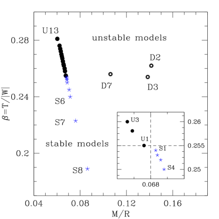
Figure 1: Position on the $(M/R,\beta)$ plane of the stellar models considered. Indicated respectively with stars and filled circles are the stable and unstable models belonging to a sequence of constant rest mass $M_{0}\simeq 1.51\ M_{\odot}$. Open circles refer instead to models which do not belong to the sequence, are also unstable and were first investigated in ref. Shibata et al. (2000). Finally, the inset shows a magnification of the region where the threshold of the instability has been located for the sequence of models investigated.

     

Figure 2: Initial profiles of the rest-mass density $\rho$ (left panel) and of the angular velocity $\Omega$ (right panel) for models S8, S7, S2, U1, U3, U11 and U13. Indicated with a dot-dashed line is the profile for the first unstable model (U1) with $\beta$ = 0.255. Note that this is not the first model having an off-centered maximum of the rest-mass density.

III Initial Data

The initial data for our simulations are computed as stationary equilibrium solutions for axisymmetric and rapidly rotating relativistic stars in polar coordinates Stergioulas and Friedman (1995). In generating these equilibrium models we assumed that the metric describing an axisymmetric and stationary relativistic star has the form

$$\begin{split}ds^{2}=-e^{\mu+\nu}dt^{2}+e^{\mu-\nu}r^{2}\sin^{2}\theta(d\phi-\omega dt)^{2}\\ +e^{2\xi}(dr^{2}+r^{2}d\theta^{2})\end{split}$$ (19)

where $\mu$, $\nu$, $\omega$ and $\xi$ are space-dependent metric functions. Similarly, we assumed the matter to be characterized by a non-uniform angular velocity distribution of the form

$$\Omega_{c}-\Omega=\frac{r_{e}^{2}}{\hat{A}^{2}}\left[\frac{(\Omega-\omega)r^{2}\sin^{2}\theta e^{-2\nu}}{1-(\Omega-\omega)^{2}r^{2}\sin^{2}\theta e^{-2\nu}}\right]\ ,$$ (20)

where $r_{e}$ is the coordinate equatorial stellar radius and the coefficient $\hat{A}$ is a measure of the degree of differential rotation, which we set to $\hat{A}=1$ in analogy with other works in the literature. Once imported onto the Cartesian grid and throughout the evolution, we compute the angular velocity $\Omega$ (and the period $P$) on the $(x,y)$ plane as

$$\Omega=\frac{u^{\phi}}{u^{0}}=\frac{u^{y}\cos\phi-u^{x}\sin\phi}{u^{0}\sqrt{x^{2}+y^{2}}}\,,\qquad P=\frac{2\pi}{\Omega}$$ (21)

and other characteristic quantities of the system, such as the baryonic mass $M_{0}$, the gravitational mass $M$, the angular momentum $J$, the rotational kinetic energy ${T}$ and the gravitational binding energy ${W}$ as

$$M \equiv \int\!d^{3}\!x\,\left(-2T^{0}_{0}+T^{\mu}_{\mu}\right)\alpha\sqrt{\gamma}\quad,$$ (22)

$$M_{0} \equiv \int\!d^{3}\!x\,D\quad,$$ (23)

$${E_{\rm int}} \equiv \int\!d^{3}\!x\,D\epsilon\quad,$$ (24)

$$J \equiv \int\!d^{3}\!x\,T^{0}_{\phi}\alpha\sqrt{\gamma}\quad,$$ (25)

$${T} \equiv \frac{1}{2}\int\!d^{3}\!x\,\Omega T^{0}_{\phi}\alpha\sqrt{\gamma}\quad,$$ (26)

$${W} \equiv {T}+{E_{\rm int}}+M_{0}-M\ ,$$ (27)

where $\alpha\,\sqrt{\gamma}$ is the square root of the four-dimensional metric determinant. We recall that the definitions of quantities such as $J$, ${T}$, ${W}$ and $\beta$ are meaningful only in the case of stationary axisymmetric configurations and should therefore be treated with care once the rotational symmetry is lost.

All the equilibrium models considered here have been calculated using the relativistic polytropic EOS (15) with $K=100$ and $\Gamma=2$ and are members of a sequence having a constant amount of differential rotation with $\hat{A}=1$ and a constant rest mass of $M_{0}\simeq 1.51\ M_{\odot}$ (a part of this sequence has also been considered in refs. Stergioulas et al. (2004) and Dimmelmeier et al. (2006) as models $A8-A10$). These are collected in Fig. 1 in a compactness/instability-parameter plot, where we have indicated with stars the stable models (S1–S8) and with filled circles the unstable ones (U1–U11). In addition, in order to compare with previous results, we have also considered three other models (D2, D3, D7), first investigated in ref. Shibata et al. (2000), which have larger masses and compactnesses. These models are unstable and are marked by circles in Fig. 1. Finally, the inset shows a magnification of the region where the threshold (indicated with a dashed line) of the instability has been located for the members of the sequence.

The main properties of all the considered models are reported in Table 1, while we show in Fig. 2 the profiles of the rest-mass density $\rho$ (left panel) and of the rotational angular velocity $\Omega$ (right panel) for some of the models in the constant–rest-mass sequence. Note that the position of the maximum of the rest-mass density coincides with the center of the star only for models with low $\beta$; for those with a larger $\beta$, the maximum of the rest-mass density resides, instead, on a circle on the equatorial plane. Finally, indicated with a dot-dashed line in Fig. 2 is the profile for the first unstable model (U1) with $\beta=0.255$. Note that this is not the first model having an off-centered maximum of the rest-mass density.

Model		$\rho_{c}$	$r_{p}/r_{e}$	$R_{e}$	$M_{0}$	$M$	$M/R_{e}$	$J$	$P_{a}$	$P_{e}$	$T$	$W$	$\beta$
		$\scriptstyle(10^{-4})$							(ms)	(ms)	$\scriptstyle(10^{-2})$	$\scriptstyle(10^{-2})$
U13		0.5990	0.20010	24.31	1.505	1.462	0.0601	3.747	1.723	3.910	2.183	7.764	0.2812
U12		0.9940	0.24150	23.52	1.508	1.462	0.0622	3.591	1.599	3.654	2.272	8.228	0.2761
U11		1.0920	0.25010	23.31	1.507	1.460	0.0627	3.541	1.572	3.597	2.284	8.327	0.2743
U10		1.1960	0.25860	23.08	1.508	1.460	0.0633	3.496	1.542	3.536	2.302	8.461	0.2721
U9		1.2840	0.26550	22.88	1.508	1.460	0.0638	3.457	1.517	3.486	2.316	8.575	0.2701
U8		1.3470	0.27030	22.73	1.508	1.460	0.0642	3.428	1.500	3.450	2.325	8.659	0.2686
U7		1.4060	0.27470	22.59	1.509	1.460	0.0647	3.402	1.484	3.417	2.334	8.741	0.2671
U6		1.4810	0.28030	22.40	1.508	1.459	0.0651	3.363	1.465	3.377	2.341	8.832	0.2651
U5		1.5530	0.28560	22.22	1.508	1.458	0.0656	3.326	1.446	3.339	2.346	8.920	0.2631
U4		1.5880	0.28810	22.13	1.508	1.458	0.0659	3.310	1.437	3.321	2.351	8.970	0.2621
U3		1.6720	0.29430	21.92	1.506	1.456	0.0664	3.261	1.417	3.279	2.352	9.061	0.2596
U2		1.7230	0.29780	21.78	1.508	1.457	0.0669	3.241	1.404	3.251	2.360	9.146	0.2581
U1		1.8120	0.30500	21.54	1.499	1.448	0.0672	3.164	1.386	3.214	2.336	9.167	0.2549
S1		1.8600	0.30700	21.42	1.512	1.460	0.0682	3.191	1.368	3.180	2.384	9.388	0.2540
S2		1.8850	0.30900	21.35	1.510	1.458	0.0683	3.170	1.364	3.170	2.378	9.396	0.2531
S3		1.9160	0.31100	21.27	1.512	1.459	0.0686	3.160	1.356	3.153	2.385	9.458	0.2522
S4		1.9620	0.31500	21.14	1.504	1.452	0.0687	3.111	1.348	3.137	2.363	9.439	0.2503
S5		2.1280	0.32600	20.70	1.510	1.456	0.0703	3.050	1.308	3.057	2.386	9.736	0.2451
S6		2.2610	0.33600	20.32	1.505	1.449	0.0713	2.965	1.282	3.002	2.369	9.859	0.2403
S7		2.7540	0.37040	19.03	1.506	1.447	0.0760	2.741	1.189	2.812	2.360	10.56	0.2234
S8		3.8150	0.44370	16.70	1.506	1.439	0.0862	2.322	1.048	2.531	2.255	11.96	0.1886
D2		3.1540	0.27500	18.29	2.771	2.587	0.1414	7.620	0.735	2.051	9.256	35.28	0.2624
D3		3.7250	0.30000	17.85	2.640	2.466	0.1382	6.827	0.731	2.026	8.450	33.11	0.2544
D7		2.7960	0.30000	19.56	2.188	2.075	0.1061	5.386	0.959	2.442	5.390	21.06	0.2561

Table 1: Main properties of the stellar models used in the simulations. Starting from the left the different columns report: the central rest-mass density $\rho_{c}$, the ratio between the polar and the equatorial coordinate radii $r_{p}/r_{e}$, the proper equatorial radius $R_{e}$, the rest mass $M_{0}$, the gravitational mass $M$, the compactness $M/R_{e}$, the total angular momentum $J$, the rotational periods at the axis $P_{a}$ and at the equator $P_{e}$, the rotational energy $T$ and the binding energy $W$, and their ratio $\beta$ (instability parameter).

As mentioned in the Introduction, numerical simulations of the dynamical bar-mode instability have traditionally been sped up by introducing sometimes very large initial $m$=2 deformations. The rationale behind this is simple since a seed perturbation has the effect of reducing the time needed for the instability to develop and thus the computational costs. However, as we will discuss in detail in Section VI.3, the introduction of any perturbation (especially when this is not a small one) may lead to spurious effects and erroneous interpretations. Although in almost all of our simulation we have evolved purely equilibrium models and simply used the truncation errors to trigger the instability, we have also considered models which are initially perturbed so as to determine the effect of these perturbations on the evolution of the instability. In these cases, we have modified the equilibrium rest-mass density $\rho_{0}$ with a perturbation of the type

$$\delta\rho_{2}(x,y,z)=\delta_{2}\rho_{0}\frac{x^{2}-y^{2}}{r_{e}^{2}}\ ,$$ (28)

where $\delta_{2}$ is the magnitude of the $m$=2 perturbation (which we usually set to be $\delta_{2}\simeq 0.01-0.3$). This perturbation has then the effect of superimposing on the axially symmetric initial model a bar-mode deformation that is much larger than the (unavoidable) $m$=4-mode perturbation introduced by the Cartesian grid discretization. In addition to a bar-mode deformation and in order to test the effect of a pre-existing $m$=1-mode perturbation we also used in some cases (cf. Section VI.3) an $m$=1-mode density perturbation of the type

$$\delta\rho_{1}(x,y,z)=\delta_{1}\sin\left(\phi+\frac{2\pi\varpi}{r_{e}}\right)\rho_{0}\ ,$$ (29)

with $\delta_{1}=0.01$. Finally, after the addition of a perturbation of the type (28) or (29), we have re-solved the Hamiltonian and momentum constraint equations, in order to enforce that the initial constraint violation is at the truncation-error level.

IV Methodology of the Analysis

A number of different quantities are calculated during the evolution to monitor the dynamics of the instability. Among them is the quadrupole moment of the matter distribution, which we compute in terms of the conserved density $D$ rather than of the rest-mass density $\rho$ or of the $T_{00}$ component of the stress energy momentum tensor

$$I^{jk}=\int\!d^{3}\!x\;D\;x^{j}x^{k}\ .$$ (30)

Of course, the use of $D$ in place of $\rho$ or of $T_{00}$ is arbitrary and all the three expressions have the same Newtonian limit. However, we prefer the form (30) because $D$ is a quantity whose conservation is guaranteed by the form chosen for the hydrodynamics equations (17). The time variation of (30) (or, rather, suitable combinations of its second time derivatives) will then be used in Section VIII to characterize the gravitational-wave emission from the instability.

Once the quadrupole moment distribution is known, the presence of a bar and its size may be usefully quantified in terms of the distortion parameters Saijo et al. (2001b)

$$\eta_{+} =\dfrac{{I}^{xx}-{I}^{yy}}{{I}^{xx}+{I}^{yy}}\quad,$$ (31)

$$\eta_{\times} =\dfrac{2\;{I}^{xy}}{{I}^{xx}+{I}^{yy}}\quad,$$ (32)

$$\eta =\sqrt{\eta_{+}^{2}+\eta_{\times}^{2}}\ .$$ (33)

In addition, the quantity (31) can be conveniently used to quantify both the growth time $\tau_{{}_{\rm B}}$ of the instability and the oscillation frequency $f_{{}_{\rm B}}$ of the unstable bar once the instability is fully developed. In practice, we perform a nonlinear least-square fit of the computed distortion $\eta_{+}(t)$ with the trial function

$$\eta_{+}(t)=\eta_{0}\;e^{t/\tau_{{}_{\rm B}}}\cos(2\pi\,f_{{}_{\rm B}}\,t+\phi_{0})\ .$$ (34)

Note that all quantities (31)–(33) are expressed in terms of the coordinate time $t$ and do not represent therefore invariant measurements at spatial infinity. However, for the simulations reported here, the lengthscale of variation of the lapse function at any given time is always larger than twice the stellar radius at that time, ensuring that the events on the same timeslice are also close in proper time.

Unless stated differently, we generally do not impose any boundary condition enforcing certain symmetries. As a result, during the evolution the compact star is not constrained to be centered at the origin of the coordinate system and, in order to monitor the relative motion of the rest-mass density distribution with respect to the coordinate system, we compute the first momentum of the rest-mass density distribution

$$X_{cm}^{i} = \displaystyle\frac{1}{\widetilde{M}}\;\int\!\!d^{3}\!x\;\rho\;x^{i}\ ,$$ (35)

where $\widetilde{M}\equiv\int\!d^{3}\!x\;\rho$. These quantities are reminiscent of the Newtonian definition of the centre of mass of the star but, because they are not gauge-invariant quantities, they are not expected to be constant during the evolution. However, since in a Newtonian framework a time-variation of one of the $X^{i}_{\rm cm}$ would signal a nonzero momentum in that direction, we monitor these quantities as a measure of the overall accuracy of the simulations. Note also that, since the concept of the centre of mass is well defined in a Newtonian context only, equivalent definitions to (35) could be made in terms of $D$ or of $T_{00}$. We have verified that in our simulations no significant quantitative differences are present among the possible alternative definitions.

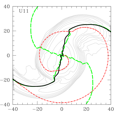
Figure 3: Mode-phases (solid line for the $m$=2 mode, dashed for the $m$=4 mode and dot-dashed for the $m$=1 mode) at different values of $\varpi$ overlapped with isocontours of the rest-mass density for model U11 at 25.7ms.

In addition, as a fundamental tool to describe and understand the nonlinear properties of the development and saturation of the instability, we decompose the rest-mass density into its Fourier modes so that the “power” of the $m$-th mode is defined as

$${P}_{m}\equiv\int\!d^{3}\!x\,\rho\,e^{{\rm i}m\phi}$$ (36)

and the “phase” of the $m$-th mode is defined as

$${\phi}_{m}\equiv\arg({P}_{m})\ .$$ (37)

The phase ${\phi}_{m}$ essentially provides the instantaneous orientation of the $m$-th mode when this has a nonzero power and is expected to have a harmonic time dependence when the corresponding mode has a fully developed mode-component.

An important clarification to make is that, despite their denomination, the Fourier modes (36) do not represent proper eigenmodes of oscillation of the star. While, in fact, the latter are well defined only within a perturbative regime, the former simply represent a tool to quantify, within a fully nonlinear regime, what are the main components of the rest-mass distribution. Stated differently, we do not expect that quasi-normal modes of oscillations are present but in the initial and final stages of the instability, for which a perturbative description is adequate.

Note also that the diagnostic quantities (36) are closely related to the “dipole diagnostic” $D={P}_{1}/M$ and “quadrupole diagnostic” $Q={P}_{2}/M$ of ref. Saijo et al. (2003). For some selected models we have restricted the integration domain in eqs. (36) and (37) to the equatorial [i.e. $(x,y)$] plane and performed an integration in the azimuthal angle $\phi$ only. In this way the corresponding quantities

$${\tilde{P}}_{m}(\varpi) \equiv \int_{z=0}\!\!\!d\phi\;\rho(\varpi\cos(\phi),\varpi\sin(\phi))e^{{\rm i}m\phi}\ ,$$ (38)

$${\tilde{\phi}}_{m}(\varpi) \equiv \arg({\tilde{P}}_{m}(\varpi))\ ,$$ (39)

have an explicit dependence on the cylindrical radial coordinate $\varpi$ only. The quantities (39) have the advantage that they can be used to check the “coherence of the mode” since ${\tilde{\phi}}_{m}(\varpi)$ should be independent of $\varpi$ when the $m$-th mode is a global property of the matter distribution. As an example we show in Fig. 3 the phases for the $m$=1, 2 and $m$=4 modes for model U11 when the bar is still fully developed, just before the bar loses its coherence. Note that the $m$=1 mode shows a spiral-like pattern inside the star, while both ${\tilde{\phi}}_{2}$ and ${\tilde{\phi}}_{4}$ acquire a radial dependence in the outer parts of the star, where the bar deformation is absent. A similar behaviour for the ${\tilde{\phi}}_{m}(\varpi)$ has been observed in all the performed simulations.

V General features of the dynamics

       

      

      

      

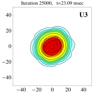
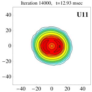
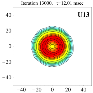
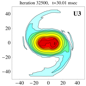
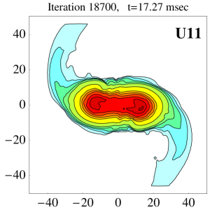
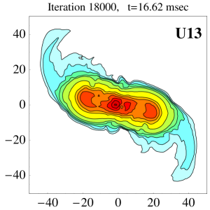
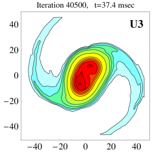
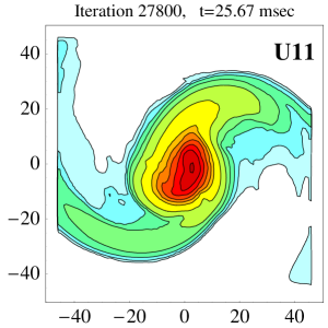
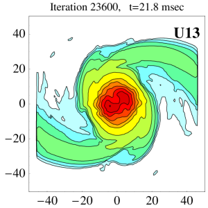
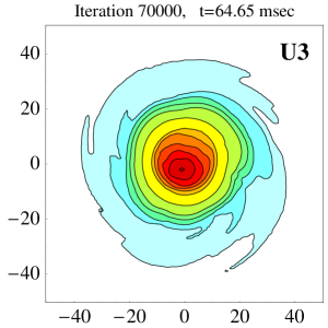
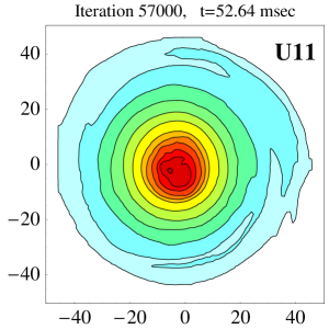
Figure 4: Snapshots of the evolution of models U3, U11 and U13 at various times. The different columns refer to the three models and show isodensity contours for $\rho=0.9,0.8,0.7,0.6,0.5^{-2j}\times\rho_{\rm max}$, where $j=1,\ldots,6$ and $\rho_{\rm max}$ is the maximum value of $\rho$ in each panel. The above models were evolved on a $193\times 193\times 68$ grid with grid coordinate resolution of 0.5 $M_{\odot}$ (0.74km) and imposing equatorial symmetry. The time evolution of some quantities characterising these models is reported in Figs. 5, 6 and 7.

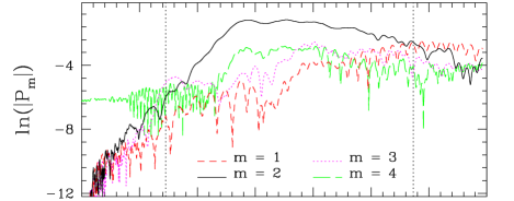
Figure 5: Time evolution of the instability for model U3. The top panel shows the behaviour of the quadrupole distortion parameter $\eta_{+}$ [cf. eq. (33)], the middle panel reports the behaviour of the power in the Fourier modes $m$=1, $2$, $3$ and $4$, while the bottom panel displays the phase of the $m$=2 mode.

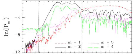
Figure 6: The same as Fig. 5 but for model U11.

V.1 The tests on stable models

Before investigating the nonlinear dynamics of unstable stellar models, we have carried out a systematic investigation of the ability of our code to perform long-term stable and accurate evolutions of stable stellar models. In particular, we have considered the time evolution of two of the differentially rotating models discussed in ref. Stergioulas et al. (2004); Dimmelmeier et al. (2006), namely models S7 and S8, and have followed their dynamics for 24 and 35 axial rotation periods, respectively. In both cases the stellar models remain stable and the density and velocity fluctuations in the stellar interior are smaller than 2% during the whole simulation. This is a rather remarkable result in fully 3D simulations and it is worth stressing that the simulations reported in ref. Font et al. (2002) were not able to go beyond 3 orbital periods for similar values of the grid size and spacing (we recall that in Font et al. (2002) a second-order TVD method with the MC limiter was used in place of the third-order PPM method used here).

In addition, for a more quantitative check of the accuracy of our simulations, we have computed the frequency of the $f$-mode using the normalized power spectrum (Lomb’s method Lomb (1976)) of the coordinate time evolution of the central rest-mass density. The calculated values of 791 Hz for model S8 (A9) and of 674 Hz for model S7 (A10) are in very good agreement, with the values of 809 Hz and 685 Hz reported in ref. Dimmelmeier et al. (2006) and computed using a 2D grid in spherical coordinates but in the conformally flat approximation of General Relativity.

V.2 Common feature of unstable models

In this subsection, we discuss some of the general features of the dynamics of unstable models, postponing to the following sections the discussion of more detailed aspects of the instability. Here we will focus in particular on the dynamics of three representative unstable models, namely U3, U11 and U13, which have been selected so that their increasing values for the $\beta$ parameter cover the whole range of interest. For these simulations, we have used a spatial resolution $\Delta x=0.5\,M_{\odot}$ and a grid of $193\times 193\times 68$ cells and imposed a reflection symmetry with respect the $(x,y)$ plane. As a result, between 80 and 90 gridpoints cover the stars along the $x$ and $y$ axes at time $t=0$. Note that all the simulations reported here make use of a uniform grid with the location of the outer boundary being rather close to the stellar surface; this makes the extraction of gravitational waves difficult and accounts for a very small but nonzero loss of mass and angular momentum (because of matter escaping the computational box).

In Fig. 4 we show some representative snapshots of the rest-mass density at four different times for three different unstable models (one column for each model). In particular, each row refers to one of the four representative stages in which the dynamics of the bar can be divided. These are: (a) exponential growth of the $m$=2 mode and $m$=3 mode (first row); (b) saturation of the instability, development of spiral arms and progressive attenuation of the bar deformation (second row); (c) crossing of $m$=3 mode and $m$=4 mode and consequent attenuation of the bar, emergence of the $m$=1 mode as the dominant one (third row); (d) suppression of the bar deformation and emergence of an almost axisymmetric configuration (fourth row). Note that while these stages are present in all these three models, the coordinate times at which they take place (indicated in the upper part of each panel), as well as the amplitude of the deformation, depend on the parameters defining the initial models, most notably $\beta$ and $M_{0}$.

Understanding the occurrence of these four stages during the onset, development and suppression of the bar deformation represents our effort to go beyond the standard phenomenological discussion of the nonlinear dynamics of the instability often encountered in the literature. An important tool in this discussion will be offered by the time evolution of the Fourier mode-decomposition (36) discussed in Sec. IV. As we will show below, relating the evolution of these quantities to the evolution of the mode phases $\phi_{m}$ and to the changes in the deformation of the star $\eta_{+},\eta_{\times}$ will allow us to provide a consistent description of the four stages of the instability.

We start our discussion by reporting in Figs. 5,  6 and 7 the history of the instability for models U3, U11 and U13. Starting from the upper panels, these figures show: the time evolution of the distortion parameter $\eta_{+}$ (a very similar behaviour can be shown for the other distortion parameter $\eta_{\times}$), the power $P_{m}$ in the first four $m$-modes and the evolution of the phase of the $m$=2 mode. Note that at the beginning of the simulation, as a result of the Cartesian discretization, the $m$=4 mode has the largest power. While this can be reduced by increasing the resolution, the $m$=4 deformation plays no major role in the development of the instability, which is soon dominated by the lower-order modes.

The initial phase of the instability [stage (a) in the previous classification] is clearly characterized by the exponential growth of the $m$=2 mode and $m$=3 mode, the latter one having a smaller growth rate. A first interesting mode coupling takes place when the exponentially growing $m$=3 mode reaches the same power amplitude of the $m$=4 mode, at which point the two modes exchange their dynamics, with the $m$=4 mode growing exponentially and the $m$=3 mode reaching saturation. At approximately the same time, the $m$=1 mode also starts to grow exponentially but with a growth rate which is smaller than that of the other modes. Note that this “mode-amplitude crossing” between the $m$=3 and $m$=4 modes also signals the time when collective phenomena start to be fully visible (note that this mode-amplitude crossing is distinct from the “avoided-crossing” observed when studying mode eigenfrequencies along sequences of stellar models). This is shown with the first vertical dotted line in Figs. 5, 6 and 7, marking the time when the distortion parameter starts being appreciably different from zero (upper panel) and the $m$=2 phase assumes a harmonic time dependence (lower panel). This stage continues until the $m$=2 mode reaches its maximum power and the bar has reached its largest extension. During the following phase [stage (b)] the bar instability has reached a nonlinear saturation, accompanied by the development of spiral arms which are responsible for ejecting a small amount of matter and for a progressive attenuation of the bar extension (see discussion in Sec. VI.1). Furthermore, when the exponentially growing $m$=1 mode reaches the same power amplitude of the $m$=3 mode, the latter, whose growth had slowed down for a while, returns to grow exponentially.

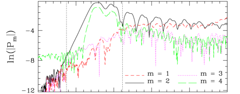
Figure 7: The same as Fig. 5 but for model U13.

The following phase of the instability [stage (c)] sees modes $m$=1, 3 and 4 reach comparable powers and this marks the time when the bar deformation has a sudden decrease. As a result of this crossing among the three modes, only the $m$=1 mode will continue to grow, while the $m$=3 and the $m$=4 modes are progressively damped. Finally, stage (d) starts when the growing $m$=1 mode reaches power amplitudes comparable with those of the $m$=4 mode and the final mode-amplitude crossing takes place. This marks a distinct loss of the bar deformation and the emergence of an almost axisymmetric rapidly rotating star. This is shown with the second vertical dotted line in Figs. 6 and 7, highlighting when the distortion parameter is significantly reduced (upper panel) and the $m$=2-mode phase loses its harmonic time dependence (lower panel). A schematic and qualitative diagram summarizing the evolution of the power in the first four $m$-modes as discussed above is shown in Fig. 8 and can be used as an aid for the interpretation of the quantities computed in Figs. 5,  6 and 7.

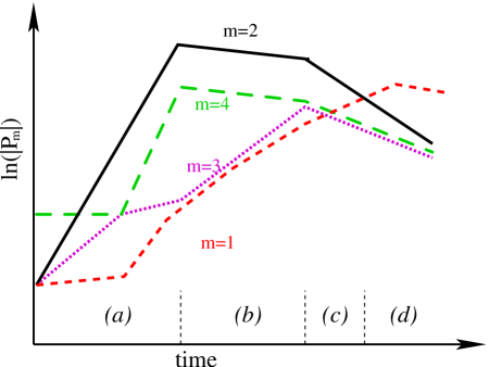
Figure 8: Schematic evolution of the collective modes [Eq. 36] of the rest-mass density $\rho$. In this diagram the instability is distinguished in four representative stages: (a) exponential growth of the $m$=2 mode and $m$=3 mode; (b) saturation of the instability, development of spiral arms and progressive attenuation of the bar deformation; (c) crossing of $m$=3 mode and $m$=4 mode and consequent attenuation of the bar, emergence of the $m$=1 mode as the dominant one; (d) suppression of the bar deformation and emergence of an almost axisymmetric configuration.

We note that the lack of a perturbative study of this process beyond the linear regime leaves the origins of this interaction between modes still unclear. Furthermore, since the growth of the $m$=1 mode is not clearly exponential, especially for slightly overcritical models (cf. Fig. 5 for model U3), we have referred to this process as “mode coupling” rather than considering it as the evidence of an $m$=1 instability. Additional perturbative work in this respect will help clarify this aspect.

The general and common features of the dynamics of the bar-mode instability as deduced from the numerical simulations can be summarized as follows:

• the bar deformation is, in general, not a persistent phenomenon but is suppressed rather rapidly and over a timescale which is of the order of the dynamical one (see also the following Section for an additional discussion on this);

• nonlinear mode couplings take place during the evolution and these allow for the growth of other modes besides the fastest-growing $m$=2 mode;

• the growth of other modes has the overall impact of progressively attenuating the $m$=2 mode and, consequently, the bar deformation, after the instability has saturated;

• for slightly supercritical models (e.g. U3), when the power amplitude of the $m$=1 mode has become comparable with the one in the $m$=2 mode, the bar deformation is suppressed and the star evolves towards an almost axisymmetric configuration;

• for largely supercritical models (e.g. U13), the dynamics of the instability are so violent and the stellar model so far from equilibrium that the strong bar deformation is lost even in the absence of mode-coupling effects (see discussion in Sec. VI.2).

VI Detailed features of the dynamics

In this Section we discuss some detailed aspects of the instability, concentrating our attention on the impact that different values of $\beta$, different boundary conditions, different values of the initial perturbations, different EOSs and different grid resolutions or boundary locations have on the onset and development of the instability. We note that while many of these different prescriptions do not induce qualitative changes, some of them do change the initial relative amplitude of the different modes [and hence the simulation time needed for the instability to develop and the orientation of the bar in the $(x,y)$ plane at a given time during the instability]. In these cases, in order to make meaningful comparisons, we remove these offsets by choosing a suitable shift in time $\Delta t$ and in phase $\Delta\phi$ in such a way that the distortion parameters of the reference model $\eta_{+}^{R}$ and of the new one $\eta_{+}$ have the maximal overlap and are related as

$$\eta_{+}^{(R)}(t)\simeq\alpha\eta_{+}(t+\Delta t)+\beta\eta_{\times}(t+\Delta t)\ ,$$ (40)

where $\alpha=\cos(\Delta\phi)$, $\beta=\sin(\Delta\phi)$.

VI.1 Dependence on $\beta$

The parameter $\beta$ plays a very important role in determining the properties of the nonlinear dynamics of the instability both with regard to the growth rate $\tau_{{}_{\rm B}}$ and to the duration $\tau_{{}_{\rm D}}$ of the saturation stage [stage (b) of Fig. 8]. While the relation between $\beta$ and $\tau_{{}_{\rm B}}$ will be discussed in more detail in Sec. VII, we here concentrate on how the dynamics of the bar, once formed, depend on the degree of overcriticality, i.e. on $\beta-\beta_{c}$, where $\beta_{c}$ marks the separation between stable and unstable models. To illustrate this we will consider two models which are representative of the whole set considered in Table 1 and which have very different values of $\beta$ and consequently very distinct behaviours: the largely overcritical model U13 and the slightly overcritical model U3.

Model U13 has $\beta=0.2812$ and is the most unstable of the studied models, since equilibrium models with larger $\beta$ cannot be produced along the constant–rest-mass sequence chosen here. The clearest feature shown in Fig. 7 for this model is its very rapid growth rate (almost three times larger than the one for U3 as reported in Tab. 2), but also its very effective suppression of the bar deformation. Indeed, the evolution is so rapid that it is very little affected either by initial perturbations or by the imposition of additional symmetries (see next subsections). In this case, in fact, the crossing between the $m$=2 mode and $m$=1 mode is less evident and the bar deformation goes through large variations, as shown by the large oscillations in $P_{2}$ after $t\simeq 16$ ms, during which time the bar seems to disappear and then form again soon after. At about $t\simeq 20$ ms the bar deformation starts disappearing in coincidence with the mode-amplitude crossing. Again as a result of the very violent dynamics, the saturation stage is rather short and the bar is essentially lost after about 8 ms.

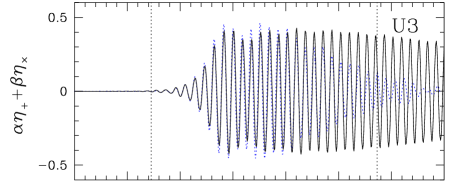
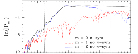
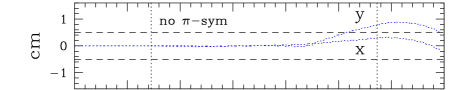
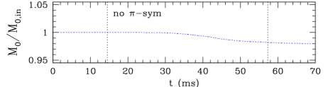
Figure 9: The role of the $\pi$-symmetry on the dynamics for model U3. Shown from the top are the deformation parameter $\eta$, the power in the $m$=2 mode and in the $m$=1 mode (dashed line), the evolution of the position of the “centre of mass” (the horizontal dashed lines mark the edges of the central cell) and that of the rest mass. The dotted and continuous lines refer to simulations without and with $\pi$-symmetry, respectively.

Model U3, on the other hand, has $\beta=0.2596$ and shows dynamics which are in many respects the opposite of the ones discussed for model U13. As shown in Fig. 5, the mode evolution is very smooth and, once formed, the bar persists without significant losses in power. The growth rate is clearly smaller and the stage of saturation is much longer (about 30 ms) and the growth of the $m$=1 mode plays a major role in the damping of the $m$=2 mode. The transition that leads to the disappearance of the bar is smooth and it requires many rotation periods. Differently from model U13, in this case, the properties of the bar dynamics in the first stage are sensitive to the use of perturbations or to the imposition of additional symmetries (see next subsections).

Overall, it is reasonable to expect that the persistence of the bar is strictly related to the degree of overcriticality, with the duration of the saturation $\tau_{{}_{\rm D}}$ tending to the radiation-reaction timescale for a model with $\beta=\beta_{c}$ and to zero for a model with $\beta\gg\beta_{c}$, for which the excess of kinetic rotational energy may well produce a rapid disruption of the star (see Fig. 11). The numerical values for $\tau_{{}_{\rm D}}$ have been estimated through a nonlinear fit to the evolution of $P_{2}$ with 3 separated single exponential functions in the three intervals $[2,t_{a}]$, $[t_{a},t_{b}]$ and $[t_{b},t_{c}]$, where $t_{a}$ and $t_{b}$ are two free parameters and $t_{c}$ marks the end of the simulation. The estimates for $\tau_{{}_{\rm D}}$ reported in Table 2 are still too sparse to be able to delineate its dependence, beyond the evidence that $\tau_{{}_{\rm D}}\propto|\beta-\beta_{c}|^{-n}$, where $n$ is a positive number. Furthermore, the reported values have an error of about $1$ ms, as a result of the used fitting procedure.

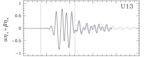
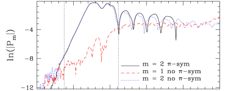
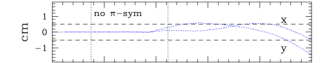
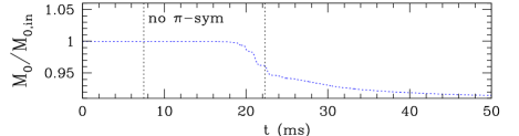
Figure 10: The same as in Fig. 9 but for model U13.

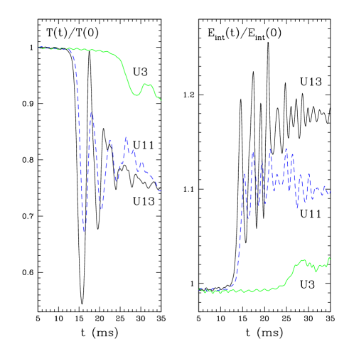
Figure 11: Dynamics of the rotational kinetic energy $T$ [cf. eq. (26)] and of the internal energy ${E}_{\rm int}$ [cf. eq. (24)] for models U3, U11 and U13, when normalized to their initial values.

VI.2 The role of symmetries

As mentioned in the Introduction, the issue of the persistence of the bar deformation has been rather controversial over the years.

While previous calculations carried out in Newtonian physics and in the absence of symmetries have highlighted that the bar deformation can be rapidly suppressed as a result of the growth of an $m$=1-mode deformation Smith et al. (1996), subsequent studies have attributed the growth of the odd mode to inaccurate numerical methods and supported the idea that the bar should be persistent over a radiation-reaction timescale and that the use of suitable symmetry conditions that remove the growth of the odd mode provides a more realistic description of the bar dynamics New et al. (2000). In addition, it has been argued that once an $m$=2-mode perturbation has developed, only couplings with even modes should be expected and that the growth of any odd mode should therefore be considered a spurious numerical artifact.

We believe the above argument not to be valid, except in a linear regime and in the very idealized case in which it is possible to inject exclusively an $m$=2 perturbation. In practice, however, any initial perturbation, either introduced ad hoc or by the truncation error, will excite both even and odd modes and all of these will couple once a nonlinear regime is reached.

Having said this, it is nevertheless important to verify that the growth of the $m$=1 mode detected in our simulations is not a numerical artifact (this is further discussed in Sec. VI.E) and that the argument made about the non-persistence of the bar deformation continues to hold also when boundary conditions with symmetries are introduced. For this reason, we evolved the models discussed in the previous Sections also with the use of the so-called $\pi$-symmetry, ensuring that $f(\varpi,\phi,z)=f(\varpi,\phi+\pi,z)$ for any variable $f(x^{i})$. Clearly, the presence of any odd mode is in this way impossible by construction. We report in Figs. 9-10 the results of the simulations for models U3 and U13 using this symmetry. The first two panels from the top show the deformation parameter $\eta(t)$ and the power in the $m$=2 mode (solid line when the $\pi$-symmetry is enforced and dotted line otherwise) and in the $m$=1 mode (dashed line).

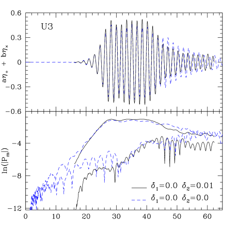
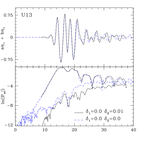
Figure 12: Effect of an initial $m$=2-mode perturbation on the dynamics of the deformation parameter $\eta(t)$ (top sub-panels) and of the modes ${P}_{2}(t)$ and ${P}_{1}(t)$ (bottom sub-panels) for model U3 (left) and U13 (right), respectively. The continuous lines represent the evolution of the perturbed model after a suitable phase and time shifts.

Fig. 9 clearly shows that the bar deformation is essentially persistent in model U3 when the symmetry boundary conditions are applied, its power amplitude being just slowly attenuated, mostly because of the entropy production via the non-isentropic EOS (16) and a possible small contribution due to the use of a tenuous atmosphere outside the star. However, it is important to note that, besides being convergent and stable, the solution without $\pi$-symmetry is also accurate, as well as the one without $\pi$-symmetry. This is shown by the second panel from the bottom in Fig. 9, reporting the evolution of the position of the “centre of mass” as defined in eq. (35), in the absence of $\pi$-symmetry. The two horizontal dashed lines in that panel mark the edges of the central cell and indicate that up to $t\simeq 50$ ms the position of the centre of mass does not leave the central cell of the grid and that the exponential growth of the $m$=1 mode (which becomes significant from $t\simeq 15$ ms) cannot be related to a spurious numerical effect. After $t\simeq 50$ ms the centre of mass starts to move away from the centre of the grid and also in this case the motion is not due to numerical accuracy but rather to the fact that a small amount of matter (about 2% of the initial one) is being lost from the grid as a result of the development of extended spiral arms. This is shown in the lower panel of Fig. 9, which reports the evolution of the rest mass when normalized to the initial value and which clearly shows that the motion of the centre of mass is related to the loss of rest mass through the grid and thus consistent with the conservation of linear momentum. As we will further discuss in Sec. VI.5, the mass loss and the consequent motion of the centre of mass can be reduced considerably when moving the outer boundary to larger positions. As mass leaves the grid, so does angular momentum, with losses that vary according to the model considered and ranging from $\sim 3\%$ for model U3 up to $\sim 20\%$ for the more violent model U13. Note, however, that much smaller angular-momentum losses (i.e. less than 1% for all models) are in general measured before the mass is shed across the computational boundaries; as a result, angular momentum can be conserved to reasonable accuracy by using more distant outer boundaries (this improvement has been tried and a discussion on the changes introduced is presented in Sec. VI.5).

Interestingly, the use of a $\pi$-symmetry does not produce a significant change in the case of model U13. This is true for the dynamics of the bar (cf. the solid and dotted lines in Fig. 10) and also for the values of $\tau_{{}_{\rm B}}$ and $f_{{}_{\rm B}}$. We believe this is because the dynamics of this largely overcritical model are not dominated by the mode coupling, but rather by efficient conversion of rotational kinetic energy into internal energy. As shown in Fig. 11, which reports the time evolution of the internal and rotational kinetic energies when normalized to their initial values, model U13 experiences a dramatic and rapid increase in the internal energy at the expense of the kinetic one. This conversion of energy is the largest among the simulated models and so effective that mode-coupling effects do not have time to develop. This explains why the use of symmetry conditions slightly reduces the attenuation of the bar, but cannot prevent its rapid disappearance.

As a final remark we note that the use of a $\pi$-symmetry produces only small changes in the values of the bar-pattern frequency $f_{{}_{\rm B}}$ or of the growth time $\tau_{{}_{\rm B}}$ when compared with the corresponding values computed in the absence of symmetries (cf. Table 2). This is essentially because these boundary conditions do not alter the dynamics of the stage of exponential growth of the bar. They can therefore be used to reduce the computational costs and pursue the systematic search for the threshold of the instability discussed in Sec. VII.2.

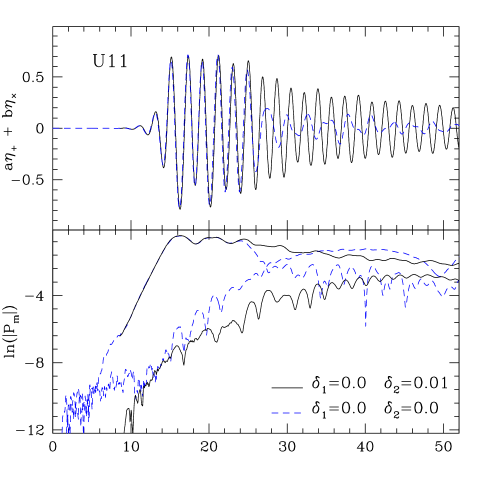
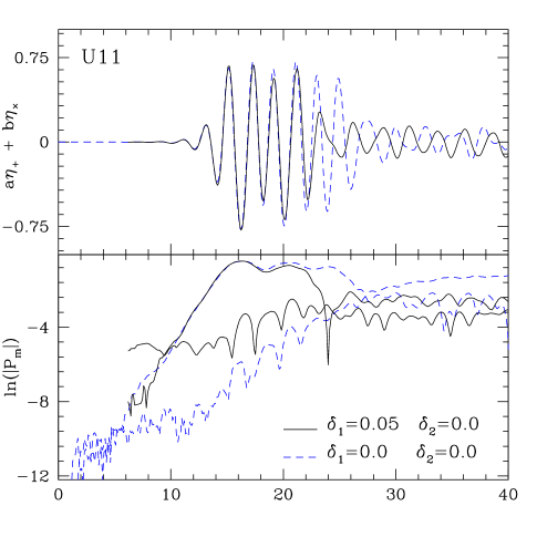
Figure 13: Effect of an initial perturbation on the dynamics of the deformation parameter $\eta$ (top panels) and of the mode powers ${P}_{2}(t)$, ${P}_{1}(t)$ for model U11. The left panel shows the effects of an initial $m$=2-mode perturbation, while the right one those of an $m$=1-mode perturbation.

VI.3 The role of the initial perturbation

Another common feature of previous works on the bar-mode instability has been the introduction of a sizeable $m$=2-mode perturbation of the type shown in eq. (28) with the goal of triggering the instability Shibata et al. (2000); Saijo et al. (2001a, b); Shibata et al. (2002, 2003); Shibata and Sekiguchi (2005). This approach clearly reduces the computational costs but it is fully justified only when the triggered mode is the only unstable one. However, if other unstable modes exist, their development may be altered or even suppressed in the presence of a strong $m$=2-mode perturbation. This is particularly relevant for the analysis carried out in this work, which has pointed out that nonlinear mode couplings may trigger the growth of other modes and significantly modify the dynamics of the instability.

We have therefore considered with care how the introduction of an $m$=2-mode perturbation influences the onset and the development of the instability. More specifically, we have added an $m$=2-mode perturbation of the type shown in eq. (28) with $\delta_{2}=0.01$, solved again the constraint equations and observed that the impact this has on the development of the instability depends on the degree of overcriticality. In particular, for models near the threshold, such as U3, the perturbation does not induce changes in the saturation phase nor in the persistence of the bar, but it does have the effect of slightly altering the first part of the evolution, with an increase in the maximum distortion (which at saturation is $\sim 10\%$ larger) as well as with an increase in the growth rate (the growth time $\tau_{{}_{\rm B}}$ is reduced by $\sim 10~{}\%$); see the left panel of Fig. 12 and Table 2 for a quantitative comparison.

On the other hand, for models that are largely overcritical, such as U13, and in analogy with what discussed in the previous Section for the use of symmetric boundary conditions, the introduction of a perturbation does not have a significant effect and the dynamics are essentially unaltered (see the right panel of Fig. 12). Finally, for models which are overcritical but not close to the threshold, such as U11, the initial perturbation has a much smaller impact on both the growth rate and the maximum distortion (cf. Table 2), but it does increase the duration of the bar. This is due to the fact that the growth of the $m$=1 mode is closely related to the one in the $m$=2 mode and its growth can be delayed and reduced if the latter has initially a non-negligible power. Because of this, the time at which the two modes have comparable power will be different and in particular will be postponed in the perturbed case (see the left panel of Fig. 13). Of course, the converse is also true and modified dynamics for this model are observed also when an $m$=1-mode perturbation of the type shown in eq. (28) is introduced with $\delta_{1}=0.05$. This is summarised in the right panel of Fig. 13, which shows that in this case the perturbation reduces the duration of the saturation stage.

In summary, while the introduction of a seed perturbation (either in the form of an $m$=1 mode or an $m$=2 mode) does not produce significant qualitative changes in the dynamics of the instability, it can result into quantitative changes, most notably in the growth rate, in the maximum distortion and in the persistence of the bar. The persistence of the bar, in particular, is enhanced when an $m$=2-mode perturbation is present. The relevance of these results will need to be evaluated for those astrophysical scenarios in which long-lasting bars were simulated, but which were triggered through the introduction of a perturbation Shibata and Sekiguchi (2005); Shibata et al. (2002).

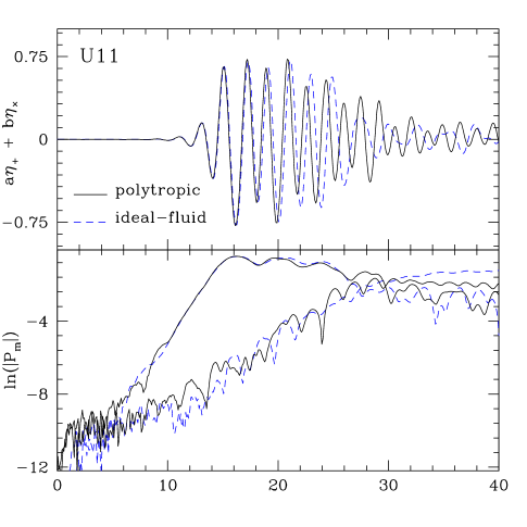
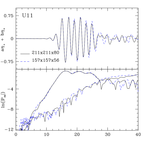
Figure 14: Effects on the evolution of the deformation parameter $\eta$ (top panels) and the modes ${P}_{2}(t)$ and ${P}_{1}(t)$ (bottom panels) of model U11 caused by: (left) the use of the adiabatic polytropic EOS; (right) the use of a larger simulation grid, where the distance of the outer boundary from the center is increased from 48 $M_{\odot}$ to 66 $M_{\odot}$ on the $(x,y)$-plane and from 32 $M_{\odot}$ to 47 $M_{\odot}$ along the $z$ direction.

VI.4 The role of the EOS

Besides nonlinear mode coupling, another process that could in principle limit the persistence of the bar is the formation of shocks (either macroscopical or on smaller scales) that would convert the excess kinetic energy into internal one. In order to assess the importance of this process we have compared the evolution of the relevant unstable models when these are evolved using the non-isentropic EOS (16) and when using the (isentropic) polytropic EOS (15) with $K=100$ and $\Gamma=2$.

The results of this comparison are summarised for model U11 in Fig. 14 and indicate that the non-isentropic changes are indeed very small and that these do not produce any significant variations on the development of the instability and on the growth of the $m$=2 mode. Larger differences are seen in the growth of the $m$=1 mode, but also these are very small and do not produce a qualitative change. Quantitative assessment of the changes produced by a different EOS are reported in Table 2, but these are, overall, comparable with the error bar for the determination of $\tau_{{}_{\rm B}}$ and $f_{{}_{\rm B}}$. Finally, all the considerations made here for model U11 apply also to models U13 and U3, with model U3 being slightly more sensitive to the change in EOS (cf. Table 2). These results indicate therefore that the effects of shock heating are likely to be unimportant at least for the development and evolution of the bar in isolated and old neutron stars.

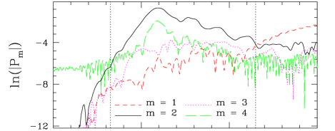
Figure 15: The same as in Fig. 9 but for model D2. In addition, the bottom panel shows the evolution of the phase for the $m=$2 mode.

VI.5 The role of grid spacing and size

We finally report on the influence of the grid spacing and of the grid size on the development of the instability. To assess this we have performed several simulations of the intermediate model U11 differing either in grid resolution or in the location of the outer boundaries. In particular, we have considered grid resolutions $\Delta x/M_{\odot}=0.375$, $\Delta x/M_{\odot}=0.5$ and $\Delta x/M_{\odot}=0.625$ and found the code to be second-order convergent, with the coarsest resolution being just on the limit of the convergence regime (the results with $\Delta x/M_{\odot}=0.75$ are in fact not convergent at the expected rate).

As summarized in Table 2 we have found that the computed values of the instability parameters $\tau_{{}_{\rm B}}$ and $f_{{}_{\rm B}}$ do not vary significantly across the range of resolutions considered, with differences that are at most of about $3\%$. The same Table also contains information on the results obtained when comparing simulations performed with $\Delta x/M_{\odot}=0.625$ but with a larger computational domain, namely going from a computational box, at this resolution, with extents $[157\times 157\times 56]$ to one with extents $[211\times 211\times 80]$. Also in this case the changes in the dynamics are very small (see also the right panel of Fig. 14) and essentially amount to a smaller loss of mass and angular momentum as some of the the matter in the spiral arms is thrown out of the computational grid (see also discussion in Sec. VI.2).

Model	$\Delta x/M_{\odot}$	$\delta_{1}$	$\delta_{2}$	EOS	$\pi$-sym	grid size	$\Delta t$	$t_{1}$	$t_{2}$	${\tau}_{{}_{\rm B}}$	$f_{{}_{\rm B}}$	$\eta$	$\tau_{{}_{\rm D}}$
							(ms)	(ms)	(ms)	(ms)	(Hz)	(max)	(ms)
U3	0.500	$0.0$	$0.0$	polytropic	no	medium	0.76	21	26	2.79	552	0.48	13.8
U3	0.500	$0.0$	$0.0$	ideal fluid	no	medium	0	21	26	2.69	547	0.47	12.9
U3	0.500	$0.0$	$0.01$	ideal fluid	no	medium	-15.94	21	26	2.42	548	0.53	13.0
U3	0.625	$0.0$	$0.0$	ideal fluid	yes	medium	-1.00	21	26	2.82	543	0.43	24.4
U3	0.625	$0.0$	$0.01$	ideal fluid	yes	medium	-16.28	21	26	2.52	547	0.54	24.5
U11	0.500	$0.0$	$0.0$	polytropic	no	medium	5.35	11	14	1.12	497	0.78	8.6
U11	0.500	$0.0$	$0.0$	ideal fluid	no	medium	0	11	14	1.15	494	0.78	9.4
U11	0.500	$0.0$	$0.01$	ideal fluid	no	medium	-8.55	11	14	1.11	494	0.79	9.9
U11	0.375	$0.0$	$0.0$	ideal fluid	no	medium	1.64	11	14	1.11	492	0.79	10.5
U11	0.625	$0.0$	$0.0$	ideal fluid	no	medium	1.79	11	14	1.15	492	0.78	9.0
U11	0.625	$0.0$	$0.0$	ideal fluid	no	large	2.54	11	14	1.15	492	0.78	9.8
U11	0.625	$0.0$	$0.0$	ideal fluid	yes	medium	1.39	11	14	1.12	494	0.77	13.8
U11	0.750	$0.0$	$0.0$	ideal fluid	no	medium	3.79	11	14	1.17	493	0.76	10.8
U11	0.625	$0.05$	$0.0$	ideal fluid	no	medium	6.20	11	14	1.14	495	0.78	6.6
U13	0.500	$0.0$	$0.0$	polytropic	no	medium	1.69	10	13	0.94	457	0.86	5.7
U13	0.500	$0.0$	$0.0$	ideal fluid	no	medium	0	10	13	0.95	454	0.85	6.2
U13	0.500	$0.0$	$0.01$	ideal fluid	no	medium	-8.55	10	13	0.93	454	0.86	6.3
U13	0.625	$0.0$	$0.0$	ideal fluid	yes	medium	-0.16	10	13	0.96	453	0.86	6.5
U13	0.625	$0.0$	$0.01$	ideal fluid	yes	medium	-8.71	10	13	0.94	454	0.86	6.2
D2	0.500	$0.0$	$0.0$	ideal fluid	no	medium	0	9	10.5	0.90	1053	0.59	–
D2	0.500	$0.0$	$0.01$	ideal fluid	no	medium	-6.54	9	10.5	0.78	1052	0.67	–
D2	0.500	$0.0$	$0.04$	ideal fluid	no	medium	-7.57	9	10.5	0.77	1056	0.67	–
D3	0.500	$0.0$	$0.0$	ideal fluid	no	medium	0	9	12	1.54	1086	0.38	–
D7	0.500	$0.0$	$0.0$	ideal fluid	no	medium	0	11	14	1.74	821	0.48	–

Table 2: Main properties of the initial part of the instability for the stellar models used in the simulations. Starting from the left the different columns report: the grid spacing $\Delta x/M_{\odot}$, the amplitudes of the initial perturbations in the $m$=1 and $m$=2 modes $\delta_{1,2}$, the EOS, the symmetry and the grid size used, the time shift $\Delta t$ [cf. eq. (40)], the times $t_{1}$ and $t_{2}$ between which the growth-times $\tau_{{}_{\rm B}}$ and the frequencies $f_{{}_{\rm B}}$ are computed, the maximum value of the distortion parameter $\eta$, and the duration of the bar deformation $\tau_{{}_{\rm D}}$.

VI.6 Comparison with previous studies

To conclude this Section describing the dynamics of the instability, we comment on the important validation of the accuracy of our simulations that comes from a comparison with results previously published in the literature. We have focused, in particular, on the fully general-relativistic simulations published in ref. Shibata et al. (2000) and repeated those relative to the models D2, D3 and D7 discussed there. These stars have instability parameters $\beta$ rather close to the critical one, but are also more massive, with gravitational masses between 2 and 2.6 $M_{\odot}$, and have larger compactnesses (cf. Table 1). The development of the instability for one of these models (D2) is summarised in Fig. 15 and the computed distortion parameter is qualitatively very similar to the one presented in ref. Shibata et al. (2000) and shows that in this compact star the bar [i.e. stage (b) of the classification made in Sec. V.2] is very rapidly attenuated as a result of the development of spiral arms, which are also responsible for a small loss of mass.

The frequencies and the growth times found for these models are also in good agreement with those reported in ref. Shibata et al. (2000), but are not identical; differences are of about 10% (see Table 2 for a close comparison). While there are several differences in the numerical codes used, it should be noted that the simulations reported in ref. Shibata et al. (2000) made use of a substantial perturbation in the $m$=2 mode, with an equivalent $\delta_{2}=0.3$. Although we were not able to reproduce exactly the dynamics of these models (no convergent solution of the constraint equations was found once such a large perturbation was introduced), we recall that large perturbations for models near the threshold do induce a change in the growth rates and effectively reduce the growth times (see discussion in Sec. VI.3).

We believe therefore that the use of a smaller or zero perturbation is the largest source of the difference with the corresponding simulations in ref. Shibata et al. (2000), which we can nevertheless reproduce to very good precision.

VII Determination of the threshold

An important consequence of the high accuracy of our simulations it that it has allowed for a rather precise determination of the stability threshold for the sequence of models considered here. Of course, the determination of the threshold to the third significant figure has little but academic interest, as it is expected not to be universal, but rather to depend (although weakly) on properties such as the degree of differential rotation, the compactness, the EOS, etc.. Nevertheless, this is a useful exercise for at least two different reasons. Firstly, it helps in characterizing the dynamics of slightly supercritical models and, secondly, it allows for a direct comparison with perturbative studies, highlighting when the latter cease to be accurate and how they can be improved.

In what follows we discuss two different methods we have used to this aim. The first one simply selects the initial model with the lowest value of $\beta$ for which an exponential growth in the distortion parameter is seen. The second one, on the other hand, uses the classical Newtonian stability analysis of Maclaurin spheroids for incompressible self-gravitating fluids in equilibrium Chandrasekhar (1969) to extrapolate the position of the threshold also in a fully general-relativistic regime. Interestingly, the results of the two approaches agree to high precision.

VII.1 First method: dynamical evaluation

The approach followed here is straightforward and consists in performing a number of simulations for models with decreasing values of the instability parameter $\beta$ and in determining the critical value $\beta_{c}$ as the smallest one for which an exponential growth of the distortion parameter $\eta$ is observed. More specifically, we have performed a set of 10-ms simulations of models characterized by values of $\beta$ between $\beta=0.24$ and $\beta=0.255$, interval in which the instability was reported to develop Shibata et al. (2000); Saijo et al. (2001a, b). In order to remove a possible contamination by the Cartesian discretization through the power in the $m$=4 mode, all the models had a very small $m$=2-mode perturbation with $\delta_{2}=0.04$, making this the largest mode power initially. Furthermore, since this kind of initial $m$=2-mode perturbation always generates, at least temporarily, a growth of the distortion, we classified as unstable those models for which an exponentially growing bar deformation was observed for the whole simulated 10 ms.

As a result of this set of simulations and of additional refinements of the bracketing interval for the instability, we have concluded that the threshold had to be found between models U2 and S2, although it was not yet obvious whether any or all of these models were unstable. A more precise determination of the nature of these models has therefore required much longer simulations to be performed and that no initial perturbation was introduced. A summary of these long-term simulations is reported in Fig. 16, which shows the evolution for models U1 and S1. The upper panel, in particular, shows the amplitude of the distortion parameter $\eta_{\times}$ for model S1 (continuous line) and U1 (dotted line), respectively, while the lower panel shows the evolution of the power in the $m$=2 mode; indicated with a dashed line is the average value of the $m$=4-mode power for model S1, which does not show an appreciable growth.

While it is evident that model U1 develops an instability over the timescale of the simulation, S1 does not, implying that the threshold for the onset of the dynamical bar-mode instability for the sequence under investigation is $\beta_{c}\simeq 0.255$. We are aware that it may be argued that model S1 is also unstable but with a much smaller growth rate; assessing in practice this would require simulations which are prohibitive with the present computational facilities. However, confidence that the result obtained is correct is also provided by critical-fit analysis, which will be discussed in the following Section.

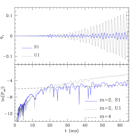
Figure 16: Dynamics of the instability near the threshold. The two panels summarise two long-term evolutions for model S1 (continuous line) and U1 (dotted line) and show the distortion parameter and the power in the $m$=2 and $m$=4 modes.

Model	$\beta$	$\delta_{2}$	$t_{1}$	$t_{2}$	$\eta$	$\tau_{{}_{\rm B}}$	$f_{{}_{\rm B}}$
			(ms)	(ms)	(max)	(ms)	(Hz)
S6	0.240	$0.04$	3	9	0.02	–	$740_{-64}^{+145}$
S5	0.245	$0.04$	3	9	0.02	–	$705_{-64}^{+123}$
S4	0.250	$0.04$	3	9	0.03	–	$656_{-65}^{+71}$
S3	0.252	$0.04$	3	9	0.04	–	$611_{-30}^{+43}$
S2	0.253	$0.04$	3	9	0.05	–	$588_{-12}^{+25}$
S1	0.254	$0.04$	3	9	$*$	9.71	$578_{-21}^{+15}$
U1	0.255	$0.04$	3	9	$*$	5.26	$567_{-4}^{+6}$
S1	0.254	$0.0$	45	63	0.02	–	$599_{-209}^{+209}$
U1	0.255	$0.0$	45	63	$*$	22.1	$588_{-96}^{+56}$

Table 3: The Table reports for some models near the instability threshold: the ratio $\beta$ of the rotational kinetic energy to the gravitational binding energy; the initial $m$=2-mode perturbation $\delta_{2}$; the bounds $t_{1}$ and $t_{2}$ of the considered time interval; the maximum distortion $\eta$; the growth rate $\tau_{{}_{\rm B}}$ and the frequency $f_{{}_{\rm B}}$ of the bar-mode during the initial part of the instability. For these models, $\Delta x/M_{\odot}=0.5$ and $\pi$-symmetry is not used. The growth rate $\tau_{{}_{\rm B}}$ and the frequency $f_{{}_{\rm B}}$ of the bar-mode are obtained making a least-square fit of $\eta_{+}(t)$ (eq.34) between $t_{1}$ and $t_{2}$. The $*$ indicates that $\eta$ did not reach a maximum before the simulation was stopped.

VII.2 Second method: critical fit

The classical Newtonian study of the bar-mode instability is based on the stability analysis of Maclaurin spheroids for an incompressible and self-gravitating fluid in equilibrium Chandrasekhar (1969). We recall that by considering the linearized form of the second-order virial equation, which governs the small oscillations around the equilibrium configuration, it is possible to show that the toroidal $m$=2 perturbations have complex eigenvalues given by (we here use Chandrasekhar’s notation of ref. Chandrasekhar (1969))

$$\sigma=\Omega(e)\pm\sqrt{4B_{11}(e)-\Omega^{2}(e)}\quad,$$ (41)

where $e$ is the eccentricity of the Maclaurin spheroids relative to an incompressible Newtonian star ($e=0$ for a spherical star) and

$$B_{11}\! = \!\frac{3\,e-5\,e^{3}+2\,e^{5}+{\sqrt{1-e^{2}}}\,\left(4\,e^{2}-3\right)\arcsin(e)}{4\,e^{5}}\ ,$$

$$\Omega^{2}\! = \!\frac{6\,\left(e^{2}-1\right)}{e^{2}}+\frac{2\,\left(3-2\,e^{2}\right)\,{\sqrt{1-e^{2}}}\,\arcsin(e)}{e^{3}}\ .$$

As customary in perturbative studies, the real part of the eigenfrequency $\sigma$ represents the characteristic frequency of the small perturbation, while its imaginary part measures the exponential growth time of the $m$=2 mode and is nonzero if $4B_{11}(e)-\Omega^{2}(e)<0$, with the threshold for the instability being marked by the value of the eccentricity for which $4B_{11}(e)-\Omega^{2}(e)=0$. In the case of an incompressible Newtonian star, the eccentricity $e$ and the instability parameter $\beta$ are related as

$$\beta(e)=-1+\frac{3}{2e^{2}}-\frac{3\sqrt{1-e^{2}}}{2e\arcsin(e)}\ .$$ (43)

Equation (41) is most conveniently rewritten in terms of the instability parameter $\beta$ as

$$\sigma=\Omega(\beta)\pm\frac{{\mathrm{i}}}{\tau(\beta)}\quad,$$ (44)

where

$$1/\tau^{2}\equiv-4B_{11}(\beta)+\Omega^{2}(\beta)\ .$$ (45)

Model	$\beta$	$t_{1}$	$t_{2}$	$\eta$	${\tau}_{{}_{\rm B}}$	$f_{{}_{\rm B}}$
		(ms)	(ms)	(max)	(ms)	(Hz)
U2	0.2581	16.9	22.4	0.3734	$3.438_{-1.26}^{+2.39}$	$552_{-30}^{+72}$
U3	0.2595	19.9	24.2	0.4241	$2.678_{-1.23}^{+1.33}$	$544_{-39}^{+86}$
U4	0.2621	15.3	18.3	0.5496	$1.854_{-0.17}^{+0.13}$	$540_{-12}^{+14}$
U5	0.2631	16.2	19.0	0.5788	$1.748_{-0.10}^{+0.12}$	$538_{-13}^{+6}$
U6	0.2651	14.5	17.1	0.6305	$1.574_{-0.04}^{+0.05}$	$528_{-3}^{+6}$
U7	0.2671	14.2	16.4	0.6694	$1.408_{-0.06}^{+0.06}$	$522_{-15}^{+8}$
U8	0.2686	12.2	14.3	0.7027	$1.319_{-0.03}^{+0.06}$	$518_{-6}^{+3}$
U9	0.2701	13.2	15.2	0.7223	$1.269_{-0.04}^{+0.05}$	$512_{-1}^{+3}$
U10	0.2721	13.7	15.6	0.7482	$1.184_{-0.03}^{+0.05}$	$503_{-7}^{+18}$
U11	0.2743	12.9	14.7	0.7749	$1.116_{-0.01}^{+0.04}$	$493_{-11}^{+4}$
U12	0.2761	12.0	13.7	0.7999	$1.066_{-0.03}^{+0.03}$	$486_{-6}^{+5}$
U13	0.2812	11.2	12.7	0.8551	$0.952_{-0.02}^{+0.02}$	$453_{-7}^{+5}$

Table 4: Same quantities as in Table 3, but referring to the models evolved with a grid size of $\Delta x/M_{\odot}=0.625$, with $\pi$-symmetry and no perturbation. The growth rate $\tau_{{}_{\rm B}}$ and the frequency $f_{{}_{\rm B}}$ of the bar-mode are obtained making a least-square fit of $\eta_{+}(t)$ (eq.34) between $t_{1}$ and $t_{2}$. The interval $[t_{1},t_{2}]$ is here determined, differently from the previous tables, as the one in which $\eta(t)$ is between 5% and the 25% of its first maximum. These models were used to determine the threshold.

With this in mind it is natural to ask how accurate is the Newtonian description of an incompressible Maclaurin spheroid in describing the nonlinear dynamics of a relativistic differentially rotating star. Of course also in full General Relativity the transition between stable and dynamical unstable bar-modes will be described by a change from real to imaginary of the $m$=2-mode eigenfrequency and it is therefore reasonable to expect that the frequencies and the growth times depend on $\beta$ as

$$\frac{\Omega(\beta)}{2\pi} \approx f_{c}+f^{(1)}_{c}(\beta-\beta_{c})+f^{(2)}_{c}(\beta-\beta_{c})^{2}\ ,$$ (46)

$$\frac{1}{\tau^{2}} \approx \frac{1}{k^{2}}(\beta-\beta_{c})\quad.$$ (47)

Using this ansatz, we have performed a series of simulations for models U2–U13 using a $\pi$-symmetry and a grid resolution of $\Delta x/M_{\odot}=0.625$, through which we have computed the values for $f_{{}_{\rm B}}$ and $\tau_{{}_{\rm B}}$ by means of a nonlinear least-square fit to the trial form of eq. (34). Making use of these results, which are collected in Table 4, we have then again used a least-square fit of the values $f_{{}_{\rm B}}$ and $\tau_{{}_{\rm B}}$ to the expected $\beta$ dependence of eqs. (46) and (47) to obtain the unknown coefficients $f_{c},f^{(1)}_{c},f^{(2)}_{c}$, $k$ and $\beta_{c}$:

$$f_{c} =554\,\mbox{Hz}\ , f^{(1)}_{c} =-1668\,\mbox{Hz}\ , f^{(2)}_{c} =-85635\,\mbox{Hz}\ ,$$

$$\beta_{c} =0.2554\ , k =0.153\ \mbox{ms}\ .$$

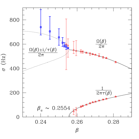
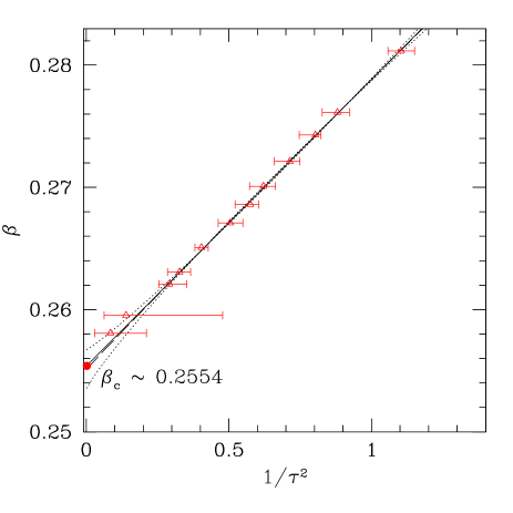
Figure 17: Left panel: critical diagram as constructed with the frequencies and growth times relative to the unperturbed models of Table 4 (triangles) and to the perturbed models of Table 3 (squares). The continuous lines represent the two fitted curves for $\Omega(\beta)$ and $\tau(\beta)$, while the dotted line the corresponding extrapolations below the threshold. Right panel: same data as in the left panel but magnified around the critical threshold and expressed in terms of $1/\tau^{2}$ to highlight the very good fit.

In the left panel of Fig. 17 we summarize the results of this fit for the models U2–U13 and show the corresponding error bars. In particular, we denote with triangles the unperturbed models reported in Table 4, while with squares the perturbed models in Table 3. In addition, the continuous lines represent the two fitted curves for $\Omega(\beta)$ and $\tau(\beta)$, while the dotted line refers to the corresponding extrapolations below the threshold. We note that the error bars in Fig. 17 are computed in different ways for the growth rates and the frequencies. In the first case they are computed as the difference between the minimum and maximum values of $d\log(\eta(t))/dt$ in the time intervals between $t_{1}$ and $t_{2}$ reported in Table 4. In the second case, instead, the error bars are determined using the minimum and maximum values over the time intervals between $t_{1}$ and $t_{2}$ reported in Tables 3 and 4 of the pattern speeds extracted from the collective phase $\phi_{2}(t)$ of eq. (37).

A number of comments are worth making. Firstly, it is clear that the Newtonian description of the instability in terms of incompressible Maclaurin spheroids is surprisingly accurate also in full General Relativity and for differentially rotating stars. It is especially so for models which are far from the instability threshold, for which the error bars are very small and below 5%. Secondly, as the models approach the critical threshold from above (i.e, unstable models), the growth times become increasingly large and the numerical errors increasingly more important for the resolutions we could use. Yet, even in this regime the perturbative predictions are accurate to better than 15%. Finally, as the models approach the critical threshold from below (i.e, stable models), the frequencies of the oscillations triggered by the use of an initial perturbation are similar to the spin frequencies, making the determination of the eigenfrequencies increasingly difficult and hence inaccurate (cf. the large error bars for models denoted by squares in the left panel of Fig. 17).

Finally we note that the independent determination of the threshold for the instability provided by the fit to eq. (47) (i.e. $\beta_{c}=0.2554$) is in surprisingly good agreement with the one obtained in the previous Section, i.e. $\beta_{c}\simeq 0.255$, confirming the accuracy of the dynamical determination and suggesting that model S1 is indeed stable. The very good fit of the data is shown in the right panel of Fig. 17, which reports the same data as in the left panel but magnified around the critical threshold and shown in terms of $1/\tau^{2}$ to highlight the functional dependence as expressed by eq. (47).

VIII Gravitational-Wave emission and detection of the unstable models

One of the goals of this study is to assess whether a dynamical bar-mode instability triggered in a neutron-star model could be a good source of gravitational radiation for the detectors presently collecting data (LIGO, GEO), in the final stages of construction (Virgo) or in the planning phase (Dual) Bonaldi et al. (2003). The use of uniform grids in these calculations has prevented us from placing the outer boundaries at distances sufficiently large to allow a gauge-invariant extraction of the gravitational waves Abrahams et al. (1998); Rupright et al. (1998); Rezzolla et al. (1999). However, a reasonable measure of the amplitude of the expected gravitational radiation and of the consequent SNR is still possible by making use of the standard quadrupole formula Misner et al. (1973). A number of comparative tests have been carried out among the various ways in which the gravitational-wave amplitudes can be estimated (see, for instance, refs. Tanaka et al. (1993); Shibata and Sekiguchi (2005); Nagar et al. (2005)) and we expect the error in this case to be ${\cal O}(M/R)$ Shibata and Sekiguchi (2003) and thus of a few percent only.

In this approximation, the observed waveform and amplitude for the two polarizations measured by an observer situated at infinity along the $z$-axis are

$$\begin{split}h_{+}&=\dfrac{\ddot{I}^{xx}(t^{\prime})-\ddot{I}^{yy}(t^{\prime})}{r}\ ,\\ h_{\times}&=2\;\dfrac{\ddot{I}^{xy}(t^{\prime})}{r}\ ,\end{split}$$ (48)

where $t^{\prime}=t-r$ is the retarded time. The total gravitational wave luminosity is then given by

$$\dot{E}=\dfrac{1}{5}\big{\langle}\dddot{I}^{\,ij}\dddot{I}_{ij}\big{\rangle}\ ,$$ (49)

while the angular momentum loss is

$$\dot{J_{i}}=\dfrac{2}{5}\big{\langle}\epsilon_{ijk}\ddot{I}^{jl}\dddot{I}_{lk}\big{\rangle}\ .$$ (50)

We note that the definition of the quadrupole tensor is not unique as $\rho$ and $D$ coincide in a Newtonian approximation and either of them could be used. Following ref. Shibata et al. (2000), we adopt the definition expressed in eq. (30), as this allows us to exploit the conservation equation for $D$ to perform analytically the first time derivative of the quadrupole tensor and obtain that

$$\dot{I}^{ij}=\int d^{3}\!x\;D\;\left[x^{i}(\alpha v^{j}+\beta^{j})+x^{j}(\alpha v^{i}+\beta^{i})\right]\ ,$$ (51)

from which we compute the second $\ddot{I}^{ij}$ and third $\dddot{I}^{\,ij}$ time-derivatives using first-order finite differencing. This approach not only is simpler, but it is indeed the only possible one, since our second-order–accurate scheme would not allow for an accurate direct calculation of $\dddot{I}^{\,ij}$ (see discussion in Appendix A of ref. Rezzolla et al. (1999)).

Figure 18: Gravitational-wave signals along the $z$-axis for the “cross” polarization as computed in the Newtonian quadrupole approximation for models U3, U11, U13 and D2.

In Fig. 18 the we show the waveforms for the “cross” polarization computed in this way, as measured along the $z$-axis for models U3, U11, U13 and D2 (We recall that the “cross” and “plus” waveforms for a stationary and rotating bar differ only by a phase, since the emission is circularly polarized). Clearly, the gravitational-wave signal mimics (modulo a factor of 2 in the frequency) the dynamical behaviour of the bar deformation, with signals that are longer for models near the stability threshold (i.e. model U3), and with amplitudes which increase for the more compact model D2.

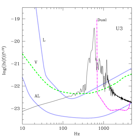
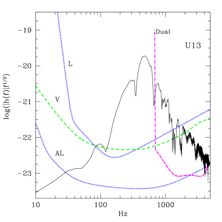
Figure 19: Comparison between $|\tilde{h}(f)|f^{1/2}$ for models U3 and U13 at 10kpc and the square-root of the power spectrum of the noise of Virgo (dashed line), LIGO (dotted line), Advanced LIGO (dotted-line) and the planned resonant detector Dual (dot-dashed line). Note the significant difference in the power spectrum of the two signals, with the one relative to model U3 having a larger and narrower peak at about 600 Hz, produced by the more persistent bar deformation.

Model	$\Delta M/M$	$\Delta J/J$	$h_{\rm rss}$	$SNR$	$SNR$	$SNR$	$SNR$
	$\scriptstyle(10^{-5})$	$\scriptstyle(10^{-3})$	$\scriptstyle(10^{-20})$	V	L	AL	Dual
U3	$7.75$	$3.82$	$1.39$	117	82.5	1590	19
U11	$9.48$	$4.84$	$1.74$	155	119	2040	23
U13	$6.23$	$3.18$	$1.51$	138	114	1780	30
D2	$52.6$	$10.2$	$2.50$	136	79.8	2270	892

Table 5: List of the representative gravitational-wave quantities computed in the Newtonian quadrupole approximation for models U3, U11, U13 and D2. From the left the different columns report: the fractional amounts of the energy and angular momentum carried by the gravitational radiation ($\Delta M/M$ and $\Delta J/J$, respectively), the root-sum-square of $h_{+}$ for a source at 10 kpc, and the SNRs for Virgo, LIGO, Advanced LIGO and Dual.

A convenient measure of the strength of the signal can be given in terms of the root-sum-square amplitude of, say, the plus polarization

$$h_{\rm rss}=\left[\int_{-\infty}^{+\infty}\!\!\!\!dt\,h_{+}^{2}(t)\right]^{1/2}\ ,$$ (52)

since $h_{\rm rss}$ has the same units as the strain-noise amplitude of the detectors and it is therefore possible to obtain a rough estimate of the SNR simply dividing it by the strain-noise amplitude at the frequency where the signal is the strongest. In Table 5 we report the values of $h_{\rm rss}$ for a signal coming from a source at 10 kpc, together with the SNR computed assuming the optimal use of match-filtering techniques and given by

$$\frac{S}{N}=2\sqrt{\int_{0}^{+\infty}\!\!d\log f\;\frac{|\tilde{h}_{+}(f)|^{2}f}{S_{n}(f)}}\quad,$$ (53)

where $\tilde{h}_{+}(f)$ is the Fourier transform of $h_{+}(t)$ and $S_{n}(f)$ is the designed sensitivity of either Virgo (V), LIGO (L), Advanced LIGO (AL) or of the planned resonant detector Dual. Of course, the SNR is inversely proportional to the distance from the source and the values reported in Table 5 indicate that, while an instability developing in a rapidly rotating star in our Galaxy would yield an extremely strong signal, the SNR is still expected to be ${\cal O}(1)$ also for a source as far as about 10 Mpc if measured by Advanced LIGO. A different representation of the results summarised in Table 5 is offered in Fig. 19, which shows a spectral comparison between the designed sensitivity $h_{rms}(f)\equiv\sqrt{S_{n}(f)}$ of Virgo, LIGO and Advanced LIGO and the power spectrum $|\tilde{h}_{+}(f)|f^{\frac{1}{2}}$ of the expected signals for models U3 and U13.

It is interesting to note the significant differences in the power spectrum of the two signals, with the one relative to model U3 having a larger and narrower peak as a result of a more persistent bar. Yet, the SNR for model U3 is significantly smaller than the one for both models U11 and U13 and a number of different factors are behind this somewhat surprising result. Firstly, while the bar is indeed more persistent for U3, the amplitude of the bar distortion is larger for models U11 and U13, thus larger is the corresponding gravitational-wave signal. Secondly, the frequency of the power-spectrum maximum is smaller for models U11 and U13 and thus better fitting the sensitivities of the detectors. Finally, the idealised assumption that match-filtering techniques can be used at all frequencies implies that all of the power spectrum contributes to the final SNR and the large wings of the spectra of models U11 and U13 can significantly increase the SNR. Indeed, when evaluating eq. (53) in a narrow window of 100 Hz around the peak, the SNR of the different models is comparable.

Of course, a strong SNR is just a necessary condition for the detection and the possibility of measuring the gravitational-wave signal from this process will depend significantly on its event rate, which is still largely uncertain. In the case in which the instability develops in a hot protoneutron star resulting from the collapse of a stellar core, the event rate is strictly related to the supernova event rate, which is of 1 or 2 supernova per century per galaxy. About 60% of the remnants of the explosion should be neutron stars, but the requirement of rapid rotation in the progenitor makes the event rate of dynamical instabilities considerably lower Kokkotas and Stergioulas (2005), although such prospect may be more optimistic after recent studies Ott et al. (2006). On the other hand, in case the bar is produced as a result of a binary merger of neutron stars, the most optimistic scenarios suggest that such mergers may occur approximately once per year within a distance of about 50 Mpc Kalogera et al. (2004). Finally, the event rate of the classical scenario in which the instability is triggered in an old neutron star spun up by accretion in a binary system, still remains difficult to quantify.

IX Conclusions

We have presented accurate simulations of the dynamical bar-mode instability in full General Relativity. An important motivation behind this work is the need to go beyond the standard phenomenological discussion of the instability and to find answers to important open questions about its nonlinear dynamics. Among such open problems there are, for instance, the determination of the role of the initial perturbation or of the symmetry conditions, or the influence on the dynamics of the value of the parameter $\beta$, or, most importantly, the determination of the timescale of the persistence of the bar deformation once this is fully developed. Clearly, this latter question is a very pressing one in gravitational-wave astronomy, as it bears important consequences on the detectability of the whole process.

In order to provide answers to these questions we have explored the onset and development of the instability for a large number of initial stellar models. These have been calculated as stationary equilibrium solutions for axisymmetric and rapidly rotating relativistic stars in polar coordinates. More specifically, the evolved models represent relativistic polytropes with adiabatic index $\Gamma=2$ and are members of a sequence having a constant amount of differential rotation with $\hat{A}=1$ and a constant rest mass of $M_{0}\simeq 1.51\ M_{\odot}$.

The simulations have been carried out with the general-relativistic hydrodynamics code Whisky, in which the hydrodynamics equations are written as finite differences on a Cartesian grid and solved using HRSC schemes Baiotti et al. (2003, 2005). The Einstein, equations, on the other hand, have been solved within the conformal traceless formulation implemented within the Cactus computational toolkit Cac .

The main results of our analysis can be summarised as follows: i) An initial $m$=1 or $m$=2-mode perturbation can play a role in determining the duration of the bar-mode deformation, but not the growth time of the instability; the only exception to this is represented by models near the threshold; ii) For moderately overcritical models the use of a $\pi$-symmetry can radically change the dynamics and extend considerably the persistence of the bar; this ceases to be true for largely overcritical models; iii) The persistence of the bar is strongly dependent on the degree of overcriticality and is generically of the order of the dynamical timescale; iv) Generic nonlinear mode-coupling effects (especially between the $m$=1 and the $m$=2 mode) appear during the development of the instability and these can severely limit the persistence of the bar deformation and eventually suppress the bar deformation; v) The dynamics of largely overcritical models (i.e. with $\beta\gg\beta_{c}$) are fully determined by the excess of rotational energy and the bar deformation is very rapidly suppressed through the conversion of kinetic energy into internal one. Interestingly, a similar dynamics for the odd and even modes has been observed also in the case of the low-$\beta$ instability in recent Newtonian simulations Ou and Tohline (2006). In this case, however, the growth rate of the $m$=1 mode is much smaller and hence the persistence of the bar longer.

Finally, we have considered whether the classical Newtonian stability analysis of Maclaurin spheroids for incompressible self-gravitating fluids is accurate also for differentially rotating and relativistic stars. Overall, we have found the perturbative predictions to be surprisingly accurate in determining the threshold for the instability as well as the complex eigenfrequencies for the unstable models.

While the features of the bar-mode instability discussed here are expected to be rather generic, they have been deduced from the analysis of a small region of the space of parameters. Work is now in progress to extend the present analysis by considering stellar models with different and larger compactnesses and that are regulated by more realistic EOSs.

- (1)
- Chandrasekhar (1969) S. Chandrasekhar, Ellipsoidal Figures of Equilibrium (Yale Univ. Press, New Haven, 1969).
- Shapiro and Teukolsky (1983) S. L. Shapiro and S. A. Teukolsky, Black Holes, White Dwarfs, and Neutron Stars (John Wiley & Sons, New York, 1983).
- Tohline et al. (1985) J. E. Tohline, R. H. Durisen, and M. McCollough, Astrophys. J. 298, 220 (1985).
- Durisen et al. (1986) R. H. Durisen, R. A. Gingold, J. E. Tohline, and A. P. Boss, Astrophys. J. 305, 281 (1986).
- Brown (2000) J. D. Brown, Phys. Rev. D 62, 084024 (2000).
- Houser et al. (1994) J. L. Houser, J. M. Centrella, and S. C. Smith, Phys. Rev. Lett. 72, 1314 (1994).
- Houser and Centrella (1996) J. L. Houser and J. M. Centrella, Phys. Rev. 54, 7278 (1996).
- Smith et al. (1996) S. C. Smith, J. L. Houser, and J. M. Centrella, Astrophys. J. 458, 236 (1996).
- New et al. (2000) K. C. B. New, J. M. Centrella, and J. E. Tohline, Phy. Rev. D 62, 064019 (2000).
- New and Shapiro (2001) K. C. B. New and S. L. Shapiro, Astrophys. J. 548, 439 (2001).
- Liu (2002) Y. T. Liu, Phys. Rev. D 65, 124003 (2002).
- Pickett et al. (1996) B. K. Pickett, R. H. Durisen, and G. A. Davis, Astrophys. J. 458, 714 (1996).
- Tohline and Hachisu (1990) J. E. Tohline and I. Hachisu, Astrophys. J. 361, 394 (1990).
- Karino and Eriguchi (2003) S. Karino and Y. Eriguchi, Astrophys. J. 592, 1119 (2003).
- Shibata et al. (2002) M. Shibata, S. Karino, and Y. Eriguchi, Mon. Not. R. Astron. Soc. 334, L27 (2002).
- Shibata et al. (2003) M. Shibata, S. Karino, and Y. Eriguchi, Mon. Not. R. Astron. Soc. 342, 619 (2003).
- Saijo et al. (2003) M. Saijo, T. W. Baumgarte, and S. Shapiro, Astrophys. J. 595, 352 (2003).
- Ott et al. (2005) C. D. Ott, S. Ou, J. E. Tohline, and A. Burrows, Astrophys. J. 625, L119 (2005).
- Shibata et al. (2000) M. Shibata, T. W. Baumgarte, and S. L. Shapiro, Astrophys. J. 542, 453 (2000).
- Saijo et al. (2001a) M. Saijo, M. Shibata, T. W. Baumgarte, and S. L. Shapiro, in 20th Texas Symposium on relativistic astrophysics, edited by J. C. Wheeler and H. Martel, AIP Conf. Proc. No. 586 (AIP, New York, 2001), p. 766.
- Saijo et al. (2001b) M. Saijo, M. Shibata, T. W. Baumgarte, and S. L. Shapiro, Astrophys. J. 548, 919 (2001b).
- Dessart et al. (2006) L. Dessart, A. Burrows, C. D. Ott, E. Livne, S.-C. Yoon, and N. Langer, Astrophys. J. 644, 1063 (2006).
- Shibata and Sekiguchi (2005) M. Shibata and Y.I. Sekiguchi, Phys. Rev. D 71, 024014 (2005).
- Saijo (2005) M. Saijo, Phys. Rev. D 71, 104038 (2005).
- Baiotti et al. (2003) L. Baiotti, I. Hawke, P. Montero, and L. Rezzolla, in Computational Astrophysics in Italy: Methods and Tools, edited by R. Capuzzo-Dolcetta, Memorie della Societá Astronomica Italiana Supplement (SAIT, Trieste, 2003), vol. 1, p. 327.
- Baiotti et al. (2005) L. Baiotti, I. Hawke, P. J. Montero, F. Löffler, L. Rezzolla, N. Stergioulas, J. A. Font, and E. Seidel, Phys. Rev. D 71, 024035 (2005).
- Richtmyer and Morton (1967) R. D. Richtmyer and K. Morton, Difference Methods for Initial Value Problems (Interscience Publishers, New York, 1967).
- York (1979) J. W. York, Jr., in Sources of Gravitational Radiation, edited by L. L. Smarr (Cambridge University Press, Cambridge, UK, 1979), p. 83.
- Nakamura et al. (1987) T. Nakamura, K. Oohara, and Y. Kojima, Prog. Theor. Phys. Suppl. 90, 1 (1987).
- (31) www.cactuscode.org.
- Bona et al. (1995) C. Bona, J. Massó, E. Seidel, and J. Stela, Phys. Rev. Lett. 75, 600 (1995).
- Alcubierre (1997) M. Alcubierre, Phys. Rev. D 55, 5981 (1997).
- Alcubierre and Massó (1998) M. Alcubierre and J. Massó, Phys. Rev. D 57, R4511 (1998).
- Alcubierre et al. (2001) M. Alcubierre, B. Brügmann, D. Pollney, E. Seidel, and R. Takahashi, Phys. Rev. D 64, 061501(R) (2001).
- Smarr and York (1978) L. Smarr and J.W. York, Phys. Rev. D 17, 2529 (1978).
- Font (2003) J. A. Font, Living Rev. Relativity 6, 4 (2003).
- Stergioulas and Friedman (1995) N. Stergioulas and J. L. Friedman, Astrophys. J. 444, 306 (1995).
- Stergioulas et al. (2004) N. Stergioulas, T. A. Apostolatos, and J. A. Font, Mon. Not. R. Astron. Soc. 352, 1089 (2004).
- Dimmelmeier et al. (2006) H. Dimmelmeier, N. Stergioulas, and J. A. Font, Mon. Not. R. Astron. Soc. 368, 1609 (2006).
- Font et al. (2002) J. A. Font, T. Goodale, S. Iyer, M. Miller, L. Rezzolla, E. Seidel, N. Stergioulas, W. M. Suen, and M. Tobias, Phys. Rev. D 65, 084024 (2002).
- Lomb (1976) N. R. Lomb, Astr. Space Sci. 39, 447 (1976).
- Bonaldi et al. (2003) M. Bonaldi, M. Cerdonio, L. Conti, M. Pinard, G.A. Prodi, L. Taffarello, and J.P. Zendri, Phys. Rev. D 68, 102004 (2003).
- Abrahams et al. (1998) A. M. Abrahams, L. Rezzolla, M. E. Rupright, A. Anderson, P. Anninos, T. W. Baumgarte, N. T. Bishop, S. R. Brandt, J. C. Browne, K. Camarda, et al., Phys. Rev. Lett. 80, 1812 (1998).
- Rupright et al. (1998) M. E. Rupright, A. M. Abrahams, and L. Rezzolla, Phys. Rev. D 58, 044005 (1998).
- Rezzolla et al. (1999) L. Rezzolla, A. M. Abrahams, R. A. Matzner, M.E. Rupright, and S.L. Shapiro, Phys. Rev. D 59, 064001 (1999).
- Misner et al. (1973) C. W. Misner, K. S. Thorne, and J. A. Wheeler, Gravitation (W. H. Freeman, San Francisco, 1973).
- Tanaka et al. (1993) T. Tanaka, M. Shibata, M. Sasaki, H. Tagoshi, and T. Nakamura, Prog. Theor. Phys. 90, 65 (1993).
- Nagar et al. (2005) A. Nagar, J. A. Font, O. Zanotti, and R. De Pietri, Phys. Rev. D 72, 024007 (2005).
- Shibata and Sekiguchi (2003) M. Shibata and Y.I. Sekiguchi, Phys. Rev. D 68, 104020 (2003).
- Kokkotas and Stergioulas (2005) K. D. Kokkotas and N. Stergioulas, in Proceedings of the 5th International Workshop ”New Worlds in Astroparticle Physics” (2005), eprint gr-qc/0506083.
- Ott et al. (2006) C. D. Ott, H. Dimmelmeier, A. Marek, J. H. T., I. Hawke, B. Zink, and E. Schnetter (2006), eprint astro-ph/0609819.
- Kalogera et al. (2004) V. Kalogera et al., Astrophys. J. 601, L179 (2004).
- Ou and Tohline (2006) S. Ou and J. E. Tohline, Astrophys. J. 651, 1068 (2006).