Polarization of Quasars: Resonant Line Scattering in the Broad Absorption Line Region

Abstract

Recent works showed that the absorbing material in broad absorption line (BAL) quasars is optically thick to major resonant absorption lines. This material may contribute significantly to the polarization in the absorption lines. In this paper, we present a detailed study of the resonant line scattering process using Monte-Carlo method to constrain the optical depth, the geometry and the kinematics of BAL Region (BALR). By comparing our results with observed polarized spectra of BAL quasars, we find: (1) Resonant scattering can produce polarization up to 9% at the absorption trough for doublet transitions and up to 20% for singlet transitions in radially accelerated flows. To explain the large polarization degree in the CIV, NV absorption line troughs detected in a small fraction of BAL QSOs, a nonmonotonic velocity distribution along the line of sight or/and additional contribution from the electron scattering region is required. (2) The rotation of the flow can lead to the rotation of the polarization position angle (PA) in the line trough. Large extending angle of BALR is required to produce the observed large PA rotation in a few BAL QSOs. (3) A large extending angle of BALR is required to explain a sub-trough in the polarized flux that was observed in a number of BAL QSOs. (4) The resonant-scattering can contribute a significant part of NV emission line in some QSOs, and may give rise to anomalous strong NV lines in these quasars. (5) The polarized flux and PA rotation produced by the resonant scattering in non-BAL is uniquely asymmetric, which may be used to test the presence of BALR in non-BAL QSOs.

1 Introduction

Blue-shifted, broad absorption lines (BAL) are observed in the ultraviolet spectra of about 10-20% luminous quasars. These lines are formed in partially ionized outflows with velocities up to 0.1 c. The outflow is likely driven by intensive radiation of the quasar probably along the equatorial directions to the extension at least larger than the broad emission line region, and is likely several 10 parsecs. Disk wind and material evaporating from the putative dust torus are two plausible scenarios for the origin of the gas. It is usually believed that BAL region exists in every quasar, but only covers a small fraction of quasar sky (Weymann et al. 1991; Reichard et al. 2003; Green et al. 2001; Hamann, Korista & Morris 1993, hereafter HKM93). The outflow may carry a significant fraction of power released by the accretion process and momentum into the host galaxy of the quasar, so that it will influence the subsequent evolution of the galaxy. However, in order to establish its role, we need to understand many properties of the outflow such as the global covering factor of BAL region, the column density and velocity field as a factor of the distance to the continuum sources.

The absorption line profiles are usually quite stable over time scales of several to ten years, suggesting of smooth outflow and/or saturation of the UV emission lines. Similar line strength from ions of very different abundance and strong absorption detected in soft X-rays supports latter interpretations (Brinkmann et al. 1999; Wang et al. 1999; Gallagher et al. 2002). The broad absorption lines have now probably been detected also in X-rays with much large column densities. If confirmed, this will suggest that the very high velocity outflow is already there at very close to the continuum emission region. Efficient acceleration at small scale is required.

However, census has yet to be reach on a number of critical issues: (1) The covering factor of BALR is likely a function of fundamental parameters, such as the black hole mass and the accretion rate, which may lead to some difference in the statistical properties of the BAL QSOs and non-BAL QSOs (Boroson 2002), but we still need to find concrete evidence for this and their potential relation. (2) Whether the outflow is equatorial or polar is still a matter of controversy. Recent VLBI observations of a small number of radio loud BAL quasars with equal number of steep and flat radio spectra reveal only compact structure in most case (Jiang D.R. et al. in preparation). While based on the radio variability, Zhou et al. (2006) proposed polar outflows in six radio loud quasars. It is still unclear that whether radio loud BAL quasars are special. Hydrodynamic simulation of accretion disk wind models, however, results in an equatorial outflow. We note including poloid magnetic field in the accretion disk may change the simulation results as for the radio jet model (Blandford & Payne 1982); (3) Whether the outflow carry significant angular momentum, i.e., whether the massive disk wind serves as the driver of the accretion process. (4) There is big concern whether certain ultraviolet emission lines such as NV, CIV will be significantly affected by resonant scattering process, such that we need to revise our metallicity determination in some objects.

Our current knowledge about the BALR is almost exclusively from either absorption lines or X-ray absorption edge. Unfortunately, both types of absorption carries only information of the absorbing gas along the line of sight to the continuum source, and we have to rely on the statistics of a large sample of BAL quasars to obtain the average information of the global properties. Note such information (on the global properties) is contained in the scattered light, i.e., the polarized flux.

Broad Absorption Line QSOs (BAL QSOs) are the only highly polarized population among radio quiet QSOs (e.g., Stockman, Moore & Angel 1984). Its optical/UV continuum shows polarization (e.g., Stockman et al. 1984; Schmidt & Hines 1999; Hutsem$\grave{e}$kers & Lamy 2001), much larger than that of non-BAL QSOs. The high continuum polarization is believed due to the electron scattering probably in the BAL region (BALR, Stockman et al. 1984; Ogle 1997; Wang, Wang, Wang 2005, hereafter Paper I). In Paper I we also show that if the BALR exists in all QSOs, and covers around 20% of the solid angle, the electron scattering in the BALR can successfully explain the observed continuum polarization for both BAL QSOs and non-BAL QSOs.

Observations show that the polarization is even stronger in the BAL trough than in the continuum. Ogle et al. (1999, hereafter O99) presented a spectropolarimetric survey of 36 BAL QSOs, and found:

• The BAL troughs are usually more polarized than the continuum, whereas the broad emission lines are less polarized (also see Cohen et al. 1995; Hines et al. 1995). Deeper BAL troughs tend to have higher polarization degrees. The polarization in the trough can be as high as $\sim$20%.

• Position angle (PA) of the polarization in the troughs are quite common, and smaller rotations across the corresponding emission lines were found in some objects.

• In the spectra of the polarized flux, the absorption line troughs are usually evident but appear shallower and show various characteristics: the troughs in polarized flux are more blueshifted than that in the total flux spectrum in some objects; a sub-trough emerges to the red side of the CIV, SiIV and/or NV absorption trough in the polarized flux in several objects, e.g., 0105-0265, 0226-1024, 1413+1143 $\&$ 1333+2840; occasionally, a boxy absorption trough, similar to that in the total flux, was also detected (e.g., in 2225-0534 and 1232+1325).

• Excess polarized flux across the corresponding emission lines is observed in several objects (see also Lamy & Hutsem$\grave{e}$kers 2004).

Two processes were proposed to explain the origin of the polarization in the absorption line troughs. If the BALR does not cover or only-partially covers the electron scattering region, the leaked scattered photons will fill the troughs, thus produce high polarization (Hines & Wills 1995; Goodrich & Miller 1995; Ogle 1997; O99; Lamy & Hutsem$\grave{e}$kers 2004). On the other hand, Lee & Blandford (1997, hereafter LB97) showed that resonant scattering can produce polarization degree as large as 15% in the troughs for doublet transitions. Note LB97 does not calculate the PA rotation for resonant scattering light. Since then, our knowledge about the column density, and the geometry of BALR has changed considerably from the X-ray observations as well as high resolution UV spectroscopy. In particularly, as showed in Paper I, the electron scattering in the BALR can produce the continuum polarization. By taking these new information into consideration, we will explore in detail the polarization properties of resonantly scattered light, including the polarization degree, polarized flux and position angle of the polarization for different models using Monte Carlo method.

This paper is organized as follows. The geometries and dynamics of the outflow model and the Monte-Carlo method will be described in §2. The results of Monte-Carlo simulation are given separately for singlet and doublet transitions in §3 and §4, respectively. In §5, we will compare our results with the observed polarized spectra of a sample of BAL QSOs (O99) to put constraints on the geometries and kinematics of the flow. Resonantly scattered lines are discussed in §6.

2 Models and the Monte-Carlo Method

In most theoretic models, the UV-absorbing outflow, initially launched by gas/radiation pressure or magnetically, is accelerated through radiation pressure (Murray et al. 1995, hereafter M95; Proga et al. 2000; Everett 2002; Konigl & Kartje 1994; de Kool & Begelman 1995). In this paper, following M95, we consider axisymmetric outflow with the BALR shielded by highly ionized material (hereafter shielding gas) in the inner region. It is proposed that shielding gas prevents the outflow from being fully ionized, and its existence was supported by strong soft X-ray absorption at column densities of a few 10²³ to $>$ 10²⁴ cm^-2 (e.g., Wang et al. 1999, Green et al. 2001; Gallagher et al. 2002; Clavel et al. 2006).

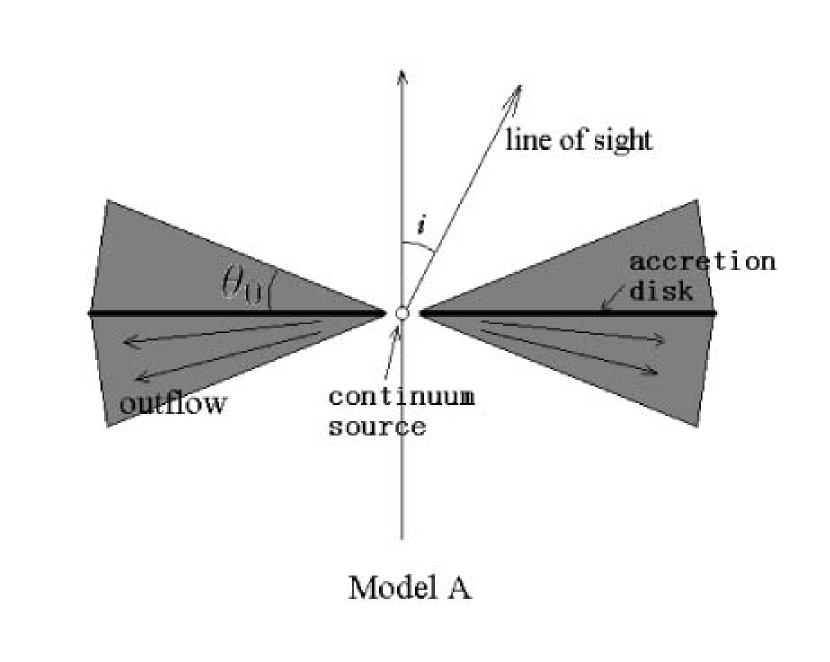
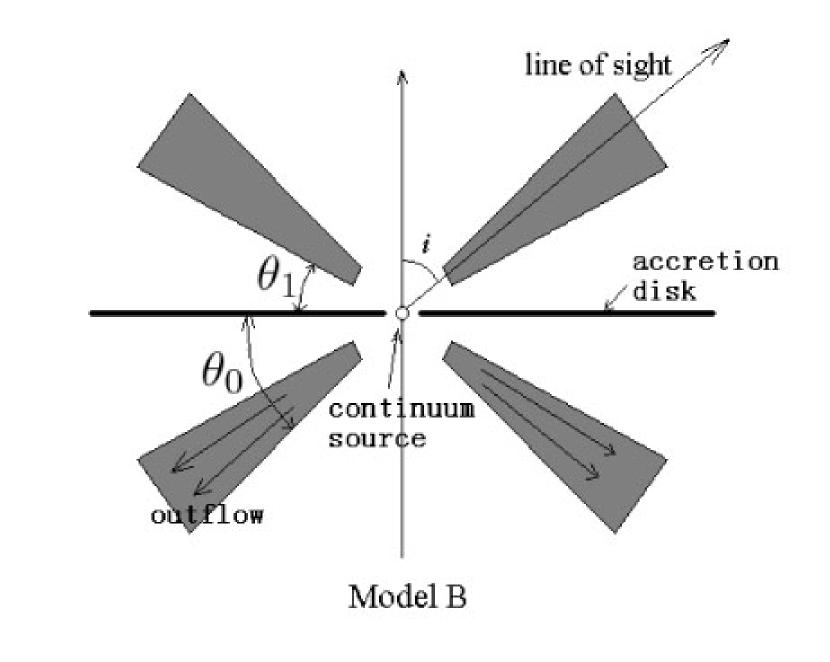
Figure 1: The cross section of the geometry of the outflow used in this paper. The thick line in the midplane is the accretion disk. The center circle denotes isotropic continuum source. The grey region represents the BALR which is outflowing. In model A the outflow is equatorial with a half open angle of $\theta_{0}$ and in model B the outflow covers the intermediate inclination angle. $\theta_{0}$, $\theta_{1}$ and viewing angle $i$ are defined in this figure.

We assume two different geometries for the outflow: model A) the outflow is equatorial, with a half open angle of $\theta_{0}$ (see upper panel of Fig. 1); model B) the axisymmetric outflow launches at intermediate inclination, covering the inclination angle between 90^o$-\theta_{0}$ to 90^o$-\theta_{1}$ (see lower panel of Fig. 1). Model A can be considered as a special case of model B with $\theta_{1}$ = 0. We consider two models of the incident continuum. In the first model, we assume that the incident continuum is emitted by a point source, and slightly polarized with $p=1$%, presumably arising from a small electron scattering region (hereafter SESR), e.g., the shielding gas, around the continuum source (see Paper I). Unless otherwise specified, the polarization PA is assumed to be parallel to the symmetry axis of the outflow (PA${}_{c}=$0^o, PA_c is the position angle of the polarization in the continuum), as introduced by scattering of an oblate distribution of electrons. In the second model, we assume that the electron scattering region locates just interior to the BALR, and we treat electron and resonant scattering simultaneously.

By ignoring the velocity in the polar angle direction, we determine the radial distribution of the density in BALR using the mass conservation law $nv_{r}r^{2}=const$, where $v_{r}$ is the radial velocity and $n$ is the particle density. We assume that the ionization does not change with the radius (see also LB97 and M95), thus the density of specific ions also follows $n_{i}v_{r}r^{2}=const$. This is expected for the dominant ions in the model of M95, in which the final ionization level is set by the cutoff of the incident continuum, instead of the ionization parameter.

We adopt M95’s description of the radial velocity distribution: $v_{r}=v_{\infty}(1-r_{f}/r)^{\beta}$, where $r_{f}$ is the launching radius and $v_{\infty}\approx\alpha\sqrt{GM_{BH}/r_{f}}/(1-\alpha)$(see M95 for details) is the terminal radial velocity. The inner radius of the BALR is set to $r_{0}$ ($r_{0}>r_{f}$). Note $\beta=0.5$ corresponds to a constant ratio of the radiative force to the gravitational one. The total optical depth of the resonant scattering at the frequency $\nu$ can be written as (e.g., Lee 1994)

$$\tau^{\prime}(x)=\frac{\pi e^{2}}{m_{e}c}f_{i}\frac{c}{\nu_{0}v_{th}}\phi(x)N_{i}$$ (1)

where $f_{i}$ is the oscillator strength, $\nu_{0}$ the frequency at the line center, $v_{th}$ the thermal velocity, $N_{i}$ the ion column density, $\phi(x)=1/\sqrt{2\pi}\exp(-x^{2}/2)$ is the absorption profile, and $x=\frac{(\nu-\nu_{0})}{\nu_{0}}\frac{c}{\upsilon_{th}}$. Notice that the average optical depth over the flow velocity,

$$\tau_{0}=\int\frac{\tau^{\prime}(x)v_{th}}{v_{\infty}-v_{0}}dx=\frac{\sqrt{2\pi}v_{th}\tau^{\prime}(0)}{\Delta v},$$ (2)

rather than the total optical depth, measures the saturation of the absorption line, whereas $v_{0}=v_{r}(r_{0})$ and $\Delta v=v_{\infty}-v_{0}$ are the initial velocity and the width of the absorption trough, respectively.

With these assumptions, the optical depth in the radial direction can be written as

$$\tau(v_{r})=\frac{\pi e^{2}}{m_{e}c}f_{i}\frac{c}{\nu_{0}}n_{i}(\frac{dv_{r}}{dr})^{-1}=\frac{\Delta v}{v_{r}}\frac{\gamma\tau_{0}}{(v_{r}/v_{0})^{\gamma}-(v_{r}/v_{\infty})^{\gamma}}$$ (3)

where $\gamma=1-1/\beta$. Note $\beta=0.5$ produces a constant optical depth over absorption line profile, or a boxy absorption line trough. The optical depth decreases for $\beta>0.5$ as velocity increases, and increases for $\beta<0.5$.

Since the flow is believed to be launched from the accretion disk, it must also carry angular momentum. Assuming no external torque and no shearing, we can determine the transverse velocity $v_{\varphi}$ according to the angular momentum conservation $rv_{\varphi}\sin{\theta}=r_{f}v_{\varphi,0}$, where $v_{\varphi,0}$ is the tangential velocity at the launching radius $r_{f}$. For a geometrically thin disk around a super-massive black hole, $v_{\varphi,0}$$=(GM_{BH}/r_{f})^{1/2}$ is the Keplerian velocity at $r_{f}$. Note that the $r_{f}$ and $v_{\varphi,0}$ should be taken as the radius, and the tangential velocity where the magnetic torque is no longer important in a magnetically launched wind (e.g., Konigl & Kartje 1994; de Kool & Begelman 1995). We introduce the rotation parameter $q=v_{\varphi,0}/v_{\infty}$ to describe the rotation of the outflow. In the following simulations, we will consider four different rotation parameters: 0.0, 0.25, 0.5 and 1.0. Hereafter, we use A$i$-$\theta_{0}$/B$i$-$\theta_{0}$-$\theta_{1}$ to distinguish different models, where $i$ stands for $4q$. For example, model A1-12^o represents model A with a rotation parameter $q$ =0.25 and $\theta_{0}=$12^o, and model B2-45^o-30^o for model B with $q=0.5$, $\theta_{0}=$45^o and $\theta_{1}=$30^o.

Once the outflow model is specified, it is straightforward to calculate the polarization. Same as Paper I, we denote the density of the polarized incident photons in direction $(\theta_{i},\varphi_{i})$ as

$$\left(\begin{array}[]{cc}\rho_{11}^{i}&\rho_{12}^{i}\\ \rho_{21}^{i}&\rho_{22}^{i}\end{array}\right)$$

where $\rho_{ij}$ is the $i$,$j$ component of the photon-density matrix. The outward density in the direction $(\theta_{o},\varphi_{o})$ is

$$\left(\begin{array}[]{cc}\rho_{11}^{o}&\rho_{12}^{o}\\ \rho_{21}^{o}&\rho_{22}^{o}\end{array}\right).$$

For the transition of singlet, such as the Be-like CIII$\lambda 977$, of which the ground state has $J=0$, we may write explicitly the outward photon density after one resonant scattering as $Eq.$ 1-4 of paper I (see also Chandrasekar 1950). Note most strong BALs are Li-like transitions, e.g., CIV $\lambda\lambda 1548,\;1550$Å  and NV$\lambda\lambda 1239,\;1243$Å. In these cases the ground level has $J=1/2$ and the two excited levels have either $J=1/2$ (the lower one) or $J=3/2$ (the upper one). For these transitions the density of the scattered photon relates to that of the incident photon by

$$\rho_{\beta\beta^{\prime}}\propto\sum_{\alpha\alpha^{\prime}}\sum_{ee^{\prime}}\sum_{gg^{\prime}}\textbf{\emph{M}}_{g^{\prime}e}(\textbf{\emph{e}}^{out}_{\beta})\textbf{\emph{M}}_{eg}(\textbf{\emph{e}}^{in}_{\alpha})\rho_{\alpha\alpha^{\prime}}\textbf{\emph{M}}_{ge^{\prime}}(\textbf{\emph{e}}^{in}_{\alpha^{\prime}})\textbf{\emph{M}}_{e^{\prime}g^{\prime}}(\textbf{\emph{e}}^{out}_{\beta^{\prime}})$$ (4)

where $\rho_{\beta\beta^{\prime}}$ and $\rho_{\alpha\alpha^{\prime}}$ are the density matrices of the scattered and the incident photons, respectively; $e$ and $g$ denote the sublevels of the exited and the ground states; and M is defined in $Eq.$ 2.6 of Lee et.al (1994). Following the procedures presented in Paper I, we calculate the Stokes parameters of the emergent photons for the given incident radiation and the spatial distribution of ions with Monte-Carlo simulations. By definition, only photons whose energy in the rest frame of the ion equals to the difference of the two energy levels can be resonantly scattered. Doppler shift due to the bulk motion and thermal motion has to be considered in the following calculation.

We calculate the four Stokes parameters $I$, $Q$, $U$, $V$ with Eq. 5 of paper I. Other quantities, such as the polarization degree, polarized flux and PA rotation, which can be observed directly, are calculated from the Stokes parameters according to the following formula:

$$p=\frac{\sqrt{Q^{2}+U^{2}}}{I},\;\;f_{p}=pI,\;\;\tan(2\mathrm{PA})=U/Q$$ (5)

where $p$, $f_{p}$ and PA are the linear polarization degree, polarized flux and polarization position angle, respectively. We do not consider the circular polarization because no measurement of circular polarization is available.

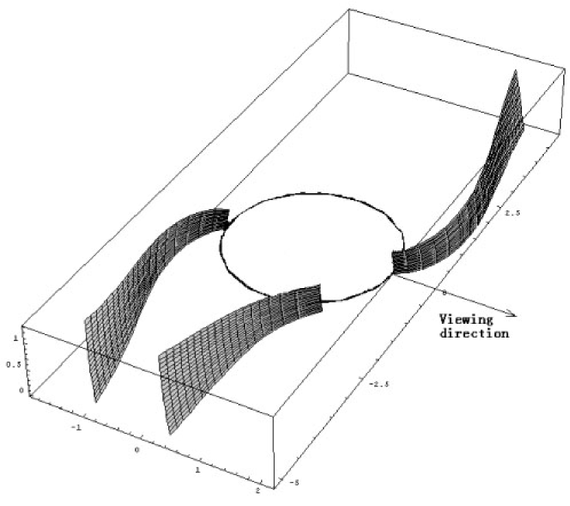
Figure 2: IVS for A-12^o model. The photons scattered in the three curved surfaces and escaped along the arrow have the same observed frequency. Because of the asymmetry of the IVS the PA is rotated.

For the resonant scattering, the optical depth $\tau^{\prime}$ is calculated using the Sobolev-Monte Carlo approach (LB97). The escaped photons are binned in frequency and the polar angle. The emergent photons with the same frequency in the given direction come from a curved surface with the same projected flow velocity along the line of sight (iso-velocity surface, IVS for short), rather than from the whole volume as in the case of electron scattering. If the flow has a transverse velocity, such as disk winds, the IVS is twisted (Fig. 2). This leads to the PA rotation as we will show below.

Recent works suggested that most common BAL region might be partially covered, and severely saturated with a typical optical depth $\tau_{0}>20-80$ for OVI, CIV, NV.(Hamann 1998; Arav et al. 1999; Wang et al. 2000). Meanwhile the material might be optically thin for rare elements. In this paper we will consider a wide range optical depths to include both cases. Since the polarization of the scattered light for singlet and doublet transitions is different (e.g., Blandford et al. 2002), we will treat them separately. We assume $\beta=0.5$ and $\Delta v/v_{\infty}\approx 0.8$ unless otherwise specified.

3 Singlet Transitions

3.1 Test of the Monte-Carlo Code

In the optically thin limit ($\tau<<1$), the polarization of resonantly scattered photons can be obtained analytically. By integrating the scattered photon density over the IVS described in §2, we obtain Stokes parameters at a specific velocity. With the relation between the scattered and incident photon density (Eq 1$\sim$4 of paper I), we obtain the polarization of the scattered photons at the line center for model A0 (i.e., $q$ = 0) as follows

$$p=\left\{\begin{array}[]{ll}0&(i<\theta_{0})\\ \frac{\sin(2\theta_{x})}{2\theta_{x}}&(i>\theta_{0}),\end{array}\right.$$

$$\theta_{x}=\arcsin(\frac{\sin\theta_{0}}{\sin i}),$$ (6)

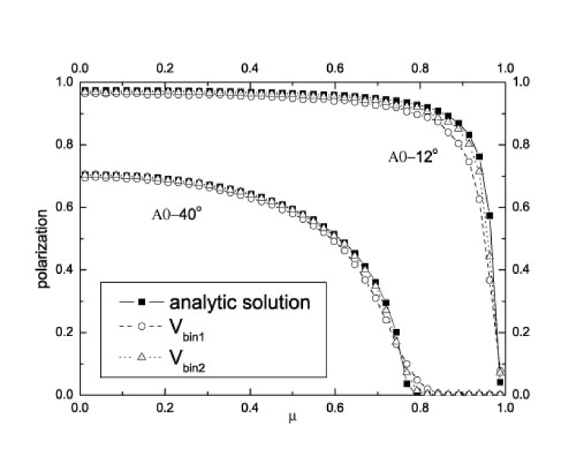
Figure 3: The polarization of the single scattered light for singlet transition at line center obtained in the simulation (open triangles and open circles) and the analytic solution (black squares) for a pure radial outflow (model A0-12^o and A0-40^o and a small electron-scattering region(SESR) see text for detail). The triangles and circles are for binsizes of $v_{bin1}=v_{\infty}/20$ and $v_{bin2}=v_{\infty}/10$, respectively. The discrepancy between the analytic solution and the simulation result especially seen from the polar direction is due to binning effect.

where $\theta_{0}$ and $i$ are defined in Fig. 1. Fig. 3 shows the results for $\theta_{0}$=12^o (equivalent to a covering factor 20$\%$, as inferred from the occurrence of BAL QSOs) and $\theta_{0}=40^{\rm o}$.

This analytic model is used to test our Monte-Carlo code. We run our Monte-Carlo code for this model, and the result is compared with the above analytic result (Fig. 3). The simulated polarization degree at the line center is consistent with the analytic one at large inclination angle, but substantially smaller at low inclinations if we adopt a velocity bin size $v_{\infty}/10$. The difference becomes very small for the bin size $v_{\infty}/20$. We consider the difference as a frequency-binning effect, in which the photons in a velocity bin come from a slice with a finite thickness instead of from an infinite thin surface, and the average over the IVS slices will bias toward small polarization. This effect is most significant when the gradient of polarization with respect to the viewing angle is largest. Therefore, we adopt a velocity bin size of $v_{\infty}/20$ in all the simulations below.

3.2 Small Electron-Scattering Region (SESR)

We first consider a polarized incident continuum with $p=1$%, presumably arising from an electron scattering region much smaller than the BALR around the continuum source. The incident continuum is considered as a point source and only resonant scattered is taken into account in the simulation. The density and velocity distribution of the BALR is described in §2.

3.2.1 Model A

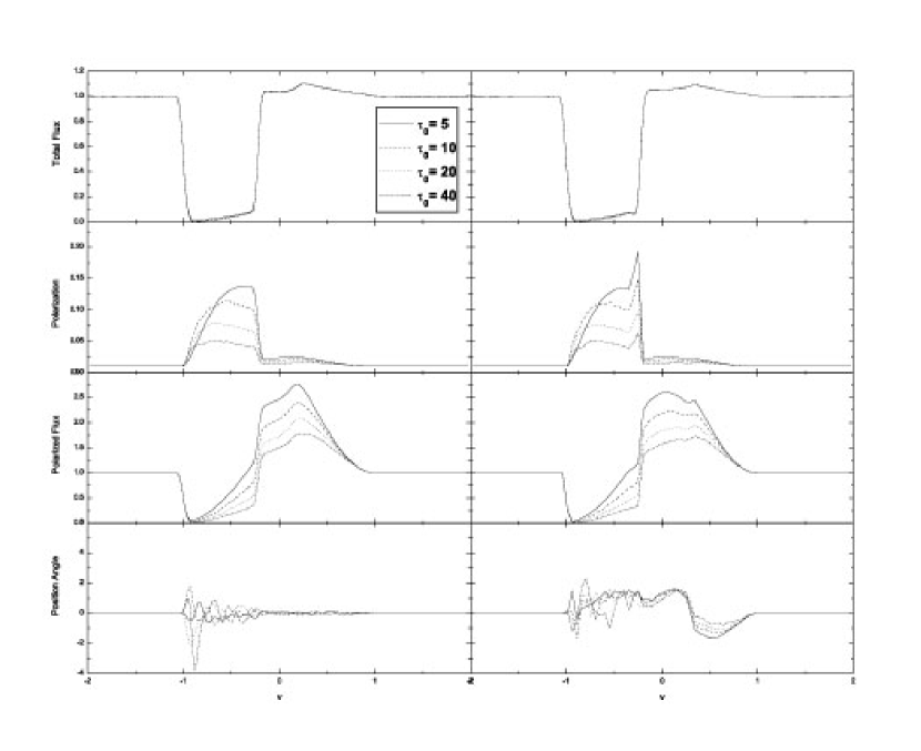
Figure 4: The average total flux, polarization degree, polarized flux and the PA for singlet in the velocity space for model A-12^o and a SESR, $\tau_{0}$=5,10,20,40. $q$ equals to 0 in the left panel and 0.25 in the right panel. Here all quantities are averaged over inclination angles for BAL QSOs.

We summarize the results for a radial outflow (model A0-12^o) in the left panel of Fig. 4. Obviously, the absorption line trough has much higher polarization than the continuum. The polarization degree in the line trough increases with increasing optical depth for small optical depths $\tau_{0}$ (see $Eq.$2), reaches a maximum of 14% at $\tau_{0}=5$, and declines at larger $\tau_{0}$. The rising of polarization at small $\tau_{0}$ is due to suppression of unpolarized transmitted light and falling at large $\tau_{0}$ is due to increasing importance of multiple scattering, which produces low polarization light. BAL trough is visible in the polarized flux, but is shallower and skewed to the blue side than in the total light. This is caused by the combination of several factors. First of all, the polarized incident continuum was resonantly scattered in the BALR, leaving an absorption trough in the polarized flux. Second, the resonantly scattered line photons from other directions fill the trough. Note that the polarization degree of the scattered light is higher at lower velocities for small and moderate optical depths ($\tau_{0}=5$) because the IVS locates closer to the direction perpendicular to the line of sight. In addition, there is much less scattered photons at large velocities because the ions in the IVS slice becomes smaller as the velocity increases. To the red side of the absorption trough, there are excess emission in the polarized flux due to resonantly scattered light, which has the same PA as the continuum polarization. The peak of the scattered light is in the red side of emission line around $v_{0}$. We note that no rotation of PA relative to the continuum is produced. The large PA fluctuation at large velocities for large $\tau_{0}$’s in Fig. 4 is due to photon statistics because only a small number of photons are collected at large velocity for A0 model.

Next we consider the effect of the rotation of the flow. There is no direct observational constraint on the value of $q$. However, if the wind is launched thermally or hydrodynamically from a Keplerian disk, $v_{\varphi,0}$ is the Keplerian velocity at the launching radius. With the model describing in §2, the starting site of BALR is close to $r_{f}$. Since very often the broad emission lines are also absorbed by BAL, $r_{f}$ should be no less than the size of BLR. This sets an upper limit on $v_{\varphi,0}$ to within a factor of two of the broad line width if the latter is virialized. This suggests $q\sim 0.25--0.5$. On the other hand, if the wind is launched hydromagnetically, then $v_{\varphi,0}$ has to be redefined as the rotational velocity at the site where the magnetic torque is no longer important. The velocity should be larger than the local Keplerian velocity. In the following analysis, we will consider $q$=0.25, 0.5 and 1.0 (corresponding to model A1-12^o, A2-12^o and A4-12^o).

The simulated results are summarized in Fig. 4 and 5. Obviously, the rotational velocity causes a rotation in PA in the scattered light. The PA rotation is nearly constant over the absorption trough, but swings from positive to negative rotation to the red-side of the emission line. PA rotation in the trough does not depend strongly on the optical depth. It increases with $q$ because it is sensitive to the distortion of the IVS, which is determined by the angular velocity, thus $q$. The rotation also produce a sharp peak in the polarization between $v_{0}$ and $qv_{\infty}$. The peak is caused by an additional Sobelov surface at projected velocities $<qv_{\infty}$ (Fig 2.) and an increase in the velocity gradient between projected velocity $v_{0}$ and $qv_{\infty}$. The contribution from additional Sobelov surface also bring the peak in the polarized flux very close to $v_{0}$.

3.2.2 Model B

The structure of a quasar might be similar to that of Seyfert galaxies, in which the line of sight to the equatorial direction is believed to be blocked by a thick dusty torus (e.g., Antonucci 1993; Dong et al.2005; Martínez-Sansigre et al. 2005). In the case, BAL QSOs are viewed only at intermediate inclinations, and the BALR might be confined to intermediate polar angles. Similar situation arises when the absorbing material is launched vertically first, and then accelerated radially by the radiation pressure (see Elvis 2000). In these scenarios, the flow can be approximately described as model B-$\theta_{0}$-$\theta_{1}$ (see Fig. 1).

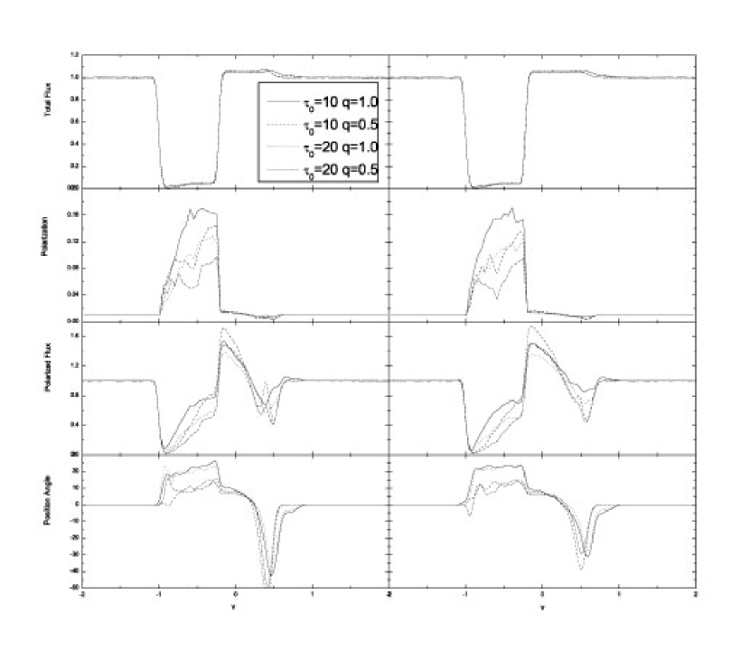
Figure 6: The total flux, polarization degree, polarized flux and the PA for singlet in the velocity space for model B-33^o-20^o and a SESR, viewing from $i=57^{\rm o}$(left panel) and $i=70^{\rm o}$(right panel ). $\tau_{0}$ and $q$ are marked in the figure.

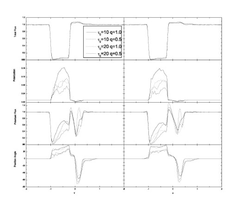
Figure 7: Similar to Fig. 6 but for model B-45^o-30^o viewing from $i=45^{\rm o}$(left panel) and $i=60^{\rm o}$ (right panel).

In Figs. 6 and 7, we show results for model B-33^o-20^o and B-45^o-30^o with different $\tau_{0}$ and $q$. In general, polarization degree and polarized flux in the absorption line trough looks quite similar to type-A models: a more highly polarized and blue-skewed trough, a jump in polarization degree around $qv_{\infty}$, and PA rotation across the line profile. There are also several important differences between the two models. First, type-B models produce much larger PA rotation in the trough, about 27^o for B4-33^o-20^o and 40^o for B4-45^o-30^o. It is easy to understand because the distortion of the IVS becomes larger due to the angular momentum conservation. Second, an additional absorption trough appears to the red side of the emission line in the polarized flux (see details in Appendix A and discussion below). Subsequently, the excess of polarized flux around $v_{0}$ is narrow. The PA rotation is particular large in the this trough with a negative value. The resonant scattering light is also more blueshifted than that in type-A models, as such more scattered photons fill into the trough.

Combining the results of model A and B, we find the polarization properties (PA, polarized degree, polarized flux and PA) are sensitive to the rotation parameter $q$ and the geometry of the model. As in model A, $q$ significantly affects the PA rotation and the polarization degree in the trough, while the optical depth alters only the polarization degree and the polarized flux but not for the PA rotation in the trough.

3.3 Large Electron-Scattering Region (LESR)

Now we consider the case that the shielding gas, as the inner part of the outflow, locates just interior to the inner region of BALR. In this case, we assume an unpolarized incident continuum, and simulate the electron scattering in the shielding gas and the resonant scattering in the BALR outflow simultaneously. Same as in Paper I, we adopt a constant density model for the shielding gas with an electron column density of $N_{e}=4\times 10^{23}$ cm^-2 and the same sky coverage as the BALR for model A-12^o, $N_{e}=3\times 10^{23}$ cm^-2 and covering factor=$\sin\theta_{0}$ for model B. With these parameters, the expected continuum polarization is around 1%, thus directly comparable to the SESR models.

3.3.1 Model A

Fig. 8 presents the polarization degree, the polarized flux, PA rotation and the total flux for model A-12^o. As expected, the continuum polarization degree is around 1% and its position angle is aligned with the symmetric axis. These results retain some of feature of the corresponding SESR models, such as excess polarization in the velocity range $-v_{\phi,0}$-$-v_{0}$, PA rotations for none-$q$ models. However, we find that the polarization degree in the trough is higher and decreases more slowly with increasing $\tau_{0}$ than in the model A-12^o with SESR. We also notice that the absorption trough appears only to the blue side of $v\simeq-v_{\varphi,0}$ in the polarized flux, and the PA rotation has no apparent jump around $-v_{0}$, which appears in the SESR models. These characteristics are remarkably different from models with SESR discussed in §3.1.1.

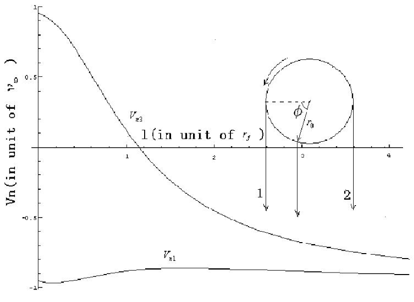
Figure 9: The projected velocity of the flow encountered by the photons from two sites towards the observer. The circle denotes the outer edge of the electron scattering region or the inner edge of the outflow. $\upsilon_{n1}$ is the projected velocity on the path 1 and $\upsilon_{n2}$ on the path 2. Obviously, photons only in a narrow frequency range are scattered by ions along the path 1, and photons with a wide range of frequence can be scattered along the path 2.

It should be pointed out that the differences arise because the ’leaked’ electron-scattered photons fill the trough. This is illustrated in Fig. 9, which shows the LOS(line of sight) velocities of the outflow along the track of the photons scattered by electrons at two different sites (marked by 1 and 2) at the equatorial plane. In the figure, the velocity towards us is taken as negative and away from us as positive. When the rotation of the flow is considered, photons with $\delta\lambda/\lambda_{0}$ in [-$v_{\infty}/c$, $v_{\varphi,0}/c$] may be scattered by ions along track 2, while only those with $\delta\lambda/\lambda_{0}$ in [-$v_{\infty}/c$,-$v_{\varphi,0}/c$ ] may be scattered along track 1, where $\lambda_{0}$ is the absorption wavelength of the ion in the rest frame. In other words, photons with $\delta\lambda/\lambda_{0}$ in [-$v_{\varphi,0}/c$, $v_{\infty}/c$] will reach the observer freely along track 1. For a general track crossing the circle of radius $r_{f}$ at $\phi$ (defined in Fig. 9, in the equatorial plane for simplicity), the scattered continuum in the wavelength range of $\delta\lambda/\lambda_{0}$ in [-$v_{\infty}/c$, -$(v_{0}\sin\phi$+$v_{\varphi,0}\cos\phi)/c$] will be absorbed. It is interesting to observe that the starting wavelength of resonant absorption to the electron scattered photons varies from $-v_{\varphi,0}$ (at $\varphi=0$) to $-v_{0}$ (at $\varphi=\pi/2$) then to $v_{\varphi,0}$ ($\varphi=\pi$) as we look at the electron scattering sphere from left to right in Fig. 9. Since the variation is smooth, there is no jump in the polarized light at $v_{0}$. In comparison with SESR models, the polarized flux in the velocity range [-$v_{\varphi,0}$, -$v_{0}$] is enhanced due to the contribution of leaked scattered continuum, whereas it is reduced in the velocity range [-$v_{0}$, $v_{\varphi,0}$] due to absorption of scattered light in the left half BALR region. If rotation velocity is comparable to $v_{\infty}$, the electron-scattered light will fill almost the entire trough except around $-v_{\infty}$, leaving a narrow absorption trough there in the polarized light (the left panel of Fig. 8).

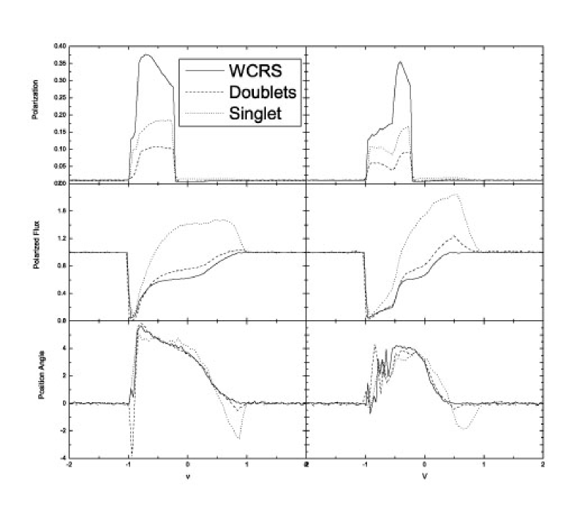
Figure 10: The polarization degree, polarized flux and the PA in velocity space for WCRS, singlet and doublets model. All are with a LESR. The left panel is for model A4-12^o and right one is for model A2-12^o. $\tau_{0}=20$ for both doublets and singlet.

To further support this analysis, we plot the polarized flux, its position angle and polarization degree of electron scattering light (labelled WCRS, without the contribution of resonant scattering) in Fig. 10. It includes the transmitted light from electron scattering region. The polarized flux rises almost linearly in the velocity range [$-v_{\infty}$, $\sim-v_{\varphi,0}$], presumedly due to variation in the optical depth, then increases very rapidly around $-v_{\varphi,0}$, reachs a plateau, and it increases to the continuum level at about $v_{\infty}$. The position angle of the scattered continuum rotates across the line profile in a manner similar to the resonantly scattered light because at a given frequency the leaked region is no longer rotationally symmetric.

In Fig. 10, we also show the final polarization degree, polarized flux, and position angle to illustrate the relative contribution of the leaked light. It is obvious that the leaked light is more polarized than resonantly scattered light because of large line optical depth considered in the model (panel A). The relative importance of the leaked continuum depends on the line optical depth, and become more important at large optical depth because the polarization of resonantly scattered light decreases with increasing optical depth while that of leaked continuum does not. As a result the polarization degree is less sensitive to optical depth in a LESR model than the corresponding SESR model. For example, the highest polarization in the trough drops from 21% to 8% (a factor of $\sim 2.6$) when $\tau_{0}$ increases from 5 to 40 for A4-12^o model with SESR. It changes only 50% for the same model with LESR.

At small $q$, such leakage is insignificant. An apparent jump appears around $v=-v_{\varphi,0}$ in the polarization: the polarization is larger at $v>-v_{\varphi,0}$ and smaller at $v<-v_{\varphi,0}$ (Fig. 8). Similar jumps also appear in the panels of the polarized flux and the PA. These jumps are caused by the fact that the leakage contributes mostly to the polarized flux at $v>-v_{\varphi,0}$, whereas resonantly scattered light works at at both large and small velocities.

3.3.2 Model B

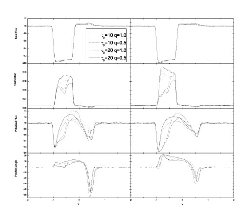
Figure 11: The total flux, polarization degree, polarized flux and the PA for singlet in the velocity space for model B-33^o-20^o and a LESR . The left panel is viewing from $i=57^{\rm o}$ and the right one is viewing from $i=70^{\rm o}$. $q$ and $\tau_{0}$ are marked in the figure.

We show the results in Fig. 11 (for model B-33^o-20^o) and 12 (for model B-45^o-30^o). The effect of LESR on type-B models is quite similar to that on type-A models, and can be attributed mainly to the ’leakage’ of the scattered continuum. For instance, the jump in the polarized flux, PA rotation in the SESR models at $v=-v_{0}$ is now replaced by a smooth profile. Polarized flux rises steeply at $v\simeq-v_{\varphi,0}$ due to the selective leakage.

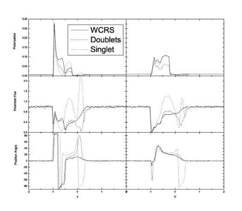
Figure 14: Similar to Fig. 13 but for model B2-45^o-30^o.

However, model B-45^o-30^o shows several distinctive characteristics that do not appear in previous models. First, PA swings from parallel to nearly perpendicular at $v\simeq-v_{\infty}$, and then back to parallel at $v\simeq-0.8v_{\infty}$ at viewing angle $i=45$^o . At large inclinations, the PA rotation appears smaller. Another PA swing of 90^o occurs at $v>0$. To understand the origin of these characteristics we plot the polarization degree, polarized flux and PA of models for doublet, singlet and WCRS in Figs. 13 and 14. From these figures, we easily find that the blue PA swing is caused by the electron scattering and the red PA swing is due to the resonant scattering.

In the previous section we introduce two polarizing processes in the line trough, resonant scattering and selective leakage. Here, an additional process, back-scattering of electron in the shielding gas, is also important for model B, especially at large $\theta_{0}$. In model A with small $\theta_{0}$, most of back-scattering photons intercept the BALR, whereas in model B only photons with velocity $\sim-v_{\infty}$ intercept the BALR, and others do not, thus fill the trough directly. The polarization, polarized flux and PA rotation are determined by the competition among the three processes. In order to investigate the back-scattering we integrate electron-scattering photon density in the region with 90${}^{\rm o}<\varphi_{i}-\varphi_{o}<270^{\rm o}$ according to $Eq.$ 1-5 of Paper I and obtain the Stokes parameters Q of the back-scattering photons:

$$Q_{bs}\propto\frac{\pi}{2}\sin\theta_{0}\sin^{2}i(1-\sin^{2}\theta_{0})-\frac{2}{3}\sin 2i(1-\cos^{3}\theta_{0})$$ (7)

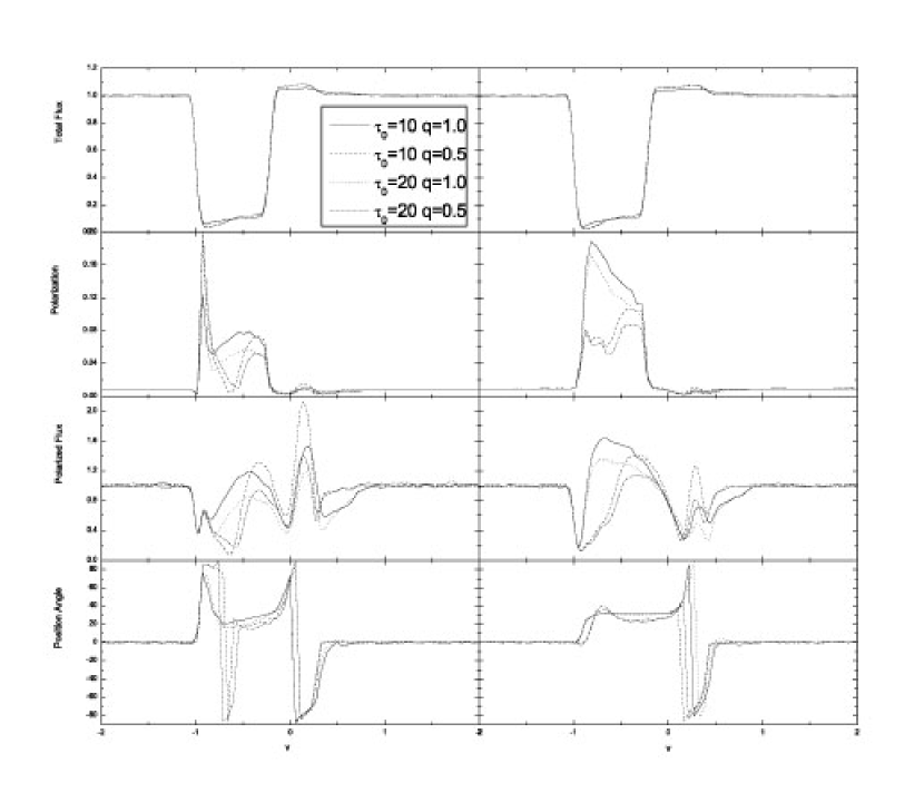
Figure 12: Similar to Fig. 11 but for model B-45^o-30^o viewing from $i=45^{\rm o}$(left panel) and $i=60^{\rm o}$(right panel).

This equation tells that the back-scattered light has always $Q_{bs}>0$ (i.e. polarization parallel to the symmetric axis) when models A-12^o and B-33^o-20^o are viewed at the BALR directions ($90$^o$-\theta_{0}\leq i\leq 90$^o). However, the polarization can be either parallel, i.e., $Q_{bs}>0$ at $i=60$^o, or perpendicular to the symmetric axis, i.e., $Q_{bs}<0$ at $i=45$^o for model B-45^o-30^o. Furthermore the selective leakage is working only at $v>-v_{\varphi,0}$ (see §3.2.1) while most resonantly scattered photons will be at small velocities (see §3.1.1), therefore, back-scattering can dominate the polarized light in the blue part of trough. This explains why the blue PA swing appears only in the model B-45^o-30^o viewed at $i=45^{\rm o}$ for all cases considered. Our interpretation is verified by our simulation and presented in Fig 12.

The red PA swing (Figs. 11 and 12) is caused by the same reason as the sub-trough for model with SESR. We will discuss this in details in the next section.

4 Doublet Transitions

In this section we will simulate the resonant scattering for doublets, and compare the results with those for singlets. As an example, we consider the two transitions of CIV: $J=1/2\rightarrow 1/2$ ($T_{1/2}$, $\lambda=$1550Å) and $J=1/2\rightarrow 3/2$ ($T_{3/2}$, $\lambda$=1548Å). The cross section of the former transition is 1/2 of the latter. According Eq. 4, the scattered light of $T_{1/2}$ transition is unpolarized regardless the polarization of the incident light.

4.1 Small Electron Scattering Region

4.1.1 Model A

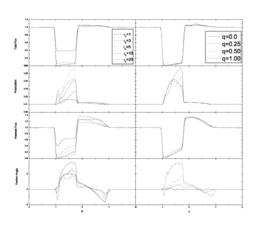
Figure 15: Total flux, polarization degree, polarized flux and the PA of polarization for scattering of doublet transition. The model adopt is A-12^o and a SESR. In the left panel, $q=1.0$ is constant and different $\tau_{0}$ is marked. And in the right panel, $\tau_{0}=5$ and different $q$ is marked. Here all the four quantities are the average value over viewing angle for the BAL QSOs.

We first make simulations for model A4-12^o with total optical depths of the doublets $\tau_{0}$=1, 3, 5, 10, 20. The output PA, polarization degree and polarized flux are showed in Fig. 15. In many aspects, the scattering of doublets produce similar characteristics as the scattering of singlets but at reduced polarization degree: PA rotation and asymmetric profile of PA rotation at moderate and large optical depths, larger polarization in the trough than in the continuum, a shallower trough in the polarized flux and the excess of the polarized flux across the emission line position. However, there are apparently differences too. First, the polarization degree is greatly reduced, with a maximum of only $6.0\%$ at $\tau_{0}=5$. Second, the PA rotation decreases with increasing optical depth for $\tau_{0}>5$ though the maximum ($\sim 5$^o for model A4-12^o) is similar to that for singlet.

The differences can be understood as follows. For an accelerating outflow, the continuum photons encounter the scattering surface of $T_{3/2}$ transition first then the $T_{1/2}$ transition surface, which will erase the polarization produced by $T_{3/2}$ surface (Blandford et al. 2002), especially, at large optical depth. As a result, the final polarization degree is greatly reduced, and is essentially determined by the optical depth of $T_{1/2}$ surface when $\tau_{0}$ is moderate or large. As the optical depth increases, the erasion of polarization by $T_{1/2}$ scattering surface is more effective in the inner region, where large PA rotation of the scattered light from $T_{3/2}$ surface is produced. This leads to a decrease of PA rotation with the increase of optical depth.

High polarization in CIV and NV troughs observed in some BAL QSOs requires rather small $\tau(v)$ for the transition $T_{1/2}$, at least in a significant part of the flow if the polarization is attributed to the resonant scattering. For the models described in §2, if $\beta$ is substantially larger than 0.5, the optical depth $\tau$ in radial direction will drop rapidly outward (Eq. 3), and eventually becomes quite moderate at large radii, to the transition $T_{1/2}$ even the inner region is optically thick. The Monte-Carlo simulations have been carried out for $\beta=$0.75, 1.5, 2.0 and $\tau_{0}=3$. We find that the maximum polarization increases with increasing $\beta$, and reaches $\sim$ 9% for $\beta=2$. We also made simulations for different $\theta_{0}$, and find that the polarization degree decreases slightly and PA rotation increases with increasing $\theta_{0}$ in the optically thick cases. The reason is that the flux in the trough is already dominated by the scattered light, of which the polarization decreases slightly with increasing $\theta_{0}$. These results illustrate that the polarization depends much more strongly on the velocity structure than on $\theta_{0}$ for a moderate or large optical depth.

LB97 considered an equatorial outflow that is accelerated on hyperboloid surfaces, and obtained a higher maximal polarization in the trough, 50% for singlets and 15% for doublets (10% when rotation is included). The main cause for such difference is that they adopted a different prescription of the flow that moves in poloidal (and azimuthal) direction as such the velocity along the line of sight is non-monotonic. They also got a small polarization ($\simeq$ 10% for singlets) for velocity law $v_{r}\propto r$.

4.1.2 Model B

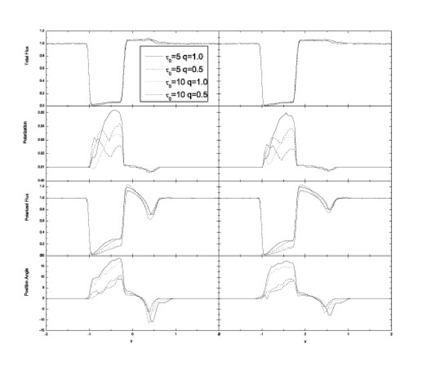
Figure 16: The total flux, polarization degree, polarized flux and PA for doublets . The model adopted is B-33^o-20^o and a SESR. The left panel is viewing from $i=57^{\rm o}$ and the right one is viewing from $i=70^{\rm o}$. $\tau_{0}$ and $q$ are marked in the figure.

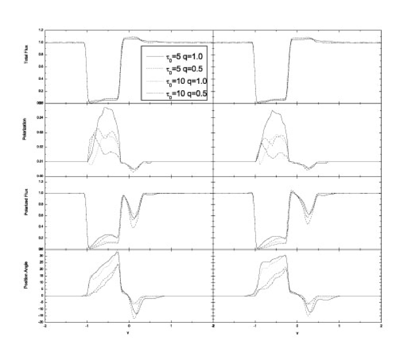
Figure 17: Similar to Fig. 16 but for model B-45^o-30^o, viewing from $i=45^{\rm o}$(left panel) and $i=60^{\rm o}$(right panel).

The numerical results for models B-33^o-20^o and B-45^o-30^o are summarized in Table 1 and shown in Fig. 16 and Fig. 17.

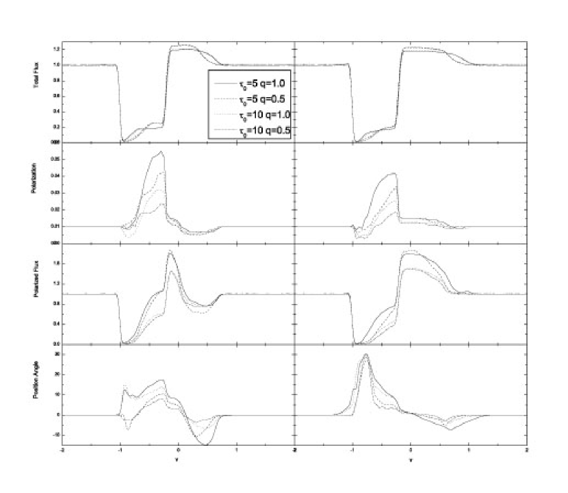
Figure 18: Similar to Fig. 16 but for model A-45^o, viewing from $i=45^{\rm o}$(left panel) and $i=90^{\rm o}$(right panel).

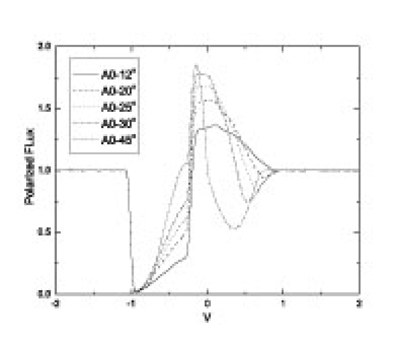
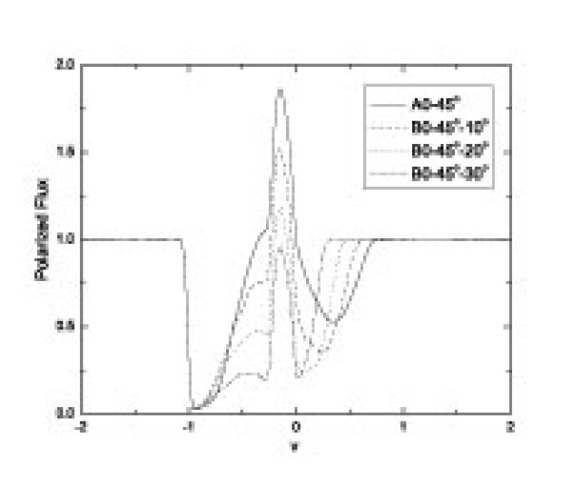
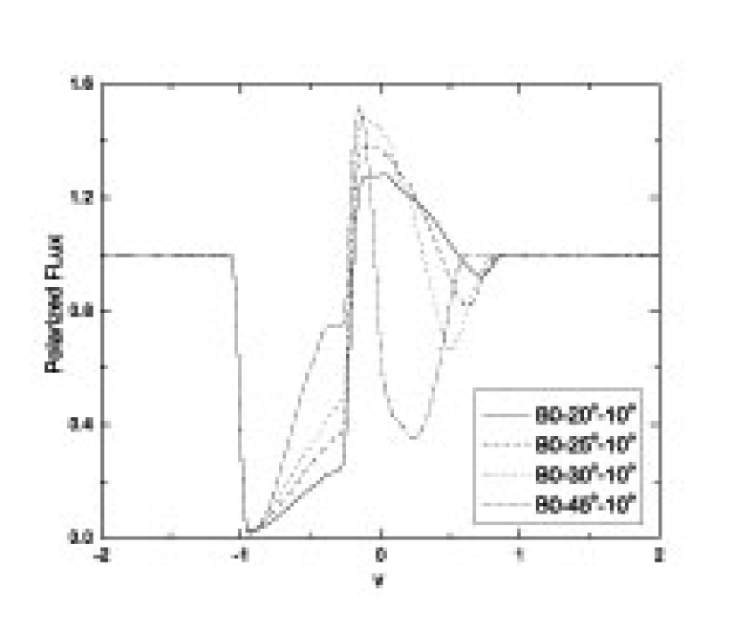
Figure 22: Polarized flux from scattering of doublets for different $\theta_{0}$ and $\theta_{1}$ viewed from $i=90$^o$-\theta_{0}$. $\tau_{0}=5$ is assumed in all models and with a SESR on the base of the outflow.

Similar to singlet models, an additional absorption trough appears to the red side of the trough in the polarized flux. This sub-trough is especially prominent for large $\theta_{0}$’s and at small inclinations. As $\theta_{0}$ decreases and viewing angle increases, it becomes shallower and moves to the red side, and an emission-line like feature appears around $v=0$. PA rotation is also much larger than those in model A-12^o and can reach as high as 30^o for $\theta_{0}=45$^o when $\tau_{0}=5$. From Fig. 18, it is clear the PA rotation across the profile is sensitive to the inclinations as well. PA rotation peaks at small velocities at small inclinations, but the peak shifts to the blue part of the trough at large inclinations. However, large PA rotation and the appearance of the red sub-trough in the polarized light is a characteristic of all models with large $\theta_{0}$, rather than of type B-models only (Figs. 18 and 22). But the shape of sub-trough is different for type-A and for type-B models: broad for type-A models and narrow for type-B models. A comparison of polarized line profile for different models is given in Fig. 22. We find that when $\theta_{0}$ increases the sub-trough becomes broader and deeper, and shifts to the blue-side. As $\theta_{1}$ decreases it gets broader and shallower and shifts to the red side, and an emission-line like feature appears due to the scattered photons from the low latitude. Only models with large $\theta_{1}$ can produce an apparent sub-trough, which is much narrower than the primary trough.

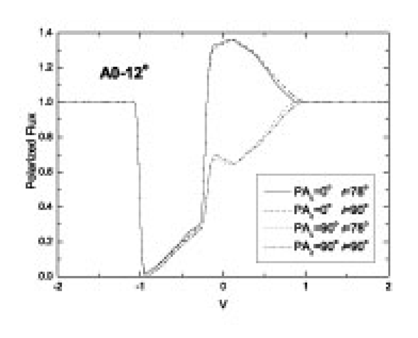
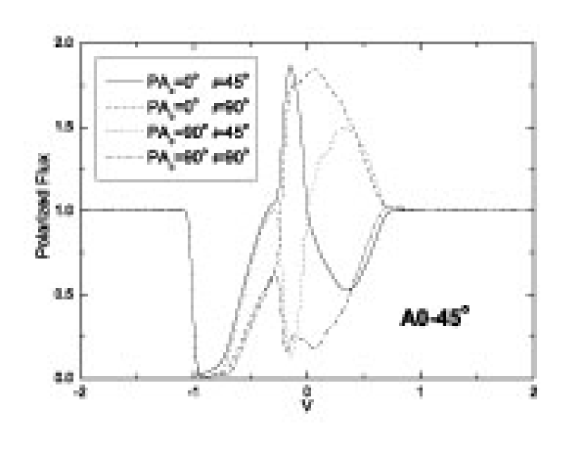
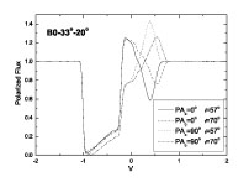
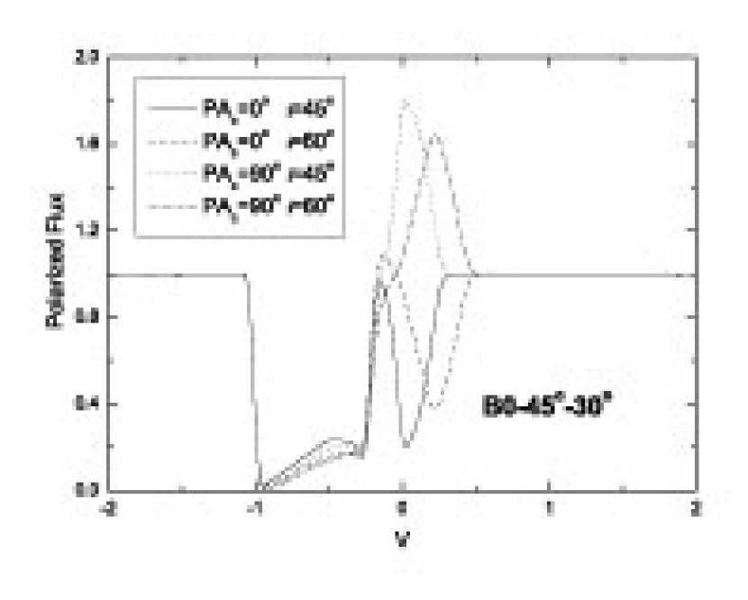
Figure 23: Polarized flux from scattering of doublet for two incident continuum polarization, PA${}_{c}=0$^o and PA${}_{c}=90$^o, and for model A0-12^o, A0-45^o, B0-33^o-20^o and B0-45^o-30^o. $\tau_{0}=5$ is assumed.

The red sub-trough in the polarized flux actually is not due to absorption, but result from the cancellation of the continuum polarization by the scattered polarized line flux as shown in Appendix A. In the Appendix, we demonstrate that the necessary condition for the appearance of the sub-trough is $\theta_{0}\gtrsim 25^{\rm o}$ regardless the rotation velocity of the flow. Hence the appearance of this feature sets a lower limit on $\theta_{0}$. We also compare the numerical results for models A0-12^o, A0-20^o, A0-25^o, A0-30^o & A0-45^o with models B0-20^o-10^o, B0-25^o-10^o, B0-30^o-10^o, B0-33^o-20^o & B0-45^o-30^o, and find a sub-trough in the polarized flux only in models with $\theta_{0}\geq 25^{\rm o}$ (Fig. 22). Numerical results in Fig. 22 and Fig. 23 (PA_c=0^o) also confirm that even if $q=0$ the sub-trough also appears. The sub-trough in the A0 and B0 models appears to be deeper than that of the A4 and B4. But the depth of the sub-trough depends on optical depth and is inversely proportional to the continuum polarization.

The numerical results are summarized in the Table 2 for $\tau_{0}=5$ and four different $q$’s, and some of them are plotted for comparison (Fig. 16 and 17). PA rotation increases with increasing $q$, as for singlets, and depends strongly on $\theta_{0}$. The maximum polarization in trough, about $4\%\sim 6\%$, decreases slightly with increasing $\theta_{0}$ and increases with increasing $q$, same as what we noticed in previous section.

Table 1: Maximum PA rotation(PA_m) and polarization($P_{m}$) for different models

$4\times q$	1	2	3	4
		PAm
A-12o	–	2o$\sim$3o	–	3o$\sim$5o
A-30o	2o$\sim$8o	5o$\sim$12o	6o$\sim$14o	9o$\sim$16o
A-45o	3o$\sim$24o	7o$\sim$28o	12o$\sim$32o	16o$\sim$31o
B-33o-20o	4o$\sim$6o	8o$\sim$11o	13o$\sim$16o	15o$\sim$19o
B-45o-30o	10o$\sim$14o	21o$\sim$26o	28o$\sim$34o	31o$\sim$35o
		$P_{m}$
A-12o	4.5%	4.9%	5.5%	6.0%
A-30o	4.3%	4.8%	5.4%	5.9%
A-45o	3.8%	4.2%	4.8%	5.5%
B-33o-20o	4.2%	4.2%	4.8%	5.2%
B-45o-30o	3.9%	3.3%	4.0%	4.8%

4.2 Large Electron-Scattering Region

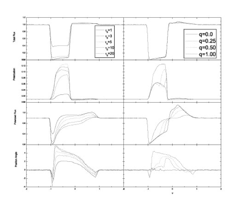
Figure 19: Similar to Fig. 15 but for LESR.

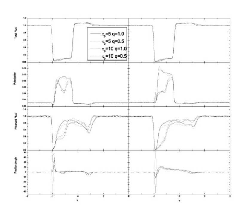
Figure 20: Similar to Fig. 16 but for LESR.

For doublets, we carry out simulations also for LESR models. The results are shown in Fig. 19 for type-A models, Fig. 20 and 21 for type-B models. Due to the erasion of $T_{1/2}$ transition, the electron scattered light dominates the polarized flux in the trough when $\tau_{0}$ is large. As a result, the polarized flux and PA rotation are more similar to WCRS models than singlet models, whereas the summed polarization of the resonantly and electron scattered photons is lower for doublets than for singlets.

As demonstrated in the Appendix A, when $\theta_{0}$ is large enough the Stokes parameter $Q_{l}$ for the resonantly scattered light at positive $v$ becomes negative, i.e., PA_l is about 90^o. For SESR models with polarization of the incident continuum $\sim$1%, $|Q_{l}|$ is generally smaller than $|Q_{c}|$ in the entire velocity range, as such the final polarization has the same direction as the continuum (PA${}_{c}\sim 0^{\rm o}$) and only a sub-trough appears to the red side of the line center. However, in LESR models, part of red-shifted scattered continuum is absorbed so that $|Q_{l}|$ in the bottom of the sub-trough may be larger than $|Q_{c}|$. This leads to PA${}_{l}=90^{\rm o}$ and a local excess of the polarized flux at these velocities (Fig. 11, 12 and 21). If $|Q_{l}|>2|Q_{c}|$ the peak is higher than the polarized flux of the continuum (see Eq. 1 in Appendix A). We find such cases only for singlet models (Fig. 12). This feature appears only in certain geometry models and for certain ranges of $\tau_{0}$ and continuum polarization degree.

To summarize, resonant scattering of doublets usually produces much lower polarization at large optical depth for accelerating flows. The polarization degree is sensitive to the velocity law. A slowly accelerating flow (large $\beta$) or non-monotonic velocity in radial directions will produce higher polarizations. Models with LESR can easily produce high polarization due to back-scattering and leakage of the electron scattered continuum. Large PA rotation can be reproduced only by a rotating outflow with a large $\theta_{0}$ for either SESR or LESR. Models with large subtending angle $\theta_{0}$ can produce a sub-trough to the red side of the primary trough in the polarized flux regardless the rotation velocity. A jump appears in PA rotation and polarized flux across the starting velocity of the outflow in SESR models, but it disappears in LESR models. The absorption to the polarized flux can extend to $v=v_{\varphi,0}$ at the red side of the line center for LESR models at large $\tau_{0}$.

5 Comparison with Observations

5.1 Polarization Degree

The observed polarization degree in the BAL line troughs vary from non-detection to up to 20% for strong doublets such as CIV and NV (O99). While the polarization degree at a few percent level can be reproduced by most models considered, polarization degree higher than 10% for doublets detected in a few objects puts severe constraints on the models. Below we will discuss three possible models that may reproduce such high polarization: a decelerating flow, a flow with a velocity law similar to that of LB97, and a large electron-scattering region.

Although it is generally believed that the outflow is accelerating, there is no compelling evidence against a possible decelerating region in the outer part of the flow (Voit, Weymann, & Korista 1993). Such non-monotonic velocity is observed in outflows of a handful Seyfert galaxies on sub-kpc scales (e.g, Ruiz et al. 2001). We notice that recent X-ray observations have revealed X-ray BALs which require massive outflow with higher velocities at radii smaller than UV BALR (Chartas et al. 2002; 2003). This also supports the existence of a decelerating region in the outflow. High polarization will be produced because the continuum photons are scattered by the surface of transition $T_{3/2}$ after they encountered $T_{1/2}$ so that the polarized light produced by scattering of the transition $T_{3/2}$ can reach us freely. With respect to scattering by singlet, there are two differences. First, the effective optical depth used to produce the polarized flux is contributed by the transition $T_{3/2}$ only, substantially lower than the total optical depth. Second, the photons reaching $T_{3/2}$ surface is a combination of transmitted light (through $T_{1/2}$ surface) and the scattered light, which appears much more isotropic to the scattering ions.

LB97 showed that large polarization can also be produced in a monotonic accelerating flow which follows a different prescription of velocity-law. As mentioned in previous section the velocity along the line of sight is also non-monotonic in their model. In previous section, we find models with a LESR can also produce high polarization degree because electron-scattered photons can fill the troughs and increases the polarization.

Ly$\alpha$ is actually a special doublet, in which fine structure splitting is very narrow, about 1.3 km/s, comparable to the thermal velocity. In that case, the polarization can be much higher because there is a good chance that polarized scattered photons (from $T_{3/2}$) escapes before encountering $T_{1/2}$ scattering. However, some of these escaped photons will be scattered again by NV at ISV surface with a velocity difference of -5,900 km s^-1 from the current Ly$\alpha$ scattering surface, so that their polarization will be erased again. At high altitude, the back-scattered light usually do not meet the NV scattering surface, and produce an excess in polarized flux in the red side of the Ly$\alpha$ emission line. The polarization in the overlap region of NV and L$\alpha$ is not as high as expected for the scattering of Ly$\alpha$ alone, but in general be higher than the pure NV scattering because a fraction of scattered Ly$\alpha$ photons comes directly. Since scattering by NV occurs after Ly$\alpha$ scattering, it is proper to consider the NV scattering with the incident light including scattered L$\alpha$ photons in the overlapped wavelengths. At flow velocity greater than $v_{0}$+5,900 km s^-1, NV ions see a polarized continuum at resonant frequency of the ion with a finite size formed through Ly$\alpha$ scattering. At lower velocities, both direct continuum and the scattered Ly$\alpha$ continuum may contribute to the incident continuum being scattered. The geometry of the scattered Ly$\alpha$ photon at the resonant frequency of NV is complex. As such some characteristics of the LSER models may be retained in the NV scattered light regardless whether the electron scattering region is extended or not. The polarization will be enhanced in this case. The apparent excess of polarized flux to the red side of Ly$\alpha$ emission line observed in some BAL QSOs (O99) is likely caused by these effects. We leave a detailed analysis of Ly$\alpha$ scattering to a future work.

5.2 Position Angle Rotation

The PA rotation in BAL trough appears common, but accurate measurements are still rare. To produce the PA rotation in an axisymmetric outflow model, the flow must carry a substantial angular moment. Besides, the sign of the PA rotation is an indicator of the angular moment direction. Our simulations show that models with and without LESR can both produce PA rotation. The main difference between the two type models is that a jump in both PA and polarized flux appears at the starting velocity of the absorption trough in all models without LESR but not models with LESR. However we can not put the quantitative constraint on the rotation from current observations because of the poor S/N.

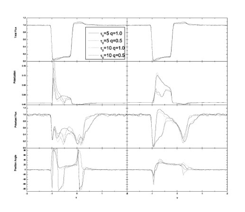
Figure 21: Similar to Fig. 17 but for LESR.

O99 detected PA rotations as large as $20^{\rm o}$$\sim 30$^o in BAL troughs of several BAL QSOs. Numerical calculations suggest that flows should extend to at least $\theta_{0}\simeq 30$^o in order to account for PA rotation larger than 15^o (see Table 2). The PA of polarization varies across the line profile in simulation, and its profile depends also strongly on the inclination and velocity distribution, but very weakly on the optical depth for the large $\tau_{0}$ models considered (Fig. 16 to Fig. 21). For a wide range of models, the maximum PA rotation occurs at a small velocity of the BAL trough at small inclinations, and at a large velocity at large inclinations. Thus, it may be used as an indicator of the inclination angle of the system. Indeed, both cases have been observed (O99).

The misalignment of the symmetric axes between the electron-scatterer and resonance scatterer can also lead to PA rotation. However, the physical driver for such misalignment is not clear. Furthermore, if the size of the electron-scatterer is small and the optical depth of the line is large, one would expect a constant PA rotation across the BAL trough, which seems not a general case for BAL QSOs, for non-rotating flows because the resonant scattered light dominates the polarization in the trough. A large electron scatterer can produce velocity-dependent PA rotation in the trough due to back-scatter effect as discussed in the §4.1 because the scattered photons from the reflection-symmetric sites will encounter the flow of different velocities on the way to the observer. The large electron scatterer will also produce a PA rotation without a jump at the start velocity of the trough, just same as the axisymmetric rotating outflow model with a LESR.

5.3 Polarized Flux and Sub-troughs

Several models predict distinct features, which reflect a special velocity field or geometry of the outflow. Some of these features are indeed observed in a number of BAL QSOs. Red sub-trough in the polarized flux is predicted by models of large $\theta_{0}$, and appears in the polarized spectra of several BAL QSOs such as 0105-265, 0226-1024, 1333+2840, 1413+1143 (O99). The observed sub-trough is usually narrower and shallower than the primary one (blue), in agreement with our simulations. There is also an emission like feature around $v=0$ (but no correspondent CIII] emission feature) in the polarized flux in some of these sources, such as 1413+1143. It should be noted that our model predicts large PA rotation for these objects in general (Table 2). Three out of four objects indeed show large PA rotations (-10^o for 0226-1024, 10^o for 1333+2840 and 20^o for 1413+1143). No apparent PA rotation in 0105-265 may be an indication of low angular-momentum outflow or a large optical depth to the resonant scattering in this object. The appearance of the sub-trough in the polarized flux is ascribed to the rotation of the STOKES $Q$ of the resonance scattering light (Appendix A) across the absorption line profile. Direct evidence for this comes from the polarization observation of 0043+0048: the continuum is not polarized but the BAL trough is; the Stokes parameters $Q$ is about 5% of the total intensity around the absorption trough, and changes its sign around zero velocity, similar to our numerical results with a large $\theta_{0}$.

Ogle (1997) proposed that the red sub-trough in 0226-1024 can be produced by polar an electron-scattering region with an equatorial BALR. To investigate the feasibility of this scenario, we carry out the simulation of resonant scattering for the case in which the incident continuum is polarized in the direction perpendicular to the symmetric axis of the resonant scatterer (PA${}_{c}=90$^o), as produced by a polar electron-scatterer. Models A0-12^o, A0-45^o, B0-33^o-20^o and B0-45^o-30^o are used in this simulation. The simulated polarized spectra are shown in Fig. 23. The polarization of the primary trough is indistinguishable from those with equatorial electron-scattering presented in §4.3 for all models considered. This is expected because the polarized flux in the trough is dominated by the resonantly scattered light for the range of optical depth concerned. However, the profile to the red side is very different for polar and equatorial scattering. These results are consistent with the analysis presented in Appendix A. For model A-12^o with PA${}_{c}=90^{\rm o}$, the polarized flux to the red side of the primary trough is also cancelled and the sub-trough is broader than and blending with the primary trough, which is not consistent with the observation. For model B there is a peak to the red side of the trough, which is not consistent with the observation too. Only in one case A0-45^o viewed in $i=90^{\rm o}-\theta_{0}$, there is a separated sub-trough to the red side of the primary trough, but the sub-trough is blue-shifted and a peak appears to the red side of it. So the model with large $\theta_{0}$ and PA${}_{c}=0$^o should be a better explanation for the sub-trough in 0226-1024 and other sources than that with PA${}_{c}=90^{\rm o}$(or polar electron scatterer).

Interestingly, 0932+5006 displays a polarized flux peak to red side of the primary trough which has no corresponding emission lines in the total flux. According to our analysis it can be produced by a polar electron scattering region plus an outflow with a geometry similar to the model B. But this is a rare case among the 36 sources in O99. It must be mentioned that if the electron scatterer covers the same sky as the BALR for model B-45^o-30^o, according to the $Eq.$ 7 and 8 of Paper I, the scattered light by electrons is polarized in the direction perpendicular to the axis of the scatterer. The polarized flux distribution to the red side of the trough is same as the result of model B-45^o-30^o plus a polar electron scatterer. So the source 0932+5006 can be interpreted by this model, as well.

Another characteristics in polarized flux is noted by Ogle that in some objects the troughs in polarized flux is more blueshifted than that in the total flux. In our models with LESR the starting velocity of the absorption in polarized flux is about $-v_{\varphi,0}$ (if $v_{\varphi,0}>v_{0}$) or $-v_{0}$ (if $v_{\varphi,0}<v_{0}$), if $v_{\varphi,0}>v_{0}$ it reproduces this characteristic. Model B with LESR might produce $\sim$90^o PA swing at velocity $v<-v_{\varphi,0}$ in our simulation, it is also found in several cases, for example 1212+1445 (CIV trough) and 1232+1325 (NV+Ly$\alpha$ trough). The two characteristics both indicate that the electron scattering region and the resonant scattering region are very close, or even coexist. Objects 1212+1445 and 1232+1325 are both low ionized BAL QSOs so the column of outflow is large and consistent with our results.

6 The Contribution of the Resonant scattered photons to the Broad Emission Line

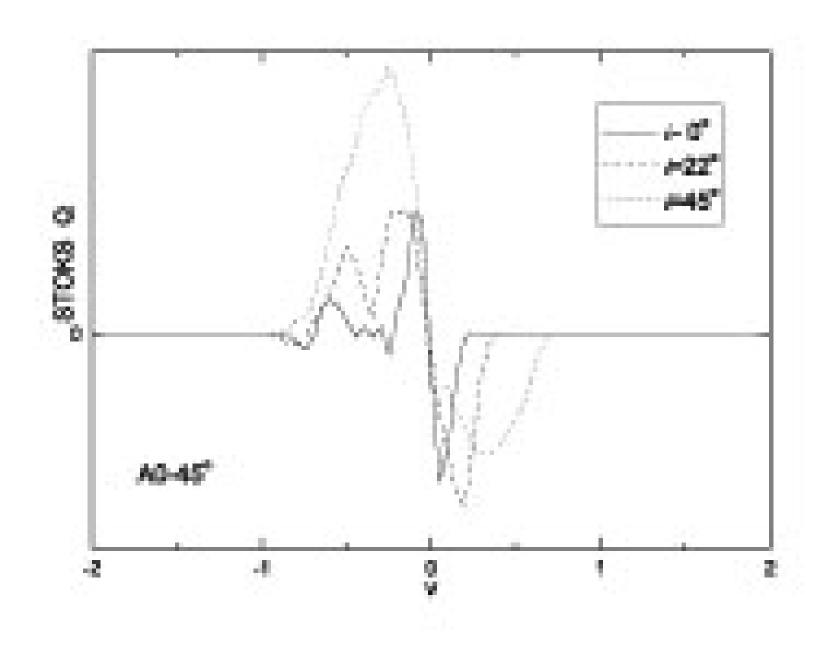
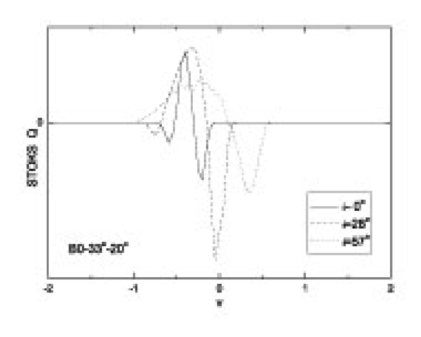
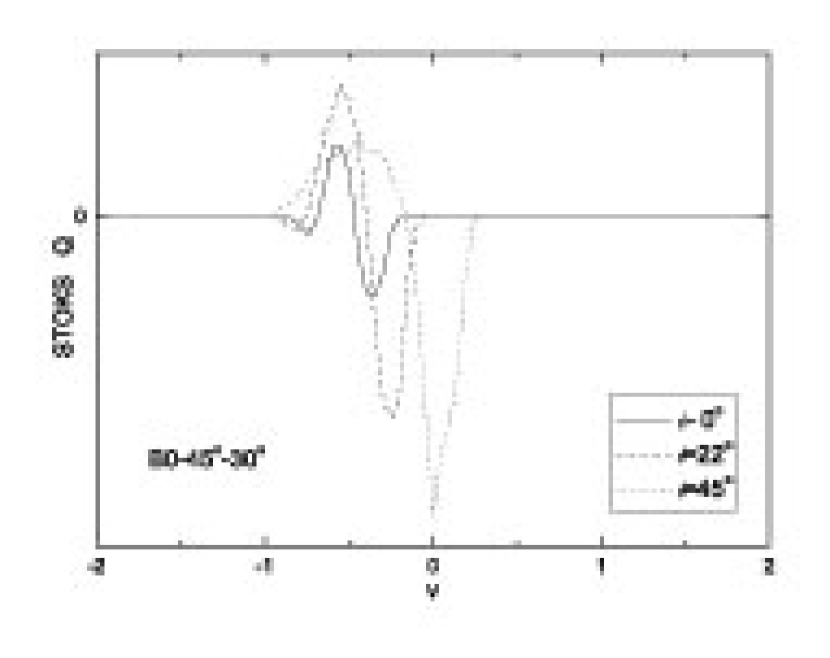
Figure 26: The simulated polarized flux, resonantly scattered by the BALR to different inclinations. Models of the BAL outflow are labelled in the figure and $\tau_{0}=5$.

Around half of the resonantly scattered photons in the BALR are absorbed by the accretion disk, and the rest emerge as emission line photons. If the BALR exists in all quasars, the contribution of the resonantly scattered photons to be observed emission lines might be non-negligible for non-BAL QSOs. In Fig. 26 we present the polarized flux resonantly scattered into the line of sight of non-BAL QSOs, which appears unique asymmetric, and thus may be used to test the presence of BALR in non-BAL QSOs.

Their contribution is especially important for NV emission line, which was used in the determination of the metal abundance in quasars (Hamann & Ferland 1992; 1993). HKM93 considered this problem in detail. Our treatment is different from theirs in serval aspects. First of all, we perform Monte-Carlo simulations to calculate the radiative transfer instead of using an escape probability approximation. Second, we consider a much larger range of the scattering optical depth in comparison with theirs, as required by observations. Third, we consider the rotation velocity of the flow and use a different radial velocity-law. Finally, we consider the absorption of the scattered photons by the accretion disk. In this section we mainly consider model A-12^o.

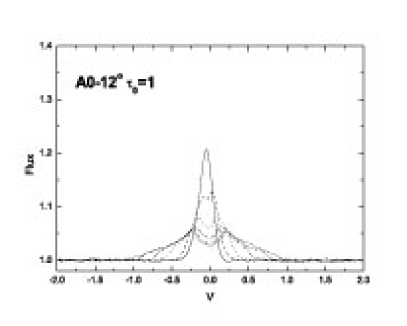
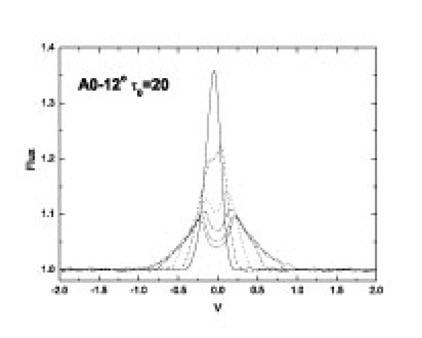
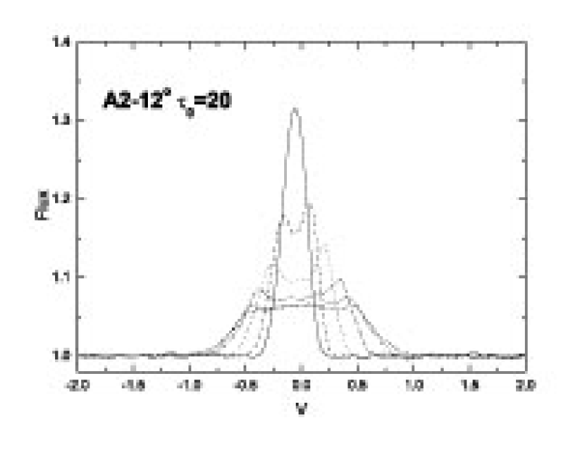
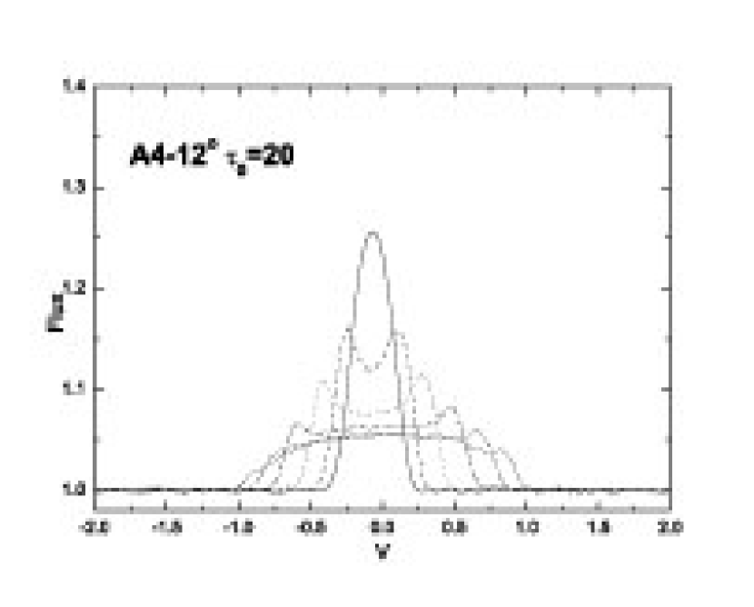
Figure 24: Scattered line profile (continuum has been normalized to unity) viewing at 6 different inclinations: $i\sim$ 0^o , 16^o , 27^o , 42^o , 58^o and 77^o for non-BAL QSOs. Parameters of the flows are: $\tau=1$ and $q=0.0$ in top-left panel, and $\tau=20$ and $q=0.0$ in the top-right panel, and $\tau=20$ and $q=0.5$ in bottom-right panel, $\tau=20$ and $q=1.0$ in the bottom-right panel.

For a pure radial outflow, the line profile of the scattering emission is qualitatively similar to that of HKM93 (Fig. 24, the upper two panels and figure 7, 8 of HKM93). Note due to the disk absorption, the contribution of the scattered photons only come from the facing half of the BALR, and the line profile is slightly blue-shifted relative to the HKM93 (Fig. 24). When the rotation is significant, the profiles are much different (Fig. 24, lower two panels): at intermediate inclinations the two peaks in the profile are further separated because the scattered photons preferably escape in the rotational direction, along which the velocity gradient is large; at high inclinations, the peaks disappear and the line profiles become flatter and the half width of the ”platform” is about $q\times v_{\infty}=v_{\varphi,0}$.

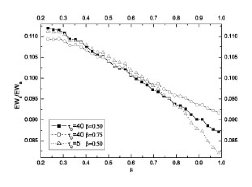
Figure 25: The equivalent width ratio of the scattering emission to the BAL for model A-12^o as a function of $\mu=\cos i$.

The scattering emission is stronger in the equatorial direction, at least for $\beta=0.5$ and $\beta=0.75$ (Fig. 25). For model A4-12^o with the $\tau_{0}=40$, we get a maximum EW (for non-BAL QSOs) of the scattering emission $w_{sl}$ which is about 11% of the corresponding BAL EW. The fraction increases to 18.6$\%$ for model A4-24^o. The scattering emission of NV 1240 is even stronger because of the scattering of the strong Ly$\alpha$ emission line. For example, in 0105-265 nearly half of Ly$\alpha$ emission line, of which the EW is $\approx 250$Å, is scattered by the NV ions (O99). According to the ratio noted above, the total EW of the scattering NV emission would be $(EW_{{\mathrm{L}y}\alpha}/2+EW_{BAL})\times 11\%=20.8$Å for A4-12^o, and 35.2Å for A4-24^o if the BAL extends to 2 $\times$ 10⁴ km s^-1. This is significant considering the observed EWs of NV emission line is only in the range of 9.2Å  to 44.8Å  (Ferland et al. 1996). Therefore, a strong NV may not indicate a high metal abundance but a large covering factor of the BALR. If this is indeed the case, we also expect that the EW of NV$\lambda$1240 be correlated with continuum polarization.

HKM93 used $W_{\lambda}(em)/W_{\lambda}(abs)$ of the BAL QSOs to set an upper limit of the covering factor, about 0.2. Here we point out that if the disk absorption is considered, the upper limit should bounce up to 0.4. Following HKM93’s calculation (their $Eq.$ 1), we estimate the effective ”covering factor” from the simulated total flux spectrum for each model. As expected, we find that the effective ”covering factor” (using $Eq.$ 1 of HKM93) is about half the solid angle subtending by BALR. For the models in the previous section, we obtained a ”covering factor” of 0.34$\sim$0.40 for model A0-45^o, 0.26$\sim$0.28 for model A0-30^o, 0.115 for model A0-12^o, 0.06$\sim$0.08 for model B0-45^o-30^o and 0.10 for model B0-33^o-20^o.

Note in passing, polarization observations of resonant lines in non-BAL quasars should provide a good test to the unification model of BAL and non-BAL. The polarization of the scattering lines show unique profile across the line profile, and depends strongly on the inclinations and model parameters (Fig 26). In particular, the subtending angle of the flows is also directly relative to amount of scattering light, thus the polarization degree. The observations would be preferably to be done for NV-strong quasars if the interpretation of strong NV emission as due to resonance scattering is correct. Thus the observation, in turn, provides a check for the scenario.

7 Summary

Polarization provides rich information on the structure and kinematics of BALR in QSOs, which is complementary to those derived from absorption lines, which only depend on the physical condition and kinematics of gas on the LOS. To extract this information, we carry out extensive Monte-Carlo simulations of electron and resonance scattering process in the BALRs. Both singlet and doublet transitions are considered for radial outflows of two different geometries: equatorial outflows and hollow-conical outflows with and without rotational velocities.

In an axisymmetric scatterer model, PA rotation in the absorption trough can be produced only when the outflow carries angular momentum. The PA rotation increases with the angular velocity as well as the subtending angle of the flow. In order to produce a PA rotation $>$ 10^o observed in a few BAL QSOs, subtending angle of the outflow should be larger than 25^o . Similar requirement is imposed to explain the red sub-trough in the polarized flux observed in some BAL QSOs.

Resonant scattering of doublet transition produces much lower polarization at large optical depths (about 6% for $\tau_{0}=5$, $\beta=0.5$) for an accelerating outflow. Large ($>$10%) polarization in the absorption trough detected in a few BAL QSOs may indicate that the optical depth to the resonant scattering is at most moderate, otherwise resonant scattering of $T_{1/2}$ transition will erase all polarization. A slowly-accelerating model can produce larger polarization. If the observed high-velocity outflow in X-ray is real, the flow is likely decelerating, which will produce much larger polarization.

A large electron scattering region can also produce larger polarization. The jump which appears at the starting velocity of the absorption trough in PA rotation and polarized flux in models with a SESR does not appear in the model with a LESR. This characteristic may be an important indicator to distinguish different electron scattering models. We find that LESR models can explain that the absorption troughs are more blueshifted in polarized flux, relative to that in the total flux, and PA swings in the troughs, $\sim 90^{\rm o}$ relative to continuum, in some objects.

We show that the resonantly scattered light will contribute a significant part of NV in some QSOs and can give rise to anomalous strong NV lines in these QSOs. A correlation between the EW of NV$\lambda$1240 with the continuum polarization is expected. We propose that the polarized flux and the PA rotation of the scattering emission can be used to test the presence of BALR in non-BAL QSOs. Further observations with large telescopes should allow us to extract the important information about the flow geometry and kinematics.

Appendix A: Notes on the red-trough in the polarized flux

We denote the Stokes parameters $Q$ and $U$ of the continuum as $Q_{c}$ and $U_{c}$. For simplicity, we choose $U_{c}=0$ and $|Q_{c}|=I^{c}_{pl}$, where $I^{c}_{pl}$ is the polarized flux of the continuum. If $Q_{c}>0$ the PA of the continuum polarization (hereafter $\mathrm{PA}_{c}$) is 0^o otherwise $\mathrm{PA}_{c}=90$^o. We assume that PA of the line scattered photon is PA_l so the $U_{l}=Q_{l}\tan($2PA${}_{l})$. The Stokes parameters of the total flux are $Q_{T}=Q_{c}+Q_{l}$, $U_{T}=U_{c}+U_{l}$; the total polarized flux $I^{T}_{pl}$ reads,

$$I^{T}_{pl}=\sqrt{U_{T}^{2}+Q_{T}^{2}}=\sqrt{Q_{l}^{2}(1+\tan^{2}(2\rm{PA}_{l}))+Q_{c}^{2}+2Q_{c}Q_{l}}$$ (1)

From this equation we find that $I^{T}_{pl}<I^{c}_{pl}$ if

$$\left\{\begin{array}[]{ll}0>Q_{l}>-\frac{2Q_{c}}{1+\tan^{2}(2\rm{PA}_{l})}&(\mathrm{PA}_{c}=0^{\rm o})\\ 0<Q_{l}<-\frac{2Q_{c}}{1+\tan^{2}(2\rm{PA}_{l})}&(\mathrm{PA}_{c}=90^{\rm o})\end{array}\right.$$

When $Q_{l}\times Q_{c}<0$ and $|Q_{l}|\lesssim|Q_{c}|$, one obtains $I^{T}_{pl}<I^{c}_{pl}$, i.e, an absorption trough appears in the polarized flux. Since the total flux equals to the $I_{c}+I_{l}>I_{c}$ the feature is not shown in the total flux. On the other hand, if $Q_{l}\times Q_{c}>0$, one yields $I^{T}_{pl}>I^{c}_{pl}$. In the rest of this appendix we will obtain the relationship between $Q_{l}$ and $Q_{c}$ for different models.

For simplicity, we consider single-scattering of the unpolarized incident spectrum by singlet transition. The density matrix of the incident continuum is

$$\rho^{i}_{11}=\rho^{i}_{22}=1/2;\rho^{i}_{12}=\rho^{i}_{21}=0$$ (2)

Now consider an outflow between [90${}^{\rm o}-(\theta_{0}-d\theta_{0})$, 90^o$-\theta_{0}$]. For light from an incident direction $(\theta_{i},\varphi_{i})$ that is scattered into the direction $(\theta_{o},\varphi_{o})$, the density matrix can be written as (see $Eq.$ 1 & 2 of Paper I):

$$\rho^{o}_{11}\propto\frac{1}{2}[\sin^{2}\theta_{0}\cos(\varphi_{i}-\varphi_{o})+\cos^{2}\theta_{0}]^{2}+\frac{1}{2}\sin^{2}\theta_{0}\sin^{2}(\varphi_{i}-\varphi_{o})$$ (3)

$$\rho^{o}_{22}\propto\frac{1}{2}\sin^{2}\theta_{0}\sin^{2}(\varphi_{i}-\varphi_{o})+\frac{1}{2}\cos^{2}(\varphi_{i}-\varphi_{o})$$ (4)

The Stokes parameter $Q$ of the scattered light reads

$$Q_{l}(\varphi_{i},\varphi_{o})=\rho^{o}_{11}-\rho^{o}_{22}\propto\frac{1}{2}[\sin^{2}\theta_{0}\cos(\varphi_{i}-\varphi_{o})+\cos^{2}\theta_{0}]^{2}-\frac{1}{2}\cos^{2}(\varphi_{i}-\varphi_{o})$$ (5)

It is easy to prove

$$Q_{l}\geq 0\;\;{\mathrm{f}or}\;\;-90^{\rm o}<\varphi_{i}-\varphi_{o}<90^{\rm o}$$ (6)

and $Q_{l}<0$, when

$$180^{\rm o}+\csc\frac{1-\sin^{2}\theta_{0}}{1+\sin^{2}\theta_{0}}>\varphi_{i}-\varphi_{o}>180^{\rm o}-\csc\frac{1-\sin^{2}\theta_{0}}{1+\sin^{2}\theta_{0}}$$ (7)

In an outflow model, red-shifted photons are escaped from the portion with 90${}^{\rm o}<\varphi_{i}-\varphi_{o}<270^{\rm o}$ and the blue-shifted ones from the -90${}^{\rm o}<\varphi_{i}-\varphi_{o}<90^{\rm o}$. According to $Eq.$ A6, the blue-shifted photons always have $Q_{l}\geq 0$. However, the redshifted scattered light may have negative $Q_{l}$ following $Eq.$ A7. The portion of the flow that produces negative $Q_{l}$ increases with $\theta_{0}$. It is small for small $\theta_{0}$ and reachs half of backward flow (135${}^{\mathrm{o}}<\varphi_{i}-\varphi_{o}<225^{\mathrm{o}}$) for $\theta_{0}\sim 25^{\mathrm{o}}$. Consequently, for a small $\theta_{0}$ the total $Q_{l}$ of red-shifted scattered photons is larger than 0. If $Q_{c}$ is also positive, an excess polarized flux across the emission line will be seen; otherwise, an absorption trough is observed (Fig. 22). For a large $\theta_{0}$, redshifted scattered light has negative $Q_{l}$, a sub-trough to the red side of primary trough will be observed when $Q_{c}$ is positive.

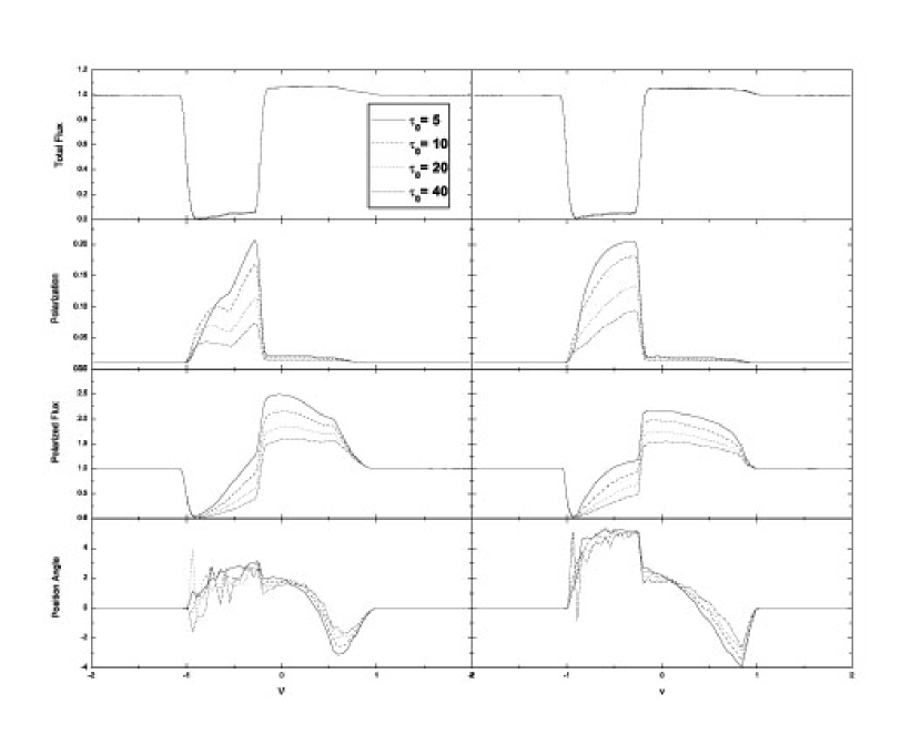
Figure 5: Similar to Fig. 4 but for model A2-12^o(left panel) and A4-12^o(right panel), in which flow has a rotational velocity. Rotational of flow produces a jump in the polarization at around $qv_{\infty}$ and PA rotation.

Figure 8: The total flux, polarization degree, polarized flux and the PA for singlet in the velocity space for model A-12^o and a large electron-scattering region(LESR) on the base of the outflow. In the left panel, $q=1.0$ and different $\tau_{0}$ is marked. In the right panel $\tau_{0}=10$ and different $q$ are marked.

Figure 13: The polarization degree, polarized flux and PA in the velocity space for WCRS, singlet and doublets model. The model adopted is model B4-45^o-30^o and a LESR, viewing from $i=45^{\rm o}$(left panel) and viewing from $i=60^{\rm o}$(right panel), assuming $\tau_{0}=10$.

References

- Antonucci (1993) Antonucci, R. 1993, ARA&A, 31, 473
- Arav et al. (1999) Arav, N., Becker, R. H., Laurent-Muehleisen, S. A., Gregg, M. D., White, R. L., Brotherton, M. S., & de Kool, M. 1999, ApJ, 524, 566
- Blandford et al. (2002) Blandford, R., Agol, E., Broderick, A., Heyl, J., Koopmans, L., & Lee, H. 2002, Astrophysical Spectropolarimetry, 177
- Blandford & Payne (1982) Blandford, R. D., & Payne, D. G. 1982, MNRAS, 199, 883
- Brinkmann et al. (1999) Brinkmann, W., Wang, T., Matsuoka, M., & Yuan, W. 1999, A&A, 345, 43
- Boroson (2002) Boroson, T. A. 2002, ApJ, 565, 78
- Chandrasekhar (1950) Chandrasekhar S., 1950, Radiative Transfer
- Chartas et al. (2002) Chartas, G., Brandt, W. N., Gallagher, S. C., & Garmire, G. P. 2002, ApJ, 579, 169
- Chartas et al. (2003) Chartas, G., Brandt, W. N., & Gallagher, S. C. 2003, ApJ, 595, 85
- Clavel et al. (2006) Clavel, J., Schartel, N., & Tomas, L. 2006, A&A, 446, 439
- Cohen et al. (1995) Cohen, M. H., Ogle, P. M., Tran, H. D., Vermeulen, R. C., Miller, J. S., Goodrich, R. W., & Martel, A. R. 1995, ApJ, 448, L77
- de Kool & Begelman (1995) de Kool, M., & Begelman, M. C. 1995, ApJ, 455, 448
- Dong et al. (2005) Dong, X.-B., Zhou, H.-Y., Wang, T.-G., Wang, J.-X., Li, C., & Zhou, Y.-Y. 2005, ApJ, 620, 629
- Elvis (2000) Elvis, M. 2000, ApJ, 545, 63
- Everett (2002) Everett J.E., 2002, submitted to ApJ
- Ferland et al. (1996) Ferland G.J., Baldwin J.A., Korista K.T., Hamann F., Carswell R.F., Phillips M., Wilkes B., Williams R.E., 1996, ApJ, 461, 683-697
- Gallagher, Brandt, Chartas, & Garmire (2002) Gallagher, S. C., Brandt, W. N., Chartas, G., & Garmire, G. P. 2002, ApJ, 567, 37
- Goodrich & Miller (1995) Goodrich, R. W., & Miller, J. S. 1995, ApJ, 448, L73
- Green et al. (2001) Green, P. J., Aldcroft, T. L., Mathur, S., Wilkes, B. J., & Elvis, M. 2001, ApJ, 558, 109
- Hamann (1998) Hamann F. 1998, ApJ, 500, 798
- Hamann & Ferland (1992) Hamann, F., & Ferland, G. 1992, ApJ, 391, L53
- Hamann & Ferland (1993) Hamann, F., & Ferland, G. 1993, ApJ, 418, 11
- Hamann, Korista, & Morris (1993) Hamann, F., Korista, K. T., & Morris, S. L. 1993, ApJ, 415, 541
- Hines & Wills (1995) Hines, D. C., & Wills, B. J. 1995, ApJ, 448, L69
- Hines et al. (1995) Hines, D., Schmidt, G., Smith, P., & Weymann, R. 1995, Bulletin of the American Astronomical Society, 27, 1410
- Hutsemkers & Lamy (2001) Hutsemkers D., Lamy H., 2001, ASP Conference Series
- Konigl & Kartje (1994) Konigl, A., & Kartje, J. F. 1994, ApJ, 434, 446
- Lamy & Hutsemékers (2004) Lamy, H., & Hutsemékers, D. 2004, A&A, 427, 107
- Lee, Blandford & Western (1994) Lee H.W., Blandford R.D., Western L., 1994, MNRAS267, 303-311
- Lee (1994) Lee H.W., 1994, MNRAS268,49-60
- Lee & Blandford (1997) Lee H.W., Blandford R.D., 1997,MNRAS, 288,19-42
- Martínez-Sansigre et al. (2005) Martínez-Sansigre, A., Rawlings, S., Lacy, M., Fadda, D., Marleau, F. R., Simpson, C., Willott, C. J., & Jarvis, M. J. 2005, Nature, 436, 666
- Murray et al. (1995) Murray N., Chiang J. Grossman S.A., Voit G.M., 1995, ApJ, 451, 498-509
- Ogle (1997) Ogle, P. M. 1997, ASP Conf. Ser. 128: Mass Ejection from Active Galactic Nuclei, 128, 78
- Ogle et al. (1999) Ogle P.M., Cohen M.H., Miller J.S., Tran H.D., Goodrich R.M., Martel A.R., 1999, ApJS. 125, 1-34
- Proga et al. (2000) Proga, D., Stone, J. M., & Kallman, T. R. 2000, ApJ, 543, 686
- Reichard et al. (2003) Reichard, T. A., et al. 2003, AJ, 126, 2594
- Ruiz et al. (2001) Ruiz, J. R., Crenshaw, D. M., Kraemer, S. B., Bower, G. A., Gull, T. R., Hutchings, J. B., Kaiser, M. E., & Weistrop, D. 2001, AJ, 122, 2961
- Schmidt & Hines (1999) Schmidt, G. D. & Hines, D. C. 1999, ApJ, 512, 125
- Stockman, Moore, & Angel (1984) Stockman, H. S., Moore, R. L., & Angel, J. R. P. 1984, ApJ, 279, 485
- Voit, Weymann, & Korista (1993) Voit, G. M., Weymann, R. J., & Korista, K. T. 1993, ApJ, 413, 95
- Wang et al. (2005) Wang, H.-Y., Wang, T.-G., & Wang, J.-X. 2005, ApJ, 634, 149
- Wang et al. (2000) Wang, T. G., Brinkmann, W., Yuan, W., Wang, J. X., & Zhou, Y. Y. 2000, ApJ, 545, 77
- (44) Wang T.G., Wang J.X., Brinkmann W., Matsuoka M., 1999, ApJL. 519, L35-L38
- Weymann et al. (1991) Weymann R.J., Morris S.L., Foltz C.C., Hewett P.C., 1991, ApJ, 373, 23
- Zhou et al. (2006) Zhou, H., Wang, T., Wang, H., Wang, J., Yuan, W., & Lu, Y. 2006, ApJ, 639, 716