Orientation effects in Bipolar nebulae

Abstract

We show that the inclination to the line of sight of bipolar nebulae strongly affects some of their observed properties. We model these objects as having a spherically symmetric Planetary Nebula and a dusty equatorial density enhancement that produces extinction that varies with the viewing angle. Our sample of 29 nebulae taken from the literature shows a clear correlation between the inclination angle and the near-IR and optical photometric properties as well as the apparent luminosity of the objects. As the inclination angle increases –the viewing angle is closer to the equatorial plane– the objects become redder, their average apparent luminosity decreases, and their average projected expansion velocity becomes smaller.

We compute two-dimensional models of stars embedded in dusty disks of various shapes and compositions and show that the observed data can be reproduced by disk-star combinations with reasonable parameters. To compare with the observational data, we generate sets of model data by randomly varying the star and disk parameters within a physically meaningful range.

We conclude that a only a smooth pole to equator density gradient agrees with the observed phenomena and that thin, equatorially concentrated disks can be discarded.

1 Introduction

Planetary Nebulae (PNe) and Symbiotic Nebulae are the visible remains of a heavy mass loss period near the end of the lives of most low and intermediate mass stars (Gurzadyan (1997)). A fraction of PNe is bipolar (BPNe) and this morphology is likely caused by having a binary for central star (Soker (2004)). BPNe have special properties (Corradi & Schwarz (1995)) and are important objects for the study of outflows, mass loss, and binarity in PNe Several meetings have been dedicated to asymmetrical PNe (Harpaz, Soker (1995), Kastner, Soker, Rappaport (2000), Meixner, Kastner, Balick, Soker (2004)), see references herein.

The orientation angle on the plane of the sky of asymmetrical PNe has been studied more than 30 years ago by Melnick & Harwit (1975) and more recently by Phillips (1997) who both found an apparent alignment of the long axes of PNe with the plane of the Galaxy. The paper by Corradi et al. (1998) –based on a larger sample and using more rigorous statistical methods– showed that there is no significant alignment and that PNe are essentially randomly distributed on the sky. Assuming that this random distribution also holds for the inclination with respect to the line of sight –where the inclination, i, is taken to be 0^o for a pole-on nebula and 90^o for an object viewed with its main axis parallel to the plane of the sky–we investigate the possible effects of orientation on the observational properties PNe.

Su, Hrivnak, Kwok (2001) studied the observational orientation effects in six bipolar Proto-PNe and found that objects are redder when viewed edge-on i.e. have the inclination angle i near 90^o, as expected from simple geometrical extinction considerations nd assuming some equatorial density enhancement. From these data they concluded that Proto-PNe generally have bipolar shapes and asymmetrical dust disks.

Here we present a more general look at the phenomenon and apply a simple model to a larger sample of objects that we know to be bipolar, to see if we observe differences as a function of inclination angle. We study a range of overall geometries and dust properties of the equatorial tori, different black-body temperature ratios between the dust and central stars, and simulate observational data sets by letting these model parameters vary randomly over a restricted and physically meaningful range. These data sets we then compare directly with our observed results.

2 Observational material

We have collected a sample of 29 bipolar planetary nebulae and symbiotic nebulae that had sufficient data available in the literature to construct a reasonable spectral energy distribution (SED), with at least some data points in the optical, near-IR, and mid-IR wavelength ranges. Table 1 lists our sample of objects and their calculated relative luminosities in each of the three bands that we defined as follows.

Table 1: Our observed sample of BPNe. Listed are: PK name, common name, B, V, R, J, H, and K in magnitudes; 12, 25, 60, 100 fluxes in Janskys, the inclination angle (i) in degrees, and the apparent luminosity (L) in W.m² scaled as the square of the distance as derived from the SED.

Name	B	V	R	J	H	K	12	25	60	100	i	L
19W32	18.2	17.2	14.3	10.8	9.3	8.6	3.4	12.6	23.0	356.0	80.	1.99244e-12
Hb5	10.3	8.2	-	9.5	8.8	8.6	11.68	79.24	134.50	311.8	65.	1.39518e-11
He2-25	16.4	-	13.9	10.7	9.7	9.5	0.742	2.11	3.39	41.0	90.	5.23481e-13
He2-36	11.9	11.2	8.9	9.8	9.6	9.4	0.42	4.88	6.40	8.8	30.	1.67762e-12
He2-111	16.3	16.7	-	13.5	11.1	9.7	1.28	3.08	11.21	117.2	70.	7.42040e-13
He2-114	18.7	-	16.3	-	-	-	2.0	0.38	3.08	38.46	45.	3.06317e-13
He2-145	19.1	-	16.4	12.0	10.9	10.1	3.1	2.67	44.75	201.0	55.	2.21225e-12
IC4406	12.7	-	11.4	-	-	10.1	0.33	2.69	21.08	25.35	65.	1.18293e-12
07131-0147	15.4	-	11.7	10.2	9.5	9.1	2.59	4.22	3.96	3.68	60.	8.54946e-13
K3-46	19.1	-	16.3	13.8	13.0	12.7	0.7	0.25	0.73	5.87	65.	1.04686e-13
M1-8	11.7	-	10.4	10.7	10.5	9.8	0.25	0.66	3.10	5.54	25.	7.55110e-13
M1-13	11.0	-	9.9	-	-	-	0.25	0.70	4.51	9.37	25.	4.58175e-12
M1-16	12.7	-	10.0	13.0	13.2	12.2	0.32	2.33	9.45	7.59	60.	7.58743e-13
M1-28	18.9	-	16.0	15.1	14.2	13.8	2.4	0.41	2.77	11.75	55.	3.11362e-13
M1-91	16.3	15.0	12.4	-	-	-	3.85	8.29	12.14	9.56	75.	1.26640e-12
M2-9	11.3	-	9.5	10.9	9.2	7.0	50.50	110.20	123.60	75.84	75.	1.19351e-11
M2-48	15.2	-	10.0	15.9	14.4	13.9	1.03	0.76	7.42	35.86	45.	7.52791e-13
M3-28	15.6	-	10.3	-	9.6	8.0	3.53	2.56	46.94	320.60	60.	3.16344e-12
MyCn18	11.8	-	9.6	11.8	10.3	9.8	1.80	20.66	24.28	13.24	55.	2.17540e-12
Mz1	12.8	-	11.6	-	-	-	0.48	1.40	14.45	92.96	50.	1.57525e-12
Mz3	10.8	-	8.0	9.2	7.4	5.6	88.76	343.20	277.00	112.60	65.	3.00787e-11
NGC650-51	-	17.7	-	16.0	15.9	15.6	0.28	2.79	6.80	9.29	60.	3.09241e-13
NGC2346	11.5	11.2	-	10.2	9.4	8.4	0.47	0.88	7.97	13.40	45.	1.15817e-12
NGC2440	11.8	-	11.0	10.6	10.8	10.1	3.59	28.01	43.47	26.30	65.	2.64962e-12
NGC2818	16.8	-	16.8	-	-	18.2	0.32	1.00	2.30	2.89	90.	1.25058e-13
NGC2899	17.8	-	16.3	-	-	-	0.27	1.42	5.13	10.91	75.	2.59349e-13
NGC6072	11.6	-	10.1	-	-	-	0.38	2.87	24.89	31.17	45.	4.33377e-12
NGC6302	-	9.1	7.1	9.5	9.7	8.6	32.08	335.90	849.70	537.40	70.	3.66894e-11
NGC6445	11.6	-	12.5	10.9	9.6	9.2	1.50	15.01	44.44	43.23	50.	2.22741e-12
NGC6537	11.0	-	12.0	10.3	10.4	9.3	7.72	58.30	189.90	166.10	60.	7.70877e-12
NGC7026	15.3	14.2	11.7	10.2	11.0	9.6	2.39	18.35	42.74	30.91	50.	2.03701e-12
Na2	18.7	-	-	15.9	15.7	14.6	0.46	0.33	0.93	1.32	-	7.45171e-14
Sa2-237	16.1	15.5	15.0	13.1	12.6	11.8	1.17	6.01	16.56	8.29	70.	6.57414e-13
SH1-89	15.8	-	13.6	14.4	13.2	12.8	0.89	0.25	2.14	20.15	-	1.88058e-13
TH2-B	19.4	-	16.7	-	-	-	1.40	2.15	3.22	34.68	-	3.24659e-13
He2-104	13.5	14.6	11.1	10.8	8.9	7.0	8.56	9.09	6.83	9.77	50.	2.14718e-12
BI Cru	12.5	10.9	11.3	7.3	6.0	4.8	17.29	15.34	11.84	119.10	40.	1.20309e-11
R Aqr	10.0	6.2	-	0.5	-0.1	-0.8	1577.0	543.80	66.65	16.60	20.	2.83343e-09
AS201	12.4	12.5	11.3	10.6	10.2	9.5	4.12	38.33	76.14	41.49	-	3.59771e-12

After constructing the SEDs we defined three different apparent luminosities: visible (BVR), NIR (JHK) and IRAS (12, 25, 60, & 100 $\mu$m) and divided these three luminosities by the total (near-bolometric) apparent luminosity as derived from the SED. All luminosities were calculated by integrating the F($\lambda$) curve over the appropriate wavelength range. Possible differences in the line of sight interstellar extinctions were ignored. These differences would affect mainly the BVR luminosity since the extinction is a strongly declining function of wavelength. For those objects that could have their absolute luminosity determined, we also investigated the dependence of the absolute luminosity on the inclination angle. There were only 7 objects with good enough distances for computing an believable absolute luminosity.

The last column in Table 1 shows the average of the three estimated inclination angles for each object. The inclination angles were determined by the three authors independently, to obtain an idea of the associated uncertainties in deriving inclinations from optical images. The process has a subjective component but we found (somewhat to our surprise!) that for nearly all cases our independent estimates were in agreement to within 10 ^o or so, accurate enough for the purposes of this paper. For only three “recalcitrant” objects did we differ by as many as 30 ^o in our estimates.Typical standard deviations of the mean of the three estimates are 5-8 ^o and in all cases they were below 18 ^o.

In Figure 1 we plot the relative luminosities for each band –visible (BVR); NIR (JHK); MIR (IRAS bands)– as a function of the inclination angle. One can clearly see the increase of relative MIR as well as the decrease of JHK and BVR with increasing inclination for the sample.

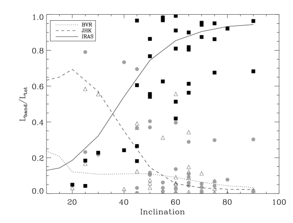
Figure 1: The observed relative luminosities in the BVR (open triangles), JHK (grey dots), and IRAS (black squares) bands as a function of the inclination angle. The best fitting model is overplotted as lines (solid = IRAS; dashed = JHK; dotted = BVR).

Table 2: Apparent total, BVR, JHL, and IRAS luminosities and inclinations for objects studied. See text for the detailed definition of these luminosities.

PK	Name	BVR	JHK	IRAS	$L_{Total}$	Incl.
-	07131-0147	$5.65\times 10^{-5}$	$5.64\times 10^{-2}$	$2.65\times 10^{-1}$	$6.78\times 10^{-1}$	60
359.2+01.2	19W32	$1.81\times 10^{-4}$	$1.08\times 10^{-3}$	$9.48\times 10^{-2}$	$9.04\times 10^{-1}$	80
-	BI Cru	$8.51\times 10^{-4}$	$1.61\times 10^{-2}$	$7.35\times 10^{-1}$	$2.49\times 10^{-1}$	40
359.3-00.9	Hb5	$7.45\times 10^{-4}$	$1.70\times 10^{-1}$	$4.70\times 10^{-2}$	$7.83\times 10^{-1}$	65
004.8+02.0	He2-25	$5.99\times 10^{-5}$	$9.33\times 10^{-3}$	$2.34\times 10^{-1}$	$7.57\times 10^{-1}$	90
359.6-04.8	He2-36	$1.14\times 10^{-4}$	$4.10\times 10^{-1}$	$1.88\times 10^{-1}$	$4.01\times 10^{-1}$	30
315.4+09.4	He2-104	$2.05\times 10^{-4}$	$2.33\times 10^{-2}$	$5.07\times 10^{-1}$	$4.70\times 10^{-1}$	50
315.0-00.3	He2-111	$5.64\times 10^{-5}$	$1.22\times 10^{-3}$	$5.83\times 10^{-2}$	$9.40\times 10^{-1}$	70
318.3-02.0	He2-114	$2.49\times 10^{-5}$	$1.75\times 10^{-3}$	$2.53\times 10^{-2}$	$9.73\times 10^{-1}$	45
331.4+00.5	He2-145	$1.14\times 10^{-4}$	$4.13\times 10^{-4}$	$3.24\times 10^{-2}$	$9.67\times 10^{-1}$	55
319.6+15.7	IC4406	$5.12\times 10^{-5}$	$9.05\times 10^{-2}$	$9.98\times 10^{-2}$	$8.10\times 10^{-1}$	65
069.2+03.8	K3-46	$8.12\times 10^{-6}$	$6.44\times 10^{-3}$	$7.91\times 10^{-2}$	$9.14\times 10^{-1}$	65
210.3+01.9	M1-8	$4.13\times 10^{-5}$	$3.93\times 10^{-1}$	$3.30\times 10^{-1}$	$2.77\times 10^{-1}$	25
232.4-01.8	M1-13	$6.57\times 10^{-5}$	$4.07\times 10^{-1}$	$3.68\times 10^{-1}$	$2.25\times 10^{-1}$	25
226.7+05.6	M1-16	$6.01\times 10^{-5}$	$3.22\times 10^{-1}$	$1.01\times 10^{-1}$	$5.77\times 10^{-1}$	60
0.060+03.1	M1-28	$2.11\times 10^{-5}$	$2.91\times 10^{-3}$	$3.11\times 10^{-2}$	$9.66\times 10^{-1}$	55
-	M1-91	$8.78\times 10^{-5}$	$1.62\times 10^{-2}$	$7.41\times 10^{-2}$	$9.10\times 10^{-1}$	75
010.8+18.0	M2-9	$1.28\times 10^{-3}$	$2.43\times 10^{-2}$	$2.02\times 10^{-1}$	$7.74\times 10^{-1}$	75
062.4-00.2	M2-48	$5.02\times 10^{-5}$	$3.04\times 10^{-1}$	$2.68\times 10^{-2}$	$6.69\times 10^{-1}$	45
021.8-00.4	M3-28	$1.87\times 10^{-4}$	$4.40\times 10^{-2}$	$1.30\times 10^{-1}$	$8.26\times 10^{-1}$	60
307.5-04.9	MyCn18	$1.58\times 10^{-4}$	$1.42\times 10^{-1}$	$4.47\times 10^{-2}$	$8.13\times 10^{-1}$	55
322.4-02.6	Mz1	$5.12\times 10^{-5}$	$7.30\times 10^{-2}$	$7.18\times 10^{-2}$	$8.55\times 10^{-1}$	50
331.7-01.0	Mz3	$2.90\times 10^{-3}$	$3.29\times 10^{-2}$	$1.68\times 10^{-1}$	$7.99\times 10^{-1}$	65
130.9-10.5	NGC650-51	$1.32\times 10^{-4}$	$2.11\times 10^{-4}$	$5.84\times 10^{-1}$	$4.16\times 10^{-1}$	60
215.6+03.6	NGC2346	$6.03\times 10^{-5}$	$2.07\times 10^{-1}$	$4.22\times 10^{-1}$	$3.71\times 10^{-1}$	45
234.8+02.4	NGC2440	$2.28\times 10^{-4}$	$4.24\times 10^{-2}$	$7.88\times 10^{-2}$	$8.79\times 10^{-1}$	50
-	R Aqr	$7.10\times 10^{-2}$	$3.67\times 10^{-2}$	$8.01\times 10^{-1}$	$1.62\times 10^{-1}$	20
011.1+07.0	Sa2-237	$3.00\times 10^{-4}$	$7.30\times 10^{-3}$	$1.80\times 10^{-2}$	$9.60\times 10^{-1}$	70

The observed relative luminosities in the BVR, JHK, and IRAS bands are shown as a function of inclination angle in Figure 1.

3 Models

3.1 A simplified 2-D radiative transfer code

To try to explain this observed behavior, we propose that these bipolar systems are composed of a dusty equatorial density enhancement being irradiated by a star or a binary system. The UV flux from this system heats up the dust that then re-emits the radiation in the IR. The combined effect of this re-radiation with the extinction produced by the density distribution is what produces the observed effect.

To simulate this system we created a simple 2-D radiative transfer code using the IDL package. This code works by creating a 2-D grid of cells, each having a given density. By requiring conservation of luminosity at each cell and iterating we determine the temperature of the dust. The temperature is determined from the following equation:

$\int C_{abs}cu_{\lambda}d\lambda=\int C_{abs}4\pi B_{\lambda}(T)d\lambda$

where T is the temperature, $u_{\lambda}$ is the energy density of the radiation field and $C_{abs}$ is the absorption cross-section, shown in Figure 2 as a function of the wavelength. Secondary radiation is as of yet not accounted for. Scattering is calculated assuming an isotropic phase function.

Some simplifying assumptions are made concerning the dust grains:

1. the dust species are well mixed, allowing for the use of average cross-sections;

2. the dust mixture is in equilibrium with the radiation field which implies a single dust temperature for all dust species;

3. the dust-to-gas ratio is the same as the one for the interstellar medium.

For the dust characteristics we then adopted typical interstellar grains with R_v = 3.1 and absorption cross-section calculated by Li & Draine (2001) with a dust to gas ratio of 0.008. The absorption cross-section is shown in Figure 2.

Figure 2: Absorption cross-sections used in the model calculations. From Li & Draine (2001).

With the 2-D temperature and density grids, we constructed a 3-D grid where the calculated intensity emitted by the dust plus scattered radiation (assumed isotropic) is obtained for each cell. Using this cube and the extinction cross-section from Li & Draine (2001) we calculated the image projected onto the sky for a given line of sight. The total emitted radiation was obtained from this projected image and was then compared to observational results.

3.2 Calculated Models

Using the simple code described above we initially calculated models for the three basic disk-like structures shown in Figure 3, 1st column. From top to bottom these are: a) a torus; b) a flat disk and c) a curved disk. A fourth distribution was used with a much more smoothly varying density gradient from pole to equator, shown as the last entry in the 1st column of Figure 3. For simplicity we adopted the same physical size and peak density for all structures.

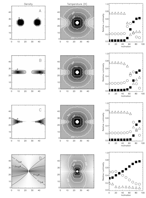
Figure 3: Density and temperature maps obtained for disk structure as well as its respective relative luminosity correlation plot.

For the 4 disk shapes adopted we obtained the temperature maps shown in Figure 3, column 2. These maps show the shadowing effect of the dense structures. With the calculated SEDs we also constructed plots with the correlations of the relative luminosities for each of the structures as a function of inclination angle, also shown in Figure 3, right most column. These can then be compared to the plots of Figure 1 which shows the observed behavior.

It is not trivial to compare the model result with the much “noisier” observational plot. The noise, or spread is likely caused by stellar and dust properties varying from object to object and also by the errors on estimating the inclination angles for each individual nebula. To make the comparison easier, we generated sets of model data by allowing the stellar and dust properties to vary randomly within a physically meaningful range of values. This simulates observing a large sample of “real” objects with difference parameters as was done in the observed sample, allowing a direct comparison of the model and observational samples.

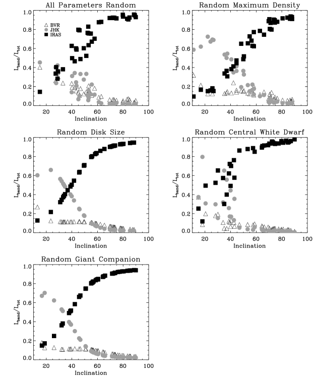
Figure 4: Model generated data sets for comparison with observed data. The parameters are allowed to vary randomly over a range defined in the text. The five graphs show: all parameters varying, only the disk size varying, the maximum density, the giant companion, and the white dwarf, all as indicated in the figure.

To accomplish this we ran a set of 29 models, equivalent to the observational sample we had, plotted in Figure 4. For each object the code was executed with input parameters selected in a random fashion with boundaries as described below:

Disk density: 5.0.10⁸ cm^-3; radius: 4.0.10¹⁵ cm
White Dwarf: T_Eff = 10⁵ K; Luminosity = 500 L_⊙
Giant: T_Eff = 5.10³ K; Luminosity = 1000 L_⊙

The parameters were allowed to vary in the range 0.5 to 1.0 times the parameter value in a uniform random distribution. The average physical characteristics of these disks are (in M_⊙:

Mass of dust in Disk = 3.64-05
Mass of Gas in Disk = 0.0044
Mass of Disk+Shell = 0.0048

The adopted shell has a radius of 10¹⁷ cm, a density of 1000 cm^-3, and simulates the presence of a generic planetary nebula in addition to the disk.

4 Absolute luminosity effects

Another predicted effect is that high inclination objects should have lower apparent luminosities because only the equatorial “donut” is seen, while for low inclination objects the central object and donut are observed, giving an apparent over-luminosity. Clearly, this effect is only possible in objects with an asymmetrical matter distribution. Averaging over all angles the total luminosity for a sample of objects is

L_tot = n.L_ave

so that energy is conserved. The excess luminosity of the low-i objects is exactly compensated by the under-luminous high-i objects.

To check the predicted behavior we generated a sample in the same way as done for the relative luminosity effect discussed above and plotted the observed luminosity as a function of inclination angle. The plot is shown in Figure 5.

Figure 5: Plot of the luminosities of a sample of BPNe as a function of inclination angle.

For a subset of seven objects we have reliable distances and therefore were able to determine their absolute luminosities. These objects are listed in Table 3 together with their luminosities, distances, and inclination angles.

Table 3: Objects for which distances are known with their observed luminosities. Listed are: Object, luminosity, distance, inclination angle. The average luminosities are for objects with i $\geq$ 45^o L = 346 L_⊙ and for i $\leq$ 45^o L = 3550 L_⊙.

Object	L(L⊙	d(pc)	i(o)
Sa 2-237	340	2100	70
M 2-9	553	640	75
He 2-104	205	800	50
He 2-111	440	2800	70
M 1-16	194	1800	70
R Aqr	2800	200	20
BI Cru	4300	180	40

There is a significant difference in the mean luminosities of the two groups, whereby the high-i group has the lower luminosity, as predicted. The standard deviation of the high-i group mean is 154 and of the low-i group 1060. The difference between the mean values is 3204 nearly a 3 $\sigma$ result.

Another sanity check on the randomness of the angle distribution on the sky is to count the number of objects in inclination angle bins and compare these with the theoretically expected numbers which should go as sin(i) if the distribution on the sky is truly random. We have 7% of objects in the 0-30^o bin, 52% in the 31-60^o bin, and 41% in the 61-90^o bin. Noting that there are 5 objects with 60^o inclinations which happen to fall in the 31-60^o bin. Distributing these equally over this and the next bin, we obtain 7%, 43%, and 50%. Theory predicts –by integrating sin(i) over the same three angle bins, respectively, 13%, 37%, and 50% of the objects in the bins, relatively close to the observed values, with or without the 60^o object correction.

5 Projected expansion velocities

The expansion velocities of BPNe with low inclinations should -all other things being equal- be on average higher than those of high inclinations objects. To test this idea for our sample we used the published expansion velocities from Corradi & Schwarz (1995). To correct as much as we can for intrinsic differences in expansion velocities between objects, we took the aspect ratio of an object to be proportional to its expansion velocity. This makes sense because the polar expansion compared to the typical PNe expansion of 15 km.s^-1 determines the aspect ratio of the object. Plotting the expansion velocity divided by aspect ratio against the inclination angle for all those objects for which we have data, we see in Figure 6 that there is a correlation between these parameters. When plotting the expansion velocity without correcting for the aspect ratio, the correlation is also there. This is unlikely to be physical and must be related to the projection of the true expansion velocities. In Table 4 we list the objects with their expansion velocities and aspect ratios.

Figure 6: Plot of the expansion velocities of our sample as a function of inclination angle corrected for the objects aspect ratio.

Table 4: Objects for which the expansion velocity is known with their aspect ratio.

Object	$V_{exp}$ ($km/s$)	Aspect Ratio (AR)
19W32	9	5.0
Hb5	106	2.2
He2-36	70	1.9
He2-111	127	4.0
IC4406	25	3.3
M1-16	127	5.3
M1-91	4	5.0
M2-9	69	12.0
MyCn18	14	2.0
Mz3	76	3.8
NGC2346	35	2.5
NGC2440	32	2.0
NGC2899	13	1.9
NGC6302	55	3.5
NGC6445	42	1.5
NGC6537	150	4.0
NGC7026	37	1.8
He2-104	125	10.0
BI Cru	214	10.0

6 Conclusions

The first and most obvious result is that a sharply changing density distribution cannot reproduce the observed behavior of the luminosity with inclination angle. The only models that agree well with the observations have the smoothly varying structure of the last row of Figure 3. We will continue calling this distribution a “disk”.

The 2-D model copes well with double central stars. By using a hot, compact star with a cooler giant-like companion, we get good agreement with the observations. Since we only have a relatively small sample of random systems the spread in our plots is rather large and a precise and detailed model cannot be selected on this basis. We do, however, confirm that the observed behavior as a function of inclination angle is easily reproducible with simple and physically meaningful and plausible models of bipolar nebulae.

References

- Corradi et al. (1998) Corradi, R.L.M., Aznar, R., Mampaso, A. 1998, MNRAS, 297, 617
- Corradi & Schwarz (1995) Corradi, R.L.M., Schwarz, H.E. 1995, A&A, 293, 871
- Gurzadyan (1997) Gurzadyan, G.A., 1997 “The Physics and Dynamics of Planetary Nebulae”, Springer Verlag
- Harpaz, Soker (1995) Harpaz, A., Soker, N. Eds. 1995, “Asymmetrical Planetary Nebulae”, Annals of the Israel Physical Soc., 11
- Kastner, Soker, Rappaport (2000) Kastner, J.H., Soker, N., Rappaport, S.A. Eds. 2000, “Asymmetrical Planetary Nebulae II”, ASP Conf. Proc. 199
- Li & Draine (2001) Li, A. & Draine, B. T. 2001, ApJ, 554, 778
- Melnick & Harwit (1975) Melnick, G., Harwit, M. 1975, MNRAS, 171, 441
- Meixner, Kastner, Balick, Soker (2004) Meixner, M., Kastner, J.H., Balick, B., Soker, N. Eds. 2004, “Asymmetrical Planetary Nebulae III”, ASP Conf. Proc., 313
- Phillips (1997) Phillips, J.P., 1997, A&A, 325, 755
- Soker (2004) Soker, N., 2004, in: Asymmetrical Planetary Nebulae III, ASP Conf. Proc., 313, 562 Eds. Meixner, M. et al
- Su, Hrivnak, Kwok (2001) Su, K.Y.L., Hrivnak, B.J., Kwok, S., 2001, AJ, 122, 1525