Cosmological neutrino mass limit and the dynamics of dark energy
Abstract
We investigate the correlation between the neutrino mass limit and dark energy with time evolving equation of state. Parameterizing dark energy as , we make a global fit using Markov Chain Monte Carlo technique to determine , neutrino mass as well as other cosmological parameters simultaneously. We pay particular attention to the correlation between neutrino mass and using current cosmological observations as well as the future simulated datasets such as PLANCK, SNAP and LAMOST.
pacs:
98.80.EsI Introduction
With the accumulation of high quality observational data of cosmic microwave background (CMB) Spergel:2006hy ; wmap3:2006 , large scale structure (LSS) of galaxies Cole:2005sx ; Tegmark:2003uf ; Tegmark:2003ud and Supernovae Type Ia (SN Ia) Tonry03 ; Riess04 ; Riess05 , we have been pacing into a new era of precision cosmology. In 1998, the analysis of the luminosity-redshift relation of SN Ia revealed the current acceleration of our universe Riess98 ; Perl99 . This acceleration attributes to a new form of energy, dubbed dark energy (DE), with negative pressure and almost not clustering whose nature remains unveiled. The simplest candidate of dark energy is the cosmological constant (CC) however it suffers from the fine tunning and coincidence problems SW89 ; ZWS99 . To ameliorate these dilemmas some dynamical dark energy models such as quintessence quint , phantom phantom , k-essence kessence and quintom whose equation of state (EOS) can cross -1 during evolution quintom have been proposed and studied thoroughly both theoretically and phenomenologically in the literature quintom ; Feng:2004ff ; xia ; Zhao:2005vj ; Xia:2005ge ; Xia:2006cr ; Zhao:2006bt ; Xia:2006rr ; Li:2005fm ; Zhang:2005eg ; Zhang:2006ck ; Guo:2004fq ; Copeland:2006wr ; relevnt .
Neutrino physics, especially the mass limit, is another challenge of modern science. The combined analysis of all currently available data of neutrino oscillation experiments implies the crucial mass differences in the neutrino mass hierarchy, say, eV2, eV2 for solar neutrino and the atmospheric neutrino mass difference respectively Aliani:2003ns . In the scenario of hierarchical neutrino masses these results suggest , , and . For the inverted hierarchy , , and . However, if the neutrino masses are degenerate, one finds . These oscillation experiments can merely constrain the squared mass differences, , they cannot detect the absolute value of neutrino masses which is of great significance.
However, cosmological observations can put upper limits of the absolute neutrino mass. For background evolution, neutrino masses contribute to the cosmic energy budget so that modify the epoch of matter-radiation equality, angular diameter distance to the last scattering surface (LSS) and other related physical quantities. For the perturbation, neutrinos become non-relativistic at late time thus they damp the perturbation within their free streaming scale. This suppressed the matter power spectrum by roughly Hu:1997mj . Dark energy can also affect the evolution of background and perturbation, which can mimic the behavior of neutrino to some extent, so that there exists an obvious correlation between equation of state of dark energy and neutrino mass.
For simplicity, Ref.Hannestad:2005gj ; Goobar:2006xz parameterizes dark energy by constant equation of state and finds it strongly correlates with neutrino mass. In this paper, we study this correlation with dynamical dark energy models which are more generic with current cosmological observations as well as with future simulated data. Further we have determined the parameters of dynamical dark energy and neutrino mass limit simultaneously.
The rest part of this paper is structured as follows: in the next section we present our fitting method and data we use. In section III we give our results. We make conclusion and discussion in the last section.
II Method and data
We choose the commonly used parametrization of the EOS of dark energy as Linder:2002et :
| (1) |
where is the redshift. Clearly the cosmological constant corresponds to thus CDM model is incorporated in this parametrization. For neutrino mass, we use the parameter which is defined as dark matter neutrino fraction:
| (2) |
where and denote the energy density of neutrino and dark matter respectively, is the sum of neutrino mass and is the physical cold dark matter densities relative to critical density.
The fitting and statistics strategy we adopt is based on the Markov Chain Monte Carlo package CosmoMC Lewis:2002ah 111Available at http://cosmologist.info/cosmomc/, which has been modified to implement dark energy perturbations with EOS getting across Zhao:2005vj . Our most general parameter space is
| (3) |
where and are the physical baryon and cold dark matter densities relative to critical density, is the ratio (multiplied by 100) of the sound horizon to the angular diameter distance at decoupling, is the optical depth, is defined as the amplitude of initial power spectrum and measures the spectral index. Assuming a flat Universe motivated by inflation and basing on the Bayesian analysis, we vary the 9 parameters above and fit to the observational data with the MCMC method. We take the weak priors as: 222We set the prior of and broad enough to ensure the EoS can evolve in the whole parameter space. and a cosmic age tophat prior as 10 Gyr20 Gyr. Furthermore, we make use of the HST measurement of the Hubble parameter freedman by multiplying the likelihood by a Gaussian likelihood function centered around and with a standard deviation . We impose a weak Gaussian prior on the baryon density (1) from Big Bang nucleosynthesis bbn .
In our global fitting we compute the total likelihood to be the products of separate likelihoods of CMB, SNIa, LSS and Heidelberg-Moscow experiment (HM) Kl04 ; Kl06 ; fogli2 . Alternatively defining , so
| (4) |
For CMB data we use the three-year WMAP (WMAP3) Temperature-Temperature (TT) and Temperature-Polarization (TE) power spectrum with the routine for computing the likelihood supplied by the WMAP team WMAP3IE . The supernova data we use are the “gold” set of 157 SNIa published by Riess in Riess04 . We have marginalized over the nuisance parameter DiPietro:2002cz in the calculation of SN Ia likelihood. For LSS information, we have used the 3-D matter power spectrum of SDSS Tegmark:2003uf and 2dFGRS Cole:2005sx , Lyman- forest data (Ly) from SDSS lya and recent measurement of the baryon acoustic oscillation feature in the 2-point correlation function of SDSS Eisenstein2005 . To be conservative but more robust, we only use the first 14 bins of the SDSS 3-D matter power spectrum, which are well within the linear regime sdssfit . For Ly likelihood, we modify the interpolating code333Available at http://www.cita.utoronto.ca/ pmcdonal/LyaF/public.lyafchisq.tar.gz to incorporate dynamical dark energy models. For BAO likelihood, we use the constraint444In this work we mainly focus on the correlation between dark energy parameters and the neutrino mass rather than the absolute value of the neutrino mass. What we are interested in is the possible effect of BAO measurement on this correlation. Since the BAO measurement seems not very consistent with the other observations, such as CMB and SN Ia, on the constraints of dark energy parameters, we don’t use the full power spectrum analysis of BAO in our calculations for simplicity. Similarly the author of Ref.Cirelli:2006kt also use the parameter A to study the neutrino mass limit. Eisenstein2005 :
| (5) |
| (6) |
where is the Hubble parameter, is the speed of light and is the comoving angular diameter distance at a specific redshift . Thus
| (7) |
Moreover, the Heidelberg-Moscow experiment uses the half time of decay to constrain the effective Majorana mass and this translates to the constraints of sum of neutrino mass under some assumptions DeLaMacorra:2006tu :
| (8) |
Given the Heidelberg-Moscow experiment is controversial for the time being and seems not consistent with other observational data, we just make a tentative fit choosing the HM prior to illustrate the effect on the correlation between the dark energy parameters and the neutrino mass when the total neutrino mass is very large.
To get robust conclusion, we have also used the simulated data from future observations of PLANCK, LAMOST and SNAP. The fiducial model we choose is the best-fit from the WMAP3 dataset Spergel:2006hy : , , , , and . And we assume the sum of neutrino mass and the equation of state of dark energy , .
For the CMB simulation we consider a simple full-sky () simulation at Planck-like sensitivity and ignore the lensing effect and the tensor information. We neglect foregrounds and assume the isotropic noise with variance (Pessimistic Planck-like sensitivity) and a symmetric Gaussian beam of 7 arcminutes full-width half-maximum (FWHM) Lewis:2005tp . We use the simulated up to for temperature and for polarization. The effective is:
| (9) |
where denote theoretical power spectra and denote the power spectra from the simulated data. The likelihood has been normalized with respect to the maximum likelihood, where Easther:2004vq ; Perotto:2006rj .
For the future LSS survey we consider LAMOST project. The Large Sky Area Multi-Object Fiber Spectroscopic Telescope (LAMOST) project as one of the National Major Scientific Projects undertaken by the Chinese Academy of Science, aims to measure galaxies with mean redshift lamost . In the measurements of large scale matter power spectrum of galaxies there are generally two statistical errors: sample variance and shot noise. The uncertainty due to statistical effects, averaged over a radial bin in Fourier space, is 9304022
| (10) |
The initial factor of 2 is due to the real property of the density field, is the survey volume and is the mean galaxy density. In our simulations for simplicity and to be conservative, we use only the linear matter power spectrum up to Mpc-1.
The projected satellite SNAP555SNAP is one of the several candidates emission concepts for the Joint Dark Energy Mission(JDEM). (Supernova / Acceleration Probe)would be a space based telescope with a one square degree field of view with 1 billion pixels. It aims to increase the discovery rate for SNIa to about 2,000 per year snap . The simulated SN Ia data distribution is taken from Refs.kim ; Li:2005zd . As for the error, we follow Ref.kim which takes the magnitude dispersion and the systematic error , and the whole error for each data is
| (11) |
where is the number of supernova in the ’th redshift bin.
For each regular calculation, we run 6 independent chains comprising of 150,000-300,000 chain elements and spend thousands of CPU hours to calculate on a cluster. The average acceptance rate is about 40%. And for the convergence test typically we get the chains satisfy the Gelman and Rubin GR92 criteria where R-10.1.
Despite our ignorance of the nature of dark energy, it is more natural to consider the DE fluctuation whether DE is regarded as scalar field or fluid rather than simply switching it off. The conservation law of energy reads:
| (12) |
where is the energy-momentum tensor of dark energy and “;” denotes the covariant differentiation. Working in the conformal Newtonian gauge, Equation(12) leads to the perturbation equations of dark energy as follows ma :
| (13) | |||||
| (14) |
For the models where the EOS doesn’t cross -1, the above equation(13), (14) is well defined. For the crossing models, the perturbation equation (13), (14) is seemingly divergent. However basing on the realistic two-field-quintom model as well as the single field case with a high derivative term Zhao:2005vj , the perturbation of DE is shown to be continuous when the EOS gets across -1, thus we introduce a small positive parameter to divide the full range of the allowed value of the EOS into three parts: 1) ; 2) ; and 3) .
For the regions 1) and 3) the perturbation is well defined by solving Eqs.(13), (14) as shown above. For the case 2), the perturbation of energy density and divergence of velocity, , and the time derivatives of and are finite and continuous for the realistic quintom dark energy models. However for the perturbations with the above parameterizations clearly there exists some divergence. To eliminate the divergence typically one needs to base on the multi-component DE models which result in the non-practical parameter-doubling. A simple way out is to match the perturbation in region 2) to the regions 1) and 3) at the boundary and set Zhao:2005vj ; Xia:2005ge ; Xia:2006cr
| (15) |
We have numerically checked the error in the range and found it less than 0.001 to the exact multi-field quintom model. Therefore our matching strategy is a perfect approximation to calculate the perturbation consistently for crossing models. For more details of this method we refer the readers to our previous companion papers Zhao:2005vj ; Xia:2005ge ; Xia:2006cr .
III Results
TABLE 1. Median values and 1 constrains on dark energy parameters and sum of neutrino mass for models discussed in the text. From left to right, we use WMAP three year data (WMAP3), WMAP3+Riess 157 “Gold” sample+2dF+SDSS(14bands)(LSS), WMAP3+LSS+Lyman- forest(Ly), WMAP3+LSS+Lyman-+Baryon Acoustic Oscillation (BAO) information, WMAP3+LSS+Ly+BAO+Heidelberg-Moscow experiment data respectively. The right most column we use the simulated data for future SNAP+PLANCK+LAMOST. For one-tailed distributed parameter such as neutrino mass, we quote the 95 C.L. limit.
| +Dynamical Dark Energy with Dark Energy Perturbation | ||||||
| WMAP3 | +SN+LSS | +Ly | +BAO | +Heidelberg-Moscow | Planck+SNAP+LAMOST | |
| 0.110 | 0.086 | 0.0005 | ||||
| +Dynamical Dark Energy without Dark Energy Perturbation | ||||||
| WMAP3 | +SN+LSS | +Ly | +BAO | +Heidelberg-Moscow | Planck+SNAP+LAMOST | |
| 0.041 | 0.013 | 0.089 | ||||
| +WCDM with Dark Energy Perturbation | ||||||
| WMAP3 | +SN+LSS | +Ly | +BAO | +Heidelberg-Moscow | Planck+SNAP+LAMOST | |
| +CDM | ||||||
| WMAP3 | +SN+LSS | +Ly | +BAO | +Heidelberg-Moscow | Planck+SNAP+LAMOST | |
In this section we present our global fitting results of dark energy parameters and neutrino mass limit. We pay particular attention to the correlation between , which delineates the time evolving of dark energy, and neutrino mass. Our main result was summarized in Table I. We choose the general model of 9 free parameters as illustrated in Eq.(3) to study the correlation between dynamical dark energy and neutrino mass and discuss the model with DE with constant equation of state (WCDM) and CDM model for comparison. Here we only list the parameters of dark energy and neutrino mass. Since dark energy perturbation is crucial in determination of cosmological parameters especially for dark energy parameters Spergel:2006hy ; Zhao:2005vj ; Xia:2005ge ; Zhao:2006bt , we include the full dark energy perturbation in our global fitting as well as showing the result by incorrectly switching off dark energy perturbations to reinforce this key point. We use different data combination discussed in previous section. The cov(X,Y) is the correlation coefficient of samples which quantifies the correlation between the two parameters X and Y defined ascorr :
| (16) |
where the bar denotes the mean value of parameters. If cov(X,Y)0 means X,Y is positively correlated and vice versa.
From the comparison of results with/without dark energy perturbation, we find dark energy perturbation modifies the mean value of all the parameters as well as enlarging the corresponding errors which is consistence with previous analysis in the literature Spergel:2006hy ; Zhao:2005vj ; Xia:2005ge ; Zhao:2006bt . We will merely discuss the results with dark energy perturbation hereafter. We have seen that WMAP3 only put weak constraints on and neutrino mass since CMB data is sensitive to the effective equation of state of dark energy defined as Wang:1999fa :
| (17) |
thus it’s hard to constrain and neutrino mass by CMB data alone. Adding SN Ia and LSS data we find the mean value of each parameter gets modified and the error bars shrink a lot. However it is noteworthy that adding BAO data enlarges the error of while tightens the neutrino mass limit to a great extent. If we take the HM prior in Eq.(8), we find the error of become greater while the 1-D posterior distribution of neutrino mass turns to be two-tailed. We have also done the global fitting using the simulated data of future observation and found the errors shrink greatly.
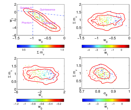
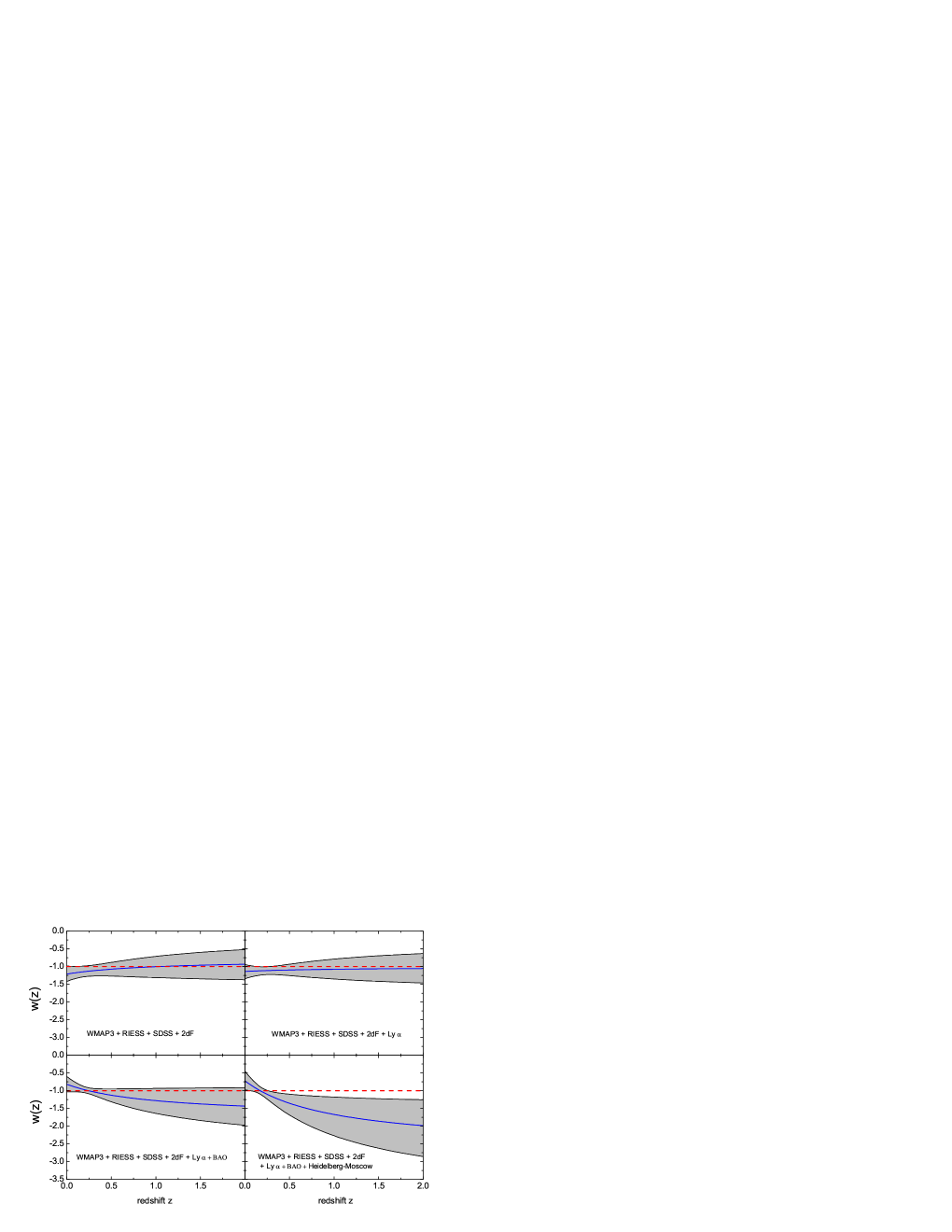
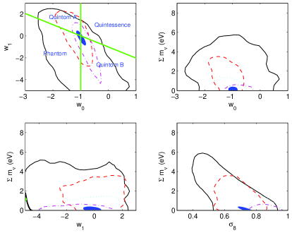
In Fig.(1) we show the C.L. 2-D contours of , neutrino mass and . From outside in, we add data as illustrated in the figure caption. Using simulated data we obtain the inner most shaded regions. The contours shrink significantly while interesting correlations remain. The results including HM prior are illustrated in Fig.(2). We also cut the plane into four parts for different dark energy models as we did in Xia:2005ge ; Xia:2006cr ; Zhao:2006bt . The EOS of Quintom A crossing -1 from upside down, i.e. the EOS is greater than -1 in the early epoch yet negative than -1 currently while quintom B crosses -1 from the opposite direction. We find that the CDM model cannot be ruled out by all the data combination at level however the quintom-like dynamical dark energy model is mildly favored. The one dimensional constraints of EOS by different combination of datasets are illustrated in Fig.(3). We find that the best fit models are always allowed crossing the boundary in these four combinations. When adding the dataset of BAO measurement or HM measurement the direction of EOS crossing the boundary will be changed. This is due to the changed sign of the mean value of . And the HM prior seems favor more negative value of and stronger evolution of EOS.
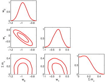
In Ref.Hannestad:2005gj , the author just used the constant EOS to consider the correlation between EOS of dark energy and neutrino mass. The critical point of our result is the correlation among and neutrino mass. From the table I we find there exists some correlation of () and especially for and . More interestingly, we find using future high quality data, the correlation between and nearly vanishes while there is a strong and negative correlation between the “running” of dark energy EOS and the total neutrino mass . Fig.(4) delineates the fitting result of future simulation in more detail and we clearly see the strong correlations between and neutrino mass. In Ref.Ichikawa:2005hi , the authors conclude is not strongly correlated with neutrino mass basing on Fisher matrix analysis. However, we have seen the distribution of and neutrino mass is highly non-Gaussian and Fisher matrix technique is not viable in such cases Perotto:2006rj . Furthermore, they didn’t consider dark energy perturbation when EOS crosses . This also give rise to great bias of determining neutrino mass limit if neglecting time evolving of dark energy as illustrated in the table I.
The reason of the correlation between and dark energy is not hard to understand. The main correlation between dark energy EOS and neutrino mass stems from the geometric feature of our universeHannestad:2005gj . In addition, dynamical dark energy will modify the time evolving potential wells which affects CMB power spectra through the late time ISW effect. Dynamical dark energy can leave imprints on CMB, LSS power spectrum and Hubble diagram nonetheless these features can be mimicked by cosmic neutrino to some extentCorasaniti:2002bw . This is the source of correlation.
IV Conclusion
In this paper we have done the global fitting including parameters expressing time evolving dark energy, neutrino mass and other 6 cosmological parameters using different combination of currently data as well as simulated data for future observation. We have seen the interesting correlation between neutrino mass and EOS of time evolving dark energy especially for and . The correlation between the “running” of dark energy EOS and the total neutrino mass is of great significance in determining neutrino mass limit and revealing the nature of dark energy by futuristic high precision observational data, such as SNAP, PLANCK666http://sci.esa.int/planck/ and so forth.
Acknowledgements: We acknowledge the use of the Legacy Archive for Microwave Background Data Analysis (LAMBDA). Support for LAMBDA is provided by the NASA Office of Space Science. Our MCMC chains were finished in the Shuguang 4000A system of the Shanghai Supercomputer Center(SSC). This work is supported in part by National Natural Science Foundation of China under Grant Nos. 90303004, 10533010 and 19925523. We are indebted to Patrick Mcdonald and Anze Slosar for clarifying correspondence on the fittings to the Lyman data. We thank Antony Lewis for technical support on cosmocoffee777http://cosmocoffee.info. We thank Bo Feng, Hiranya Peiris, Mingzhe Li, Pei-Hong Gu, Hong Li and Xiao-Jun Bi for helpful discussions and comments on the manuscript.
References
- (1)
- (2) D. N. Spergel et al., arXiv:astro-ph/0603449.
- (3) L. Page et al., arXiv:astro-ph/0603450. G. Hinshaw et al., arXiv:astro-ph/0603451. N. Jarosik et al., arXiv:astro-ph/0603452.
- (4) S. Cole et al. [The 2dFGRS Collaboration], Mon. Not. Roy. Astron. Soc. 362 (2005) 505
- (5) M. Tegmark et al. [SDSS Collaboration], Astrophys. J. 606, 702 (2004)
- (6) M. Tegmark et al. [SDSS Collaboration], Phys. Rev. D 69, 103501 (2004)
- (7) J. L. Tonry et al. (Supernova Search Team Collaboration), Astrophys. J. 594, 1 (2003).
- (8) A. G. Riess et al. (Supernova Search Team Collaboration), Astrophys. J. 607, 665 (2004).
- (9) A. Clocchiatti et al. (the High Z SN Search Collaboration), Astrophys. J. 642, 1 (2006).
- (10) A.G. Riess et al. (Supernova Search Team Collaboration), Astron. J. 116, 1009 (1998).
- (11) S. Perlmutter et al. (Supernova Cosmology Project Collaboration), Astrophys. J. 517, 565 (1999).
- (12) S. Weinberg, Rev. Mod. Phys. 61, 1 (1989).
- (13) I. Zlatev, L.-M. Wang, and P. J. Steinhardt, Phys. Rev. Lett. 82, 896 (1999).
- (14) R. D. Peccei, J. Sola and C. Wetterich, Phys. Lett. B 195, 183 (1987); C. Wetterich, Nucl. Phys. B 302, 668 (1988); B. Ratra and P. J. E. Peebles, Phys. Rev. D 37, 3406 (1988). P. J. E. Peebles and B. Ratra, Astrophys. J. 325, L17 (1988).
- (15) R. R. Caldwell, Phys. Lett. B 545, 23 (2002)
- (16) T. Chiba, T. Okabe and M. Yamaguchi, Phys. Rev. D 62 (2000) 023511 C. Armendariz-Picon, V. F. Mukhanov and P. J. Steinhardt, Phys. Rev. Lett. 85, 4438 (2000)
- (17) B. Feng, X. L. Wang and X. M. Zhang, Phys. Lett. B 607, 35 (2005)
- (18) B. Feng, M. Li, Y. S. Piao and X. Zhang, Phys. Lett. B 634, 101 (2006)
- (19) J.-Q. Xia, B. Feng, and X. Zhang, Mod. Phys. Lett. A 20, 2409 (2005).
- (20) G. B. Zhao, J. Q. Xia, M. Li, B. Feng and X. Zhang, Phys. Rev. D 72, 123515 (2005).
- (21) J. Q. Xia, G. B. Zhao, B. Feng, H. Li and X. Zhang, Phys. Rev. D 73, 063521 (2006)
- (22) J. Q. Xia, G. B. Zhao, B. Feng and X. Zhang, JCAP 0609, 015 (2006).
- (23) G. B. Zhao, J. Q. Xia, B. Feng and X. Zhang, arXiv:astro-ph/0603621.
- (24) J. Q. Xia, G. B. Zhao, H. Li, B. Feng and X. Zhang, Phys. Rev. D 74, 083521 (2006).
- (25) M. Li, B. Feng and X. Zhang, JCAP 0512, 002 (2005)
- (26) X. F. Zhang, H. Li, Y. S. Piao and X. M. Zhang, Mod. Phys. Lett. A 21, 231 (2006)
- (27) X. F. Zhang and T. Qiu, Phys. Lett. B 642, 187 (2006).
- (28) Z. K. Guo, Y. S. Piao, X. M. Zhang and Y. Z. Zhang, Phys. Lett. B 608, 177 (2005)
- (29) For a review see E. J. Copeland, M. Sami and S. Tsujikawa, Int. J. Mod. Phys. D 15, 1753 (2006).
- (30) e.g. H. Wei and R.-G. Cai, Class. Quant. Grav. 22, 3189 (2005); R.-G. Cai, H.-S. Zhang and A. Wang, Commun. Theor. Phys. 44, 948 (2005); A. A. Andrianov, F. Cannata and A. Y. Kamenshchik, Phys. Rev. D 72, 043531 (2005); X. Zhang, Int. J. Mod. Phys. D 14, 1597 (2005); Q. Guo and R.-G. Cai, arXiv:gr-qc/0504033; B. McInnes, Nucl. Phys. B 718, 55 (2005); I. Y. Aref’eva, A. S. Koshelev, and S. Yu. Vernov, Phys. Rev. D 72, 064017 (2005); C. G. Huang and H. Y. Guo, arXiv:astro-ph/0508171; W. Zhao and Y. Zhang, Phys. Rev. D 73, 123509 (2006); J. Grande, J. Sola and H. Stefancic, JCAP 0608, 011 (2006); L. P. Chimento and R. Lazkoz, Phys. Lett. B 639, 591 (2006); F. Cannata and A. Y. Kamenshchik, arXiv:gr-qc/0603129; R. Lazkoz and G. Leon, Phys. Lett. B 638, 303 (2006); B. Feng, arXiv:astro-ph/0602156; H. Stefancic, J. Phys. A 39, 6761 (2006) ; L. Perivolaropoulos, AIP Conf. Proc. 848, 698 (2006).
- (31) P. Aliani, V. Antonelli, M. Picariello and E. Torrente-Lujan, hep-ph/0309156; P. C. de Holanda and A. Y. Smirnov, Astropart. Phys. 21, 287 (2004); M. Maltoni, T. Schwetz, M. A. Tortola and J. W. F. Valle, Phys. Rev. D 68, 113010 (2003).
- (32) W. Hu, D. J. Eisenstein and M. Tegmark, Phys. Rev. Lett. 80, 5255 (1998).
- (33) S. Hannestad, Phys. Rev. Lett. 95, 221301 (2005).
- (34) A. Goobar, S. Hannestad, E. Mortsell and H. Tu, JCAP 0606, 019 (2006).
- (35) E. V. Linder, Phys. Rev. Lett. 90, 091301 (2003).
- (36) A. Lewis and S. Bridle, Phys. Rev. D 66, 103511 (2002).
- (37) W. L. Freedman et al., Astrophys. J. 553, 47 (2001).
- (38) S. Burles, K. M. Nollett and M. S. Turner, Astrophys. J. 552, L1 (2001).
- (39) H.V. Klapdor-Kleingrothaus, I.V. Krivosheina, A. Dietz, and O. Chkvorets, Phys. Lett. B 586, 198 (2004).
- (40) H.V. Klapdor-Kleingrothaus, talk at SNOW 2006, 2nd Scandinavian Neutrino Workshop (Stockholm, Sweden, 2006).
- (41) G. L. Fogli et al., hep-ph/0608060.
- (42) Available from http://lambda.gsfc.nasa.gov/product/map/current/.
- (43) For details see e.g. E. Di Pietro and J. F. Claeskens, Mon. Not. Roy. Astron. Soc. 341, 1299 (2003).
- (44) P. McDonald et al. [SDSS Collaboration], Astrophys. J. 635, 761 (2005).
- (45) D. J. Eisenstein et al. [SDSS Collaboration], Astrophys. J. 633, 560 (2005).
- (46) M. Tegmark et al. [SDSS Collaboration], Phys. Rev. D 69, 103501 (2004).
- (47) M. Cirelli and A. Strumia, JCAP 0612, 013 (2006).
- (48) A. De La Macorra, A. Melchiorri, P. Serra and R. Bean, arXiv:astro-ph/0608351.
- (49) A. Lewis, Phys. Rev. D 71, 083008 (2005).
- (50) R. Easther, W. H. Kinney and H. Peiris, JCAP 0505, 009 (2005).
- (51) L. Perotto, J. Lesgourgues, S. Hannestad, H. Tu and Y. Y. Y. Wong, JCAP 0610, 013 (2006).
- (52) Available at http://www.lamost.org/.
- (53) H. A. Feldman, N. Kaiser and J. A. Peacock, Astrophys. J. 426, 23 (1994).
- (54) Available at http://snap.lbl.gov/.
- (55) A. G. Kim, E. V. Linder, R. Miquel and N. Mostek, Mon. Not. Roy. Astron. Soc. 347, 909 (2004).
- (56) H. Li, B. Feng, J. Q. Xia and X. Zhang, Phys. Rev. D 73, 103503 (2006).
- (57) A. Gelman and D. Rubin, Statistical Science 7, 457 (1992).
- (58) C. -P. Ma and E. Berschinger, Astrophys. J. 455, 7 (1995).
- (59) Bhattacharyya,G.K. and R.A.Johnson, Statistical Concepts and Methods. New York: John Wiley, 1977.
- (60) e.g. L. M. Wang, R. R. Caldwell, J. P. Ostriker and P. J. Steinhardt, Astrophys. J. 530, 17 (2000).
- (61) K. Ichikawa and T. Takahashi, arXiv:astro-ph/0510849.
- (62) P. S. Corasaniti, B. A. Bassett, C. Ungarelli and E. J. Copeland, Phys. Rev. Lett. 90, 091303 (2003).