Characterizing Three Candidate Magnetic CVs from SDSS: XMM-Newton and Optical Follow-up Observations^⋆

Abstract

In the latest in our series of papers on XMM-Newton and ground-based optical follow-up of new candidate magnetic cataclysmic variables (mCVs) found in the Sloan Digital Sky Survey, we report classifications of three systems: SDSS J144659.95+025330.3, SDSS J205017.84–053626.8, and SDSS J210131.26+105251.5. Both the X-ray and optical fluxes of SDSS J1446+02 are modulated on a period of $48.7\pm 0.5$ min, with the X-ray modulation showing the characteristic energy dependence of photo-electric absorption seen in many intermediate polars (IP). A longer period modulation and radial velocity variation is also seen at around 4 hrs, though neither dataset is long enough to constrain this longer, likely orbital, period well. SDSS J2050–05 appears to be an example of the most highly magnetized class of mCV, a disk-less, stream-fed polar. Its 1.57 hr orbital period is well-constrained via optical eclipse timings; in the X-ray it shows both eclipses and an underlying strong, smooth modulation. In this case, broadly phase-resolved spectral fits indicate that this change in flux is the result of a varying normalization of the dominant component (a 41 keV mekal), plus the addition of a partial covering absorber during the lower flux interval. SDSS J2101+10 is a more perplexing system to categorize: its X-ray and optical fluxes exhibit no large periodic modulations; there are only barely detectable changes in the velocity structure of its optical emission lines; the X-ray spectra require only absorption by the interstellar medium; and the temperatures of the mekal fits are low, with maximum temperature components of either 10 or 25 keV. We conclude that SDSS J2101+10 can not be an IP, nor likely a polar, but is rather most likely a disc accretor– a low inclination SW Sex star.

1. Introduction

The Sloan Digital Sky Survey (SDSS; York et al., 2000) has provided a wealth of new cataclysmic variables; the close binary systems with active accretion from a late main sequence star to a white dwarf (reviewed in Warner, 1995). Due to its sensitivity down to $\sim$21st mag, SDSS is especially suited to the discovery of faint CVs with low accretion rates and short orbital periods. Included in the discoveries are dozens of systems with a noticeable emission line of He II, which is often a signature of a white dwarf with a high magnetic field. The highest field systems (polars) have no accretion disk and the white dwarf spin is synchronized to the orbit. The intermediate polars (IPs) usually have some outer disk, with magnetic curtains channelling the inner disk material to the magnetic poles of the white dwarf which is spinning faster than the orbital timescale. Polars can be identified by circular polarization, cyclotron harmonics and/or Zeeman splitting (review in Wickramasinghe & Ferrario, 2000), while IPs are found through the detection of their spin and orbital periods. In addition, there is a class of high accretion rate disk systems with possible low magnetic field white dwarfs (Rodríguez-Gil et al., 2001), termed SW Sex stars, which can also show strong He II lines in their optical spectra.

For the last few years, we have used XMM-Newton to identify the nature of the CVs with He II and to explore the nature of X-ray heating in these systems. Polars generally exhibit hard X-rays from the accretion shock and soft X-rays from the white dwarf surface heated by the hard X-rays. The ratio of soft to hard X-rays shows a dramatic change with magnetic field strength and accretion rate. The IPs are generally hard X-ray emitters with large absorption effects from the accretion curtains. Usually the spin period is much more pronounced in the X-ray than the optical. The SW Sex stars usually show no X-ray variation and are hard X-ray emitters with low absorption.

The 3 sources in this study are all about 18th mag in the SDSS $g$ filter and were all identified as potential magnetic CVs in Szkody et al. (2003a). SDSS J144659.95+025330.3 (hereafter SDSS J1446+02) showed no polarization and limited time-resolved spectra could not determine the orbital period. SDSS J205017.85–053626.8 (SDSS J2050–05) has the strongest He II line of the 3 objects, with a peak flux comparable to H$\beta$ and showed evidence of high and low states of mass transfer. A short span of time-resolved spectroscopy showed an orbital period near 2 hrs. Followup high speed photometry by Woudt et al. (2004) revealed brief (260s), deep (1.5 mag) eclipses and determined a precise period of 1.57 hrs. The third system, SDSS J210131.26+105251.5 (SDSS J2101+10) has very strong Balmer lines but did not show any velocity variation during 1.3 hr of time-resolved spectroscopy.

The XMM-Newton data obtained on these 3 sources, combined with additional photometry, spectroscopy and spectropolarimetry has allowed us to determine that SDSS J1446+02 is an IP, SDSS J2050–05 is a likely polar, while SDSS J2101+10 escapes an easy classification, but appears most likely to be an SW Sex star. Our observations and results are described below.

2. Observations

Table 1Observation Summary

SDSS J	UT Date	Obs	UT Time	Characteristics	Comments
SDSS J1446+02	2002 May 11	SO: Bok (2.3m)	$\cdots$	$v=+0.38$%	3ks exposure, spectropolarimetry
	2003 Apr 27	APO	05:43 – 09:47	$\cdots$	$23\times 600$s spectra
	2003 May 07	NOFS	06:39 – 11:34	$\sim$$V=17.9$	open filter photometry
	2004 Jan 30	XMM-Newton:
		EPIC-pn	04:17 – 05:32	0.2 cts s-1	only 3.0ks live time
		EPIC-MOS1/2	03:55 – 05:18	0.1 cts s-1	only 4.5ks live time
		OM	04:03 – 08:10	$B=18.3$	13.9ks duration
		NOFS	09:13 – 13:18	$\sim$$V=18.2$	open filter photometry
	2005 Jan 12	XMM-Newton:
		EPIC-pn	06:22 – 08:09	0.20 cts s-1	5.6ks live time
		EPIC-MOS1/2	06:00 – 08:14	0.10 cts s-1	7.7ks live time
		OM	06:08 – 08:16	$B=18.2$	5.6ks duration
SDSS J2050–05	2003 May 29	MMT	$\cdots$	$v=+1.06$%	1.2ks exposure, spectropolarimetry
	2003 May 30	MMT	$\cdots$	$v=-0.23$%	2.4ks exposure, spectropolarimetry
	2004 May 14	SO: Bok (2.3m)	$\cdots$	$v=-0.31$%	1.2ks exposure, spectropolarimetry
	2004 Oct 18	XMM-Newton:
		EPIC-pn	10:13 – 13:17	0.67 cts s-1	8.7ks live time
		EPIC-MOS1/2	09:50 – 13:22	0.21 cts s-1	12ks live time
		OM	06:08 – 08:16	$B=18.4$	8.4ks duration
	2004 Oct 21	NOFS	01:33 – 04:34	$\sim$$V=18.0$	open filter photometry
SDSS J2101+10	2003 May 29	SO	$\cdots$	$v=+0.03$%	1.6ks exposure, spectropolarimetry
	2003 Sep 22	SO: Bok (2.3m)	$\cdots$	$v=+0.10$%	1.6ks exp., $R$-band imaging polarimetry
	2004 May 14	APO	10:47 – 11:04	$\cdots$	1ks spectrum
	2004 May 19	NOFS	08:01 – 11:35	$\sim$$V=18.9$	open filter photometry
	2004 May 19	XMM-Newton:
		EPIC-pn	16:57 – 18:13	0.64 cts s-1	4.1ks live time
		EPIC-MOS1/2	16:35 – 18:18	0.23 cts s-1	6.1ks live time
		OM	16:43 – 18:20	$B=19.0$	5.5ks duration

2.1. X-ray

Table 1 summarizes our X-ray and optical observations. SDSS J1446+02 was observed twice by XMM-Newton, as the 2004 January 30 observation was badly affected by high charged particle background throughout, and the X-ray exposures were curtailed after only a few kiloseconds. Since the X-ray instrumentation (comprising three X-ray telescopes, backed by the two MOS and one pn EPIC CCD cameras, Turner et al., 2001) was set as the prime instrument, an automatic reobservation was triggered. However, the 2004 optical data from XMM-Newton’s optical monitor (OM, Strüder et al., 2001) were good throughout the scheduled $\sim$13 ks observation. In the second observation on 2005 January 12, good data were obtained from all three EPIC spectro-imagers, but this time the OM only succeeded for 2 out of an expected 4 exposures. We note that for both observations no useful data were available from the two Reflection Grating Spectrographs (den Herder et al., 2001) arrayed in the optical path of the MOS detectors, as the source is too faint to furnish adequate signal in the dispersed spectra. The initial visits made to SDSS J2050–05 and SDSS J2101+10 were highly successful, with only a little background flaring in the last 3 ks of the 12 ks observation of SDSS J2050–05, and none affecting that of SDSS J2101+10. Useful data were therefore obtained from EPIC imaging and the OM, though once again neither target was bright enough for the RGS.

For the extraction of spectra and lightcurves from the XMM-Newton data we used the tools available in the Science Analysis System (SAS ) version 6.5.0, with calibration files current to 2005 December 15, and followed the standard protocol as given by the ESA XMM-Newton website and the ABC guide from the US GOF. In all cases we produced new event list files from the Observation Data Files to incorporate the latest calibration updates and then filtered them with the standard canned expressions. We defined circular source extraction regions (radii of 480 and 360 pixels for the MOS and pn camera respectively), centered on the centroid of the source, enclosing $\sim 80\%$ of the energy to optimize for signal-to-noise. Simple annular background extraction regions were defined on the same central MOS chip for those 2 cameras; for the pn we used adjacent rectangular regions at similar detector Y locations to the target. We also reprocessed the OM data with omfchain extracting lightcurves using more appropriate (for our relatively faint targets) source aperture and background regions to maximize signal-to-noise. We also chose binning to match that of the ground-based photometry, and lastly, to aid comparison, converted count rates to $B$ magnitudes.

The SAS task evselect performed the extractions of both X-ray spectra and lightcurves for source and background. For SDSS J1446+02 and SDSS J2050–05 further time filtering was applied to the event lists prior to spectral extraction to excise intervals of high X-ray background; the revised good time intervals (GTIs) were generated by setting limits on the count rate in hard ($>10$keV) lightcurves for the entire detector. We also restricted acceptable events to singles in the pn (pattern=0) but up to quadruples in the MOS (pattern$\leq 12$) to further improve energy resolution. In contrast, in extracting lightcurves only the standard GTIs were invoked, and we kept both singles and doubles for the pn (pattern$\leq 4$), to both maximize lightcurve coverage and signal-to-noise. For SDSS J2101+10 we also restricted the energy range to below 2.5 keV, where the source contributions dominate. SAS tasks rmfgen, arfgen and backscale generated appropriate redistribution matrix (rmf) and ancillary response files (arf) and calculated the relative scaling of source to background.

The final steps in data reduction utilized general purpose utilities in the FTOOLS software suite: grppha grouped the spectral bins and associated various files ready for spectral analysis in XSPEC; lcmath created background subtracted lightcurves, and combined the two MOS lightcurves, while earth2sun applied a correction to the time stamps for the solar system barycenter.

2.2. Optical

Ground based photometry was obtained for all three sources using the US Naval Observatory Flagstaff Station (NOFS) 1m telescope and a 2048 $\times$2048 CCD. An open filter was used which is close to a $V$ response and the magnitudes were calibrated from separate nights of all-sky photometry with Landolt standards. Light curves were made by using differential photometry with respect to comparison stars in each field and the magnitudes measured using IRAF routines. For SDSS J1446+02, 4 hrs of photometry began about one hour after the XMM-Newton observation ended on 2004 Jan 30. No data were obtained for the second observation but an additional 5 hrs of photometry from 2003 May 07 was used to establish the optical period. For SDSS J2050–05, 3 hrs of photometry were obtained 3 days after the XMM-Newton observations, while the 3.5 hrs of observations for SDSS J2101+10 took place 5.5 hrs prior to the start of XMM-Newton coverage. In all cases, the ground-based measurements agreed with the OM in showing the systems were all in their normal state of accretion.

In order to determine the orbital period for SDSS J1446+02, 4 hrs of time-resolved spectra were obtained on 2003 Apr 27. The Double Imaging Spectrograph (DIS) was used on the 3.5m telescope of the Apache Point Observatory (APO). Twenty three 10 min blue and red spectra were obtained with a 1.5″ slit, covering the regions 4200-5100Å and 6300-7200Å with a resolution of about 2Å. IRAF routines were used to calibrate the spectra for wavelength and flux using standards from the night. Velocities were measured for the prominent emission lines using the centroid (“e”) routine in the IRAF splot package; a double-Gaussian method (Shafter, 1983) was tried as well. A single spectrum of SDSS J2101+10 was also obtained at APO 5 nights before the XMM-Newton observation. The Balmer and He II strengths are very similar to the SDSS spectrum shown in Szkody et al. (2003a).

Circular spectropolarimetry was also performed for the three systems in a search for evidence of magnetic fields. The CCD spectropolarimeter SPOL was used (Schmidt et al., 1992) on the Steward Observatory 2.3 m Bok telescope and the 6.5 m MMT, as indicated in Table 1. All measurements on SDSS J1446+02 and SDSS J2101+10, and two of the three on SDSS J2050$-$05, yielded spectrum-averaged values $|v|=|V/I|<0.4\%$. Each result is well within $3\sigma$ of zero, and thus consistent with being unpolarized. However, a third epoch on SDSS J2050$-$05, obtained on 2003 May 29 in good observing conditions at the MMT, yielded $|v|=+1.06\%$. The S/N of these data is sufficient to reveal that the circular polarization rises continuously from $v\sim 0$ at $\sim$4200 Å to $v\sim 3\%$ beyond $\lambda=8000$ Å. This and other evidence for polarization by cyclotron emission in SDSS J2050$-$05 is discussed in $\S$4.2.

3. Analysis and results

3.1. X-ray Spectral Fitting

The extracted spectra were binned at $>$20 counts/bin, to facilitate the use of $\chi^{2}$ statistics to find the best model fits. For all sources the background contributed less than 3% of the flux within the source aperture, hence simpler fitting of background subtracted spectra was deemed acceptable. At the very lowest energies the calibration of the EPIC detectors remains uncertain; following the latest guidelines we restricted our fitting to $>0.2$keV for the MOS and $>0.15$keV for the pn. In every case, we performed joint fits to the data from all three X-ray cameras simultaneously, where all model parameters were fixed apart from the relative normalization of the pn relative to the MOS (which were assumed to be identical). In the cases where we separated the data into two phase or time bins, we then had 6 datasets. Starting from the case where all relative normalizations, as well as other model parameters, were kept constant, we then allowed normalizations to vary (but keeping the MOS to pn ratios constant), and then other model parameters like temperature, $F$-testing to see whether the additional degrees of freedom were statistically warranted each time. The best fits we present in figures and tables are those where the model has the fewest free parameters (i.e. leaves the most degrees of freedom); any further freeing of parameters did not then signficantly reduce the (reduced) $\chi^{2}$ values.

Furthermore, in finding the best fit models we always started from the simplest single emission component, solely absorbed by interstellar dust, with an initial value for $N_{H}$ as predicted by dust maps for the appropriate line of sight through the Galaxy. Typically, we used a single bremsstrahlung or a version including explicit line emission– the XSPEC model mekal– as expected for the optically thin thermally-emitting plasma encountered in CVs. In all cases, these simplest models failed to provide a good fit, hence we moved onto a variety of more complex combinations, e.g. multi-temperature or two-temperature thermal plasmas, additional soft blackbody components (as emitted by the heated polar caps in polars) and the effects of local partial covering absorption (i.e. due to obscuration by the accretion stream and/or curtain). We discuss the details of the best fits, as we report the results of our various analyses for each target in turn.

3.2. SDSS J1446+02

Table 2X-ray Spectral Fits for SDSS J1446+02

Model	reduced	$N_{H}$	Partial covering		Emission
	$\chi^{2}$	$\times 10^{20}$	$N_{H}$	frac.	model parameters
	(d.o.f.)	cm-2	($\times 10^{22}$cm-2)
bremss	1.5 (139)	$6.4\tablenotemark{a}$	$\cdots$	$\cdots$	$kT=200$ (pegged)
power law	1.11 (136)	$1.4^{+0.8}_{-1.0}$	$0.8\pm 0.2$	$0.41^{+0.04}_{-0.07}$	$\Gamma=1.2\pm 0.2$
multi-$T$ mekal	1.14 (137)	$1.6\pm 0.7$	$1.3\pm 0.2$	$0.64\pm 0.02$	$kT_{\rm max}=60$ keV (fixed)
					$\alpha=1.0$ (fixed)
2 $T$ mekal	1.10(134)	$4^{+27}_{-2}$	$0.9^{+3.9}_{-0.2}$	$0.47^{+0.05}_{-0.04}$	$kT_{1}=130^{+2}_{-4}\;$eV
					$kT_{2}=80^{+0}_{-19}$ keV
Joint fit to phase-selected “maximum” and “minimum” flux intervals:
2 $T$ mekal	1.08 (104)	$13^{+2}_{-3}$	none (max)	none (max)	$kT_{1}=81^{+4}_{-0}$ eV
			$4.4^{+1.6}_{-0.8}$(min)	$0.61\pm 0.03$(min)	$kT_{2}=58^{+22}_{-19}$ keV

Figure 1.— Radial velocities for the H$\alpha$ emission line in SDSS J1446+02, phase folded on the best fit period, $P=3.8\pm 0.3$ hrs. Overplotted is the sinusoid fit with $K=105\pm 11$ km s^-1 and $\gamma=-8\pm 5$ km s^-1.

3.2.1 Search for periodicities

From our APO spectroscopy run on SDSS J1446+02, we generated radial velocity curves for the prominent emission lines. A least square sine fit to the velocities was then used to determine the systemic velocity, the semi-amplitude, the orbital period and the phase (based on the red-to-blue crossing). While the H$\alpha$, H$\beta$, H$\gamma$ and He II lines were all measured, there were large deviations with respect to the best fit sine wave in all cases (total sigma of the fit of 34, 46, 75 and 73 km/s respectively), hence we only consider the fit to the H$\alpha$ curve in any detail (shown in fig. 1). All lines gave a period solution near 4 hrs, which is very close to the length of the dataset. The H$\alpha$ solution shown in figure 1 is for a period of $3.8\pm 0.3$ hrs, $K=105\pm 11$ km s^-1 and $\gamma$ of $-8\pm 5$ km s^-1, with red-to-blue crossing (phase 0) at 7:30 UT on 2003 Apr 27. Because the period is so close to the length of the observation, it is not a robust determination, but useful in showing that the orbital period is not short (i.e. under 2 hrs).

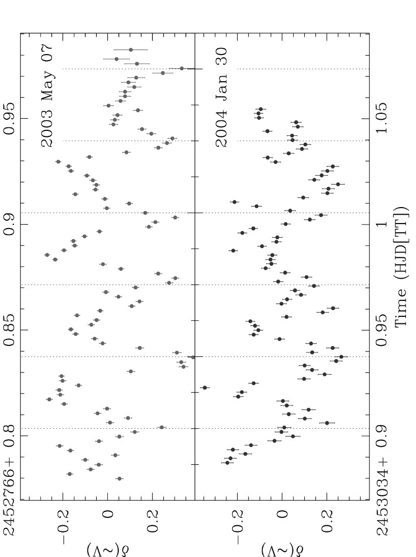
Figure 2.— The NOFS $\sim$$V$ lightcurves from the two different observations of SDSS J1446+02 are plotted using a common time-scaling. We also over-plot vertical bars to mark the length of each spin cycle; comparison of the variations during each successive spin cycle shows how much more regular they are in 2003 May 07 than in 2004 Jan 30; possibly enhanced flickering is responsible for the increased scatter in the latter curve.

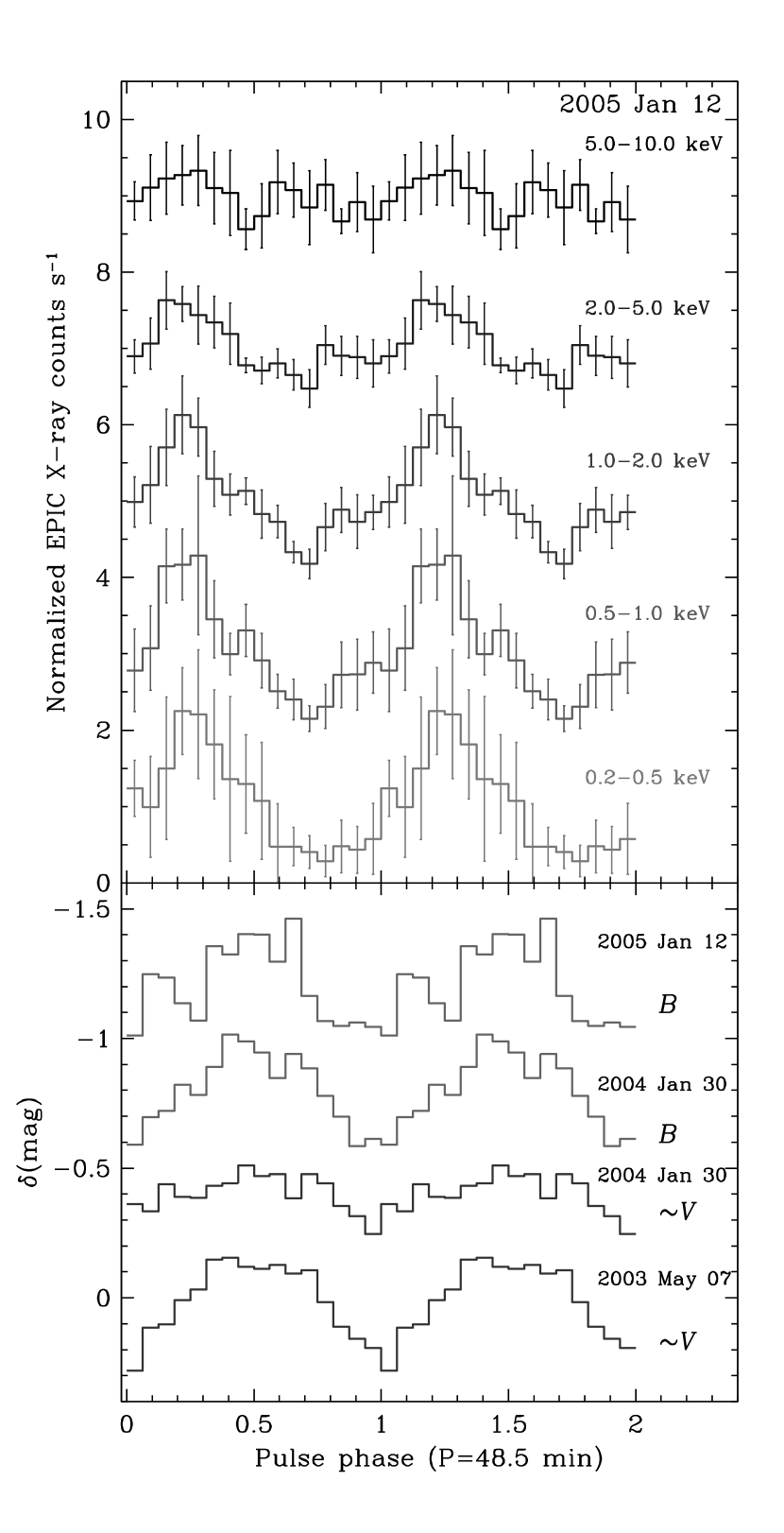
Figure 3.— White Dwarf spin phase folded, and binned light curves for SDSS J1446+02. Upper: the energy-selected EPIC X-ray light curves; note the marked change in amplitude, increasing with decreasing energy. Lower: the optical light curves from the two XMM-Newton/OM ( in $B$) and two NOFS observations (in an approximate $V$ band); in the NOFS light curves the change in amplitude, due to the variation in scatter about the mean curve is made very apparent. Note: (i) the simultaneous X-ray and OM 2005 Jan 12 lightcurves share a common ephemeris, arbitarily chosen to place optical minimum at phase=0.0, the phasing of each of the other optical lightcurves has simply been chosen to align their optical minima; (ii) for clarity each of these lightcurves has been offset vertically, with 2 normalized X-ray counts and 0.4 mags respectively.

For SDSS J1446+02 we also possess four optical lightcurves (two from the ground and two from the OM), plus those from the EPIC X-ray cameras. To maximize signal-to-noise we summed the results from the two MOS; however, since these are always of longer duration than the pn, we did not combine pn and MOS at this stage. We performed a Lomb-Scargle periodogram (Scargle, 1982) analysis of each of our lightcurves. In every case, a significant peak was found at a period of 49 min, which we identify as the spin period of the white dwarf. In addition, longer term variations were apparent in the optical lightcurves with peaks corresponding to around 4 hrs, close to the signal found in the time-resolved APO spectra. To determine the periods most accurately, we used sinusoidal fitting to the longest 2003 May 7 NOFS lightcurve, with a sinusoid plus first harmonic model for the pulse, and a simple sinusoid for the longer period variation. This yielded a period of $0.0338\pm 0.004$d ($48.7\pm 0.5$ min) for the pulse, and $0.165\pm 0.015$d ($4.0\pm 0.4$hr) for the longer period, which we presume to be the orbital period of the system. Once again we caution that the 2003 May curve provides only 1.3 cycles coverage of our tentative orbital period, and it remains poorly constrained. Nevertheless, we then fit the other three optical curves with sinusoids constrained to the pulse and orbital periods, and subtracted the latter. In fig. 2 we show the two resulting NOFS lightcurves; the pulse profile is obvious in most cycles in the 2003 May curve, whereas in 2004 Jan there is far more scatter, especially away from minimum light. This may simply be due to varying amounts of flickering, perhaps indicative of small changes in accretion state. Lastly, we phase folded (and binned) the light curves on the pulse period to examine its profile in greater detail. The binned results are shown (along with the X-ray) in Fig. 3. The profile is clearly far from sinusoidal, having a relatively broad and flat-topped peak, and narrower V-shaped minimum.

Before phase-folding the X-ray data, we created five different energy selected lightcurves, in order to investigate any dependence of the pulse profile on energy. The final binned lightcurves shown in Fig. 3 were constructed by summing the folded and binned results for all three X-ray cameras to maximize signal-to-noise. Perhaps not too surprising, the profile of the X-ray pulse is very different from the optical, but it is noteworthy that the X-ray and optical are neither in phase nor anti-phased. Instead, the peak of the X-ray roughly leads that of the optical by $\sim$0.3 in phase. The X-ray pulse is also energy dependent, with the largest amplitude (and symmetrical peaked pulse) in the two lowest energy bins, the amplitude then decreases with energy, until above 5 keV there is no significant variation.

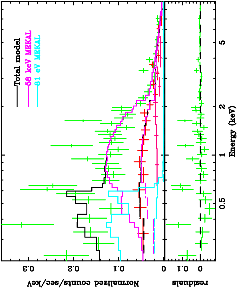
Figure 4.— Upper panel: XMM-Newton/EPIC-pn spectra for SDSS J1446+02 from the “max” (green or black points) and “min” (red or dark grey) spin phase intervals; the MOS data, used in the full joint fits, have been omitted for clarity. The best fit two temperature mekal  model is over-plotted for each (solid and dashed respectively); we also plot the two component contributions. Lower panel: the residuals to the fit of the total model.

3.2.2 Spectral variations with phase

The variation in pulse amplitude with energy is exactly that which we would expect if obscuration by a local absorber is responsible. In fitting the X-ray spectra, we first found a fit to the entire dataset, but then applied this model separately to spectra phase-selected from the maximum ($\phi=0.05-0.55$) and minimum ($\phi=0.55-1.05$) flux intervals of the pulse profile. The details of the fits are given in Table 2. The model that has the best fit consists of a two-temperature thermal plasma (mekal), absorbed both by a small Galactic column, but also by a much larger variable partial covering absorber. The fit to the combined spectrum achieved a barely acceptable reduced $\chi^{2}=1.1$ for 134 degrees of freedom (d.o.f.), though it does better than any other model. This model has a well-constrained cool plasma of $kT=130^{+2}_{-4}$eV contributing unresolved soft emission line structure plus a very hot component whose temperature pegged at 80 keV, the upper limit for the mekal model. Furthermore, the values of the Galactic and local columns were very poorly constrained. This is probably an effect of trying to fit a highly phase-variable spectrum with a single model (even this fairly complex one). Indeed, after separating the data into “max” and “min” subsets, a joint fit to these spectra was a significant improvement (see fig. 4). There was not a significant change in the reduced $\chi^{2}$, but we were now able to find well-constrained values for the absorbing columns and a physically plausible temperature for the hottest mekal component of $kT=58^{+22}_{-19}$keV. Once again the fit required a very cool mekal to account for line structure in the 0.3–0.4 keV range, plus O VII emission at 0.56 keV; indeed this parameter now pegged at its minimum value of 81 eV, indicating that some problems still remain (but the need for a very cool plasma is less problematic than an unphysically hot one, given the physical conditions in the expected complex multi-temperature accretion column). In this fit, the partial covering absorber parameters for the “max” tended to zero, hence we fixed them as such; the “min” interval as expected requires a thick column around $4\times 10^{22}$cm^-2, with 61% covering fraction. In our joint fit we found no statistical support for varying any of the normalization parameters; the change between “max” and “min” is entirely accounted for by the introduction of the thick partial covering absorber. Therefore, the fully unabsorbed flux (0.01–10 keV) remains constant at $3\times 10^{-11}\thinspace\hbox{$\hbox{erg}\thinspace\hbox{cm}^{-2}\thinspace\hbox{s}^{-1}$}$, whereas the affect of the absorption leads to clear energy-dependent changes in the observed fluxes: a drop of 60% ($4.6-1.8\times 10^{-13}\thinspace\hbox{$\hbox{erg}\thinspace\hbox{cm}^{-2}\thinspace\hbox{s}^{-1}$}$) in the softest 0.2–2.0 keV band; a decrease of only 30% ($7.6-5.6\times 10^{-13}\thinspace\hbox{$\hbox{erg}\thinspace\hbox{cm}^{-2}\thinspace\hbox{s}^{-1}$}$) in the 2.0–5.0 keV; and no significant change in the flux above 5 keV.

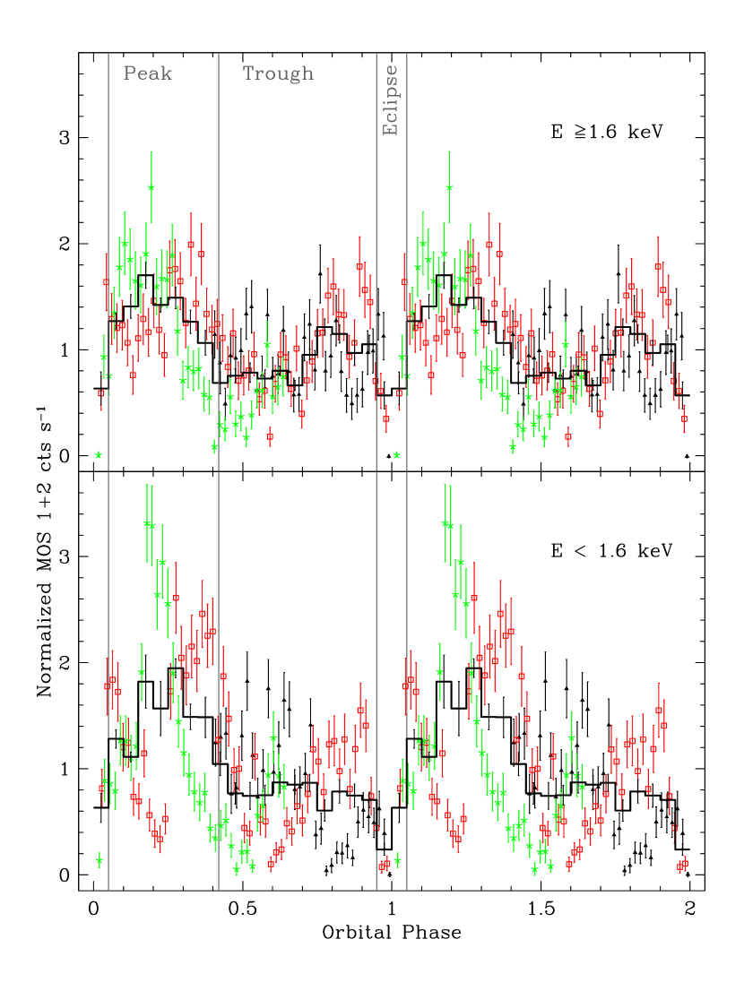
Figure 5.— Energy-selected XMM-Newton/EPIC-MOS (combined) X-ray lightcurves of SDSS J2050–05, phase-folded on our revised ephemeris: (top panel) a hard band with $E\geq 1.6$keV; (bottom panel) soft band with $E<1.6$ keV. Each of the three cycles covered is shown with a different symbol and grey shade (color in electronic edition) in order to show how much of the variability is apparently random flickering, and is more pronounced in the soft energy band. The average orbital modulation is brought out by binning the data; this curve is over-plotted in solid black. The vertical grey bars and labelling indicate the three phase intervals into which the data were subdivided to study variations in the spectra.

3.3. SDSS J2050–05

The eclipses seen in the optical photometry of Woudt et al. (2004) are also very apparent in the X-ray lightcurves, and in our $B$-band OM results. Their ephemeris is sufficiently precise that there is merely a 0.01 cycle uncertainty at the time of our XMM-Newton observations. Adding our own eclipse center measurements, we are able to even further refine the ephemeris to:

$${\rm HJD_{min}(TT)}=2453296.29816(6)+0.06542463(1)\ast E\;\;\;{\rm d}$$

where the numbers in parenthesis indicate the $1\sigma$ uncertainty in the last digit. Also, note that the time is given in Terrestrial time (UT=TT+64.184 s at the present epoch).

Besides the eclipses, the X-ray lightcurves exhibit large amplitude but apparently irregular flaring behaviour. We divided the X-ray data into two energy bins, above and below 1.6 keV, roughly encompassing the same count rates, then phase-folded the lightcurves and we plot them in fig. 5, where we also plot each cycle of data with a different symbol (and color in the electronic edition). Although this energy division is not physically motivated, it does roughly separate the energies severely affected by photo-electric absorption from those little affected (as can been seen in fig. 6). We note, however, that the soft band does include contributions from physically distinct X-ray emission regions– the heated white dwarf surface, and the accretion column– which should be borne in mind in any interpretations of the lightcurves. We see that the flaring does not repeat in each orbit, and that it is far more significant below 1.6 keV. The over-plotted binned data (stepped line) bring out the average orbital modulations more clearly. At the higher energies, there appears to be a broad peak, cut unevenly by the eclipse, whereas at lower energies, the rise in flux to peak does not occur until phase 0. As we did for SDSS J1446+02, we undertook X-ray spectral fitting to both the complete dataset, and two phase-selected intervals, here dubbed “peak” and “trough”, excluding the eclipse phase: these regions are also indicated in fig. 5.

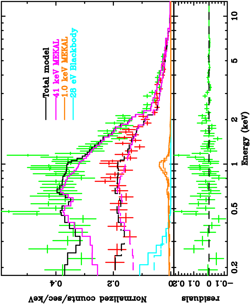
Figure 6.— Upper panel:XMM-Newton/EPIC-pn spectra for SDSS J2050–05 from the “peak” (black or green points) and “trough” (red or dark grey) orbital phase intervals; the MOS data, used in the full joint fits, have been omitted for clarity. The best fit two temperature mekal plus blackbody model is over-plotted for each (solid and dashed respectively); we also plot the various component contributions. The hotter emitting gas provides the dominant contribution, and the change in overall flux between the intervals is due to a combination of its changing normalization and the extra absorption from a dense partial covering component. Lower panel: the residuals to the fit of the total model.

Table 3X-ray Spectral Fits for SDSS J2050–05

Model	reduced	$N_{H}$	Partial covering		$kT_{\rm BB}$	$kT$(s)
	$\chi^{2}$	$\times 10^{20}$	$N_{H}$	frac.	(eV)	(keV)
	(d.o.f.)	cm-2	($\times 10^{22}$cm-2)
bremss	0.99 (418)	$4.3\pm 0.3$	$\cdots$	$\cdots$	$\cdots$	$166^{+33}_{-40}$
mekal	1.01 (418)	$4.8\pm 0.3$	$\cdots$	$\cdots$	$\cdots$	$80^{+0}_{-5}$
2 $T$ mekal	1.00(416)	$7.4\pm 0.3$	$\cdots$	$\cdots$	$\cdots$	$(8.08^{+0.1}_{-0})\times 10^{-2}$
						$80^{+0}_{-17}$
BB + mekal	0.99 (416)	$5.7^{+0.5}_{-0.4}$	$\cdots$	$\cdots$	$20^{+8}_{-6}$	$80^{+0}_{-9}$
BB + bremss.	0.98 (416)	$5.6^{+0.4}_{-0.8}$	$\cdots$	$\cdots$	$22^{+1}_{-10}$	$100^{+32}_{-19}$
2 $T$ mekal + BB	0.99 (412)	$5.1^{+0.5}_{-0.7}$	$1.4^{+0.8}_{-0.6}$	$0.14^{+0.45}_{-0.05}$	$32^{+1}_{-5}$	$1.3^{+1.3}_{-0.5}$
						$59^{+21}_{-15}$
Joint fit to phase-selected “peak” and “trough” intervals:
2 $T$ mekal + BB	0.88 (417)	$4.9^{+0.5}_{-0.7}$	none (pk)	none (pk)	$28^{+10}_{-13}$	$1.0^{+0.3}_{-0.2}$
			$1.3^{+0.4}_{-0.3}$(tr)	$0.35\pm{+0.03}$(tr)		$41^{+5}_{-13}$

For the complete dataset acceptable fits (see Table 3) were found for two component models with Galactic absorption consistent with the maximum line-of-sight column, with a optically thin thermal component (hot bremsstrahlung or mekal equally) plus a soft blackbody. However, the temperature of the hotter component at $\sim$80 keV is higher than typically found in CVs. We then investigated the phase-selected spectra seeking a single model requiring the fewest varying parameters. The final model consists of a two-temperature thermal component plus a soft blackbody, with partial covering absorption. In the light of this success, we also fit the complete dataset with the same model; in all cases we found physically plausible temperatures and absorption columns. The dominant contribution to the observed absorbed flux (98% in 0.01–10 keV range) is from a hot mekal with kT$\approx 40$ keV, but $F-$tests confirm the importance of the soft blackbody to provide the softest X-ray flux (at 93% confidence), and the cool mekal to account for significant unresolved line emission at $\sim$1keV (98%). The change in the spectrum from peak to trough is in part due to increased partial covering absorption: the peak spectrum requires no absorption in excess of the Galactic column, while for the trough we find a 35% covering column with $N_{H}=1.3\times 10^{22}{\rm cm}^{-2}$; and also to a decrease by 25% in the normalization of the hot mekal; the blackbody and cool mekal normalizations remain unchanged. The fully unabsorbed 0.01–10 keV flux amounts to $5\times 10^{-12}\thinspace\hbox{$\hbox{erg}\thinspace\hbox{cm}^{-2}\thinspace\hbox{s}^{-1}$}$, with 40 percent contributed by the soft blackbody. In fig. 6 we show the fits to the phase-selected spectra, together with a break-down of the three components; for clarity we only show data from the pn, though we used pn and the two MOS spectra when fitting.

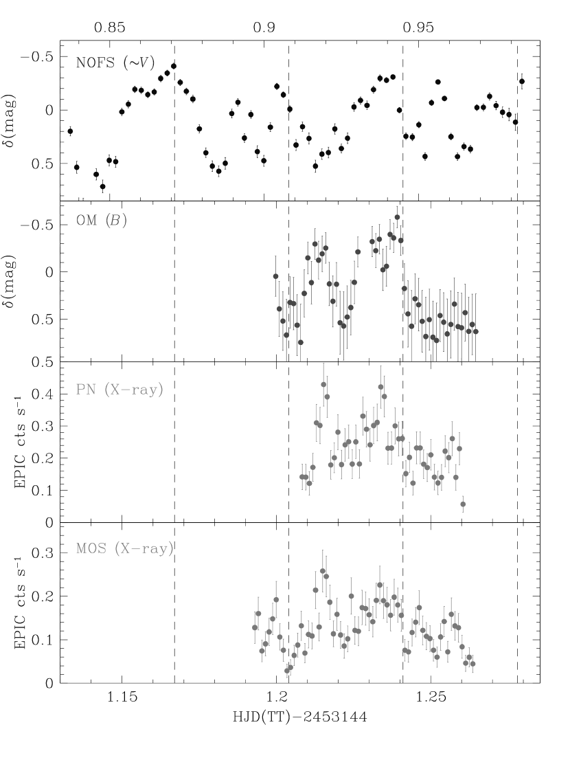
Figure 7.— Lightcurves for SDSS J2101+10 from NOFS (optical) and XMM-Newton (optical and X-ray). The lower three panels share a common time axis, while the earlier NOFS observation differs and is marked on the top axis. The vertical bars mark the times of (arbitrary) phase 0.0 and 0.5 for a 107 min period (detected in the NOFS lightcurve).

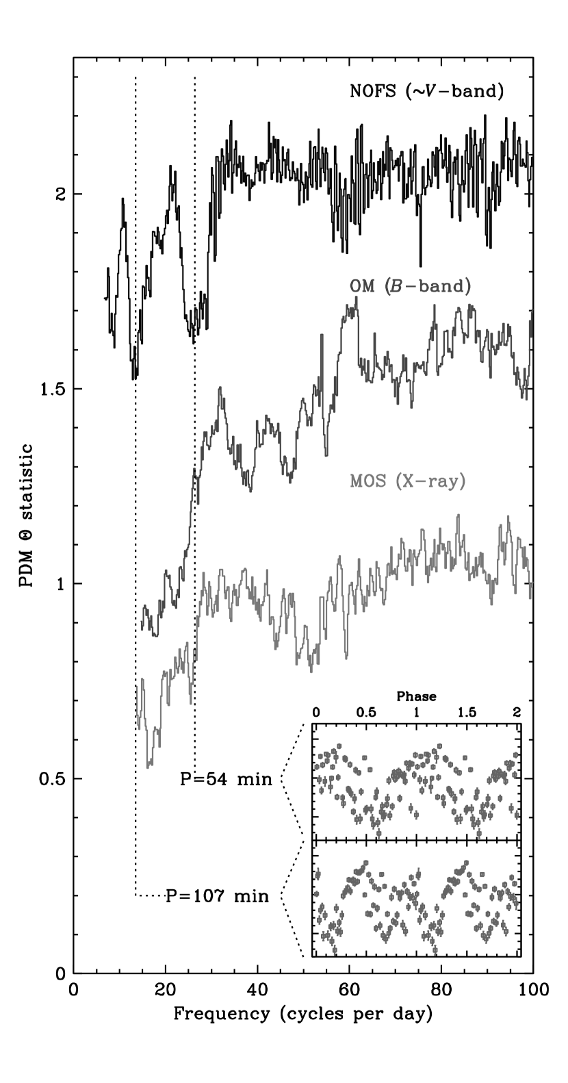
Figure 8.— Phase Dispersion Minimization periodograms for the MOS X-ray and NOFS and OM optical lightcurves of SDSS J2101+10. The successive curves have been offset vertically by 0.5 for clarity, and have been truncated at the low frequency end at the inverse of the respective lightcurve time span. The inset shows the NOFS lightcurve folded on its candidate periods, 54 and 107 min. The ordinate is in relative  $V$ magnitudes, with a 0.5 mag interval between large tick marks.

3.4. SDSS J2101+10

With no previously known periods, either spin or orbital, our first step was to examine the lightcurves (see fig. 7) for periodicities. Unfortunately, the XMM-Newton data span only $\sim$1.5 hr, and even the NOFS lightcurve is only 3.5 hrs long, limiting our sensitivity to any modulations with periods much in excess of 2 hours. Moreover, the variability in both X-ray and optical bands appears extremely complex. The longest, NOFS optical, curve appears to show two distinct humps at around 0.87 and 0.94 (truncated HJD(TT)), but of course even here only two cycles are present. Running a phase dispersion minimization (PDM, Stellingwerf, 1978) period-folding search on this light curve, we find three signals, but the lowest frequency one is close to the inverse of the data time span, and is therefore unreliable. This leaves minima at around 13.5 d^-1 (107 min) and 26.4d^-1 (55 min), which are close to being harmonically related to each other. In figure 8 we show the PDM for the NOFS lightcurve and the lightcurve folded on the two candidate periodicities. The fold on the longer period confirms the repeatability of the aforementioned humps: only at phases (arbitrary) 0.25–0.5 do the two cycles agree; but the fold is also somewhat double-humped, with possibly a second interval of higher flux at around 0.9, although here there is a large amount of scatter. Folding on 54 min the points line up along an approximately sinusoidal curve, but again there is significant scatter about this mean at all phases. Furthermore, for this shorter period we can usefully interrogate the OM and MOS light curves: their PDMs are also plotted in fig. 8; no strong signals appear around 54 min.

Table 4X-ray Spectral Fits for SDSS J2101+10

Model	reduced	$N_{H}$	$kT_{1}$ or	$kT_{2}$ (keV)
	$\chi^{2}$ (d.o.f.)	$\times 10^{20}$cm-2	$kT_{\rm max}$(keV)	or $\alpha$
mekal	0.82 (95)	7.1 (fixed)	$9\pm 1$	$\cdots$
mekal	0.80 (94)	$8.4^{+1.4}_{-0.7}$	$8\pm 2$	$\cdots$
2 $T$ mekal	0.77 (92)	$8.6^{+1.2}_{-1.1}$	$9.5^{+3.2}_{-1.6}$	$1.0\pm 0.2$
multi-$T$ mekal	0.75 (93)	$8.6^{+1.4}_{-0.9}$	$25^{+4}_{-5}$	$1.2^{+0.4}_{-0.2}$

Returning to fig. 7: in order to consider the NOFS periods further we have over-plotted vertical bars to mark phase 0.0 and 0.5 of a 107 min period, arranging the time axes for the XMM-Newton and NOFS observations to yield phase agreement (only 4 cycles elapse between the two sets of observations). We see that the repeatable NOFS humps agree in phase and approximate form with a hump in the OM lightcurve. However, at other phases agreement is lost, in particular another peak precedes the major hump in the OM, possibly correlated with a similar X-ray peak in fact. Ignoring the high frequency flickering in the X-ray lightcurves, there is possibly a slower variation on the $\sim$100 min timescale, though of course we have no way to test whether this behaviour actually repeats.

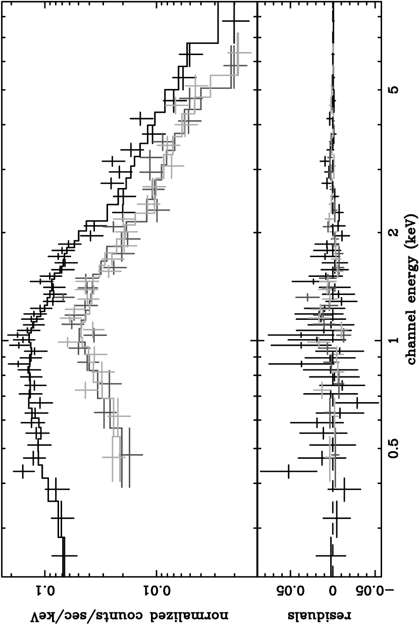
Figure 9.— XMM-Newton/EPIC spectra (points) and best fit model (line) for SDSS J2101+10: black–pn; dark grey–MOS1; light grey–MOS2. This model consists of a multi-temperature optically thin plasma model (cemekl), absorbed by $N_{H}=7.5\times 10^{19}$ cm^-2. In the lower panel the residuals to the fit are plotted.

In the absence of any decisive periods, we simply fit models to the complete X-ray spectrum. These are detailed in Table 4. A range of emission components from a single fairly cool mekal ($kT=9$keV), to a multi-temperature version with $kT_{\rm max}=25$keV provide adequate fits, all with a single absorbing component with $N_{H}\approx 8\times 10^{20}$cm^-2 consistent with the Galactic line-of-sight maximum. An example fit to the spectra is shown in fig. 9; the resulting unabsorbed 0.01–10 keV flux is $1.7\times 10^{-12}\thinspace\hbox{$\hbox{erg}\thinspace\hbox{cm}^{-2}\thinspace\hbox{s}^{-1}$}$.

4. Classifying the three sources

4.1. Nature of SDSS J1446+02

All the observational evidence indicates that SDSS J1446+02 is a short period IP. A classic signature of IPs is the presence of multiple periodicities in their lightcurves. For SDSS J1446+02 we find that both its optical and X-ray fluxes are strongly modulated at a short 49 min period, and there is evidence for an additional optical modulation at 4 hrs. This latter periodicity also appears in the H$\alpha$ radial velocity curve. However, more extensive photometric and spectroscopic runs are needed to confirm these, and hence secure the determination of the orbital period. The identification of the 49 min modulation with the spin period of an asynchronously rotating white dwarf is much more secure: the characteristic energy dependence of the X-ray flux modulation, and our simple phase-selected spectral fitting confirm that the variation in flux is dominated by changes in the local absorbing column. This is exactly as seen in many other IPs, as a result of the extended accretion curtain intersecting our line-of-site to the X-ray emitting accretion column.

The underlying X-ray emission can be fit with that emitted by a two-temperature optically thin plasma, i.e. bremsstrahlung. No doubt this simple model only approximates what must be a complex multi-temperature shock region in the accretion column, however the hotter component with $kT\approx 60$keV indicates the upper limit to the temperatures therein; again this value is typical of IPs.

Assuming that $P_{\rm orb}=4$hr, we find a ratio of $P_{\rm spin}/P_{\rm orb}=0.2$, placing SDSS J1446+02 well-within the group of so-called conventional IPs, as defined by $0.25>P_{\rm spin}/P_{\rm orb}>0.01$ and $P_{\rm orb}>4$hr (Norton et al., 2004). In all respects the observed properties of SDSS J1446+02 are consistent with a garden-variety IP.

4.2. Nature of SDSS J2050–05

The observational evidence favors a polar classification for SDSS J2050–05. One spectropolarimetric observation found significant circular polarization that increases to $v\sim 3\%$ for $\lambda>8000$ Å. This result suggests that the strongest cyclotron harmonics may lie in the near-IR, and thus that the magnetic field is relatively low, $B\mathrel{\hbox to0.0pt{\lower 3.0pt\hbox{$\mathchar 536\relax$}\hss}\raise 2.0pt\hbox{$\mathchar 316\relax$}}30$ MG, or that the specific accretion rate in the cyclotron-emitting portions of the funnel(s) is relatively low, $\dot{m}\mathrel{\hbox to0.0pt{\lower 3.0pt\hbox{$\mathchar 536\relax$}\hss}\raise 2.0pt\hbox{$\mathchar 316\relax$}}1$ g cm^-2, or both. No cyclotron harmonics are evident in either the total flux or circular polarization spectra, consistent with a high temperature shock. Therefore, SDSS J2050$-$05 is probably not a low-accretion rate polar (Schwope et al., 2002; Szkody et al., 2003b; Schmidt et al., 2005), where mass-transfer appears to occur not via Roche-lobe overflow, but rather by efficient magnetic capture of the secondary star’s stellar wind.

In support of the above interpretation, the X-ray spectra of SDSS J2050$-$05 are well-fit by a two-temperature thermal plasma model (mekal), but in addition the data require a soft blackbody component. In this case, the two mekal components have temperatures of 1 and 41 keV respectively, once again likely indicating the limits of the range of temperatures present in the optically thin emitting plasma, both quite typical for polars. The blackbody has a temperature of about 30 eV, again within the observed range for polars. In the “peak” region, this cool blackbody component, arising from the heated surface of the white dwarf, contributes about 40 percent of the unabsorbed 0.01-10 keV flux. In terms of the energy balance, assuming an X-ray albedo for the white dwarf surface of $a_{X}=0.3$ and that the cyclotron contribution to the energy losses is negligible, one finds $L_{\rm BB}/L_{\rm br}\approx\pi f_{\rm BB}(1-a_{X})d^{2}/2\pi f_{\rm br}(1+a_{X})d^{2}\approx 0.2$, which given uncertainties in estimating the unabsorbed soft flux is comparable to recent measures of the energy balance in other actively accreting polars.

As an eclipsing system, the orbital period is very well-established. In the X-ray lightcurves we again see eclipses, but the remainder of the variability is complex. It is dominated by aperiodic flickering behavior, which is strongest in the softer X-ray flux (below 1.6 keV). In an attempt to discover any underlying modulation on the orbital period, we created phase-binned light curves averaging over the three cycles of data. What remains appears quite typical of a polar, in which one accretion pole is always visible (i.e. no white dwarf self-eclipse). This produces emission modulated on the orbitally-synchronized white dwarf spin period, since the projected area of the emitting region changes with phase. The fact that only the normalization of the hotter thermal emission component appears to vary between “peak” and “trough” spectra is probably simply owing to poor statistics for the much smaller contributions from the cooler mekal and soft blackbody components. The shape of the average, non-eclipse harder X-ray ($E>1.6$keV) lightcurve is indeed approximately sinusoidal, whereas in the soft band the lightcurve does not rise until after the eclipse, i.e. its flux remains low in the phase range $\phi\approx 0.7-0.95$. The energy-dependence of this feature suggests that photo-electric absorption may be the cause. Indeed, the spectrum for the $\phi\approx 0.4-0.95$ “trough” phase interval does require a fairly high column, which partially covers the X-ray emission. Such pre-eclipse energy-dependent dipping structure is seen in many other eclipsing polars e.g. EP Dra, HU Aqr and UZ For (Ramsay et al., 2004; Schwope et al., 2001; Sirk & Howell, 1998). In the high-quality soft X-ray lightcurves of HU Aqr, there is one broad dip centered on phase 0.7 and a narrower feature at around 0.9. These are interpreted as arising from the accretion column obscuring the nearby heated photosphere of the white dwarf, while the more distant accretion stream accounts for the sharper dip, indeed the width and azimuth of this dip can be related to the geometry of the region where the stream threads onto the white dwarf’s magnetic field. Unfortunately, given the quality of our own data (both lacking the high signal-to-noise and afflicted by the flaring) we cannot identify the dipping components, and hence probe the accretion flow in greater detail; and of course from our spectral fitting we know that the soft flux arises both from the white dwarf and various parts of the accretion column, which would further complicate a more detailed analysis.

4.3. Nature of SDSS J2101+10

Although originally identified as a candidate mCV, given the strength of its high-excitation optical emission lines, the follow-up observations of SDSS J2101+10 we have presented do not seem to confirm this classification. We find no strong modulation of its X-ray flux, quite unlike any polar, for instance SDSS J2050–05. The X-ray spectrum also does not require any absorption in excess of the estimated Galactic column, effectively ruling out a typical IP. The X-ray emission is describable by a variety of thermal plasma (mekal) models, though with a noticeably lower maximum temperature ($kT\approx 10$ or at most 25 keV) than is found in most mCVs or indeed in our fits to SDSS J1446+02 or SDSS J2050–05. This cooler plasma is in fact far more typical of disk-accreting systems. Only the SW Sex stars show He II with strength comparable to the magnetics; both the lack of absorption in the line profiles and their barely detectable radial velocities could be accounted for by a low inclination to our line-of-sight.

5. Conclusions

We have reported on observations allowing classification of three new SDSS CVs showing prominent He II: SDSS J1446+02, SDSS J2050–05 and SDSS J2101+10. Each represents a different class of CV, known to exhibit such high excitation emission lines.

SDSS J1446+02 is a clear example of an IP. We find two periodicities at about 4 hr and 49 min, arising respectively from the orbit and asynchronously spinning white dwarf. The X-ray spectrum comprises a multi-temperature thermal plasma, with a maximum of 60 keV, modulated by phase-dependent local absorption. This likely originates from obscuration by the accretion curtains formed by the accreting material as it flows between the disrupted disc and the magnetic poles of the white dwarf.

SDSS J2050–05 represents the most highly magnetized of the three, a fully spin-orbit synchronized polar, with an orbital period of 1.57 hr. In this case no disk forms, and all accretion is channeled along the field lines to a single dominant pole. Owing to its high inclination, there is a phase interval when the accretion stream obscures the X-ray emitting region, but most of the modulation on the spin/orbit appears consistent with simply its changing aspect. The X-ray emission has two components: the dominant one is characteristic of the post-shock bremsstrahlung-cooled optically thin plasma of the accretion column, here with temperatures ranging from 1 keV to 40 keV; this also heats the surface of the white dwarf leading to additional soft blackbody (30 eV) emission.

In SDSS J2101+10, we suggest that the combination of high accretion rate and lower magnetic field strength allows disk-mediated accretion, but also the formation of He II emission lines in the optical spectra, i.e. if it were at higher inclination it would appear as a classic SW Sex star. Its X-ray spectra indicate a rather cool thermal plasma ($\sim$10 keV) more typical of disk systems, and an unobscured line of sight, inconsistent with an IP. From only weak modulation (unlike a polar) of its X-ray and optical lightcurves we suggest an orbital period in the 100 min range.

References

- den Herder et al. (2001) den Herder, J. W. et al. 2001, A&A, 365, L7
- Norton et al. (2004) Norton, A., Somerscales, R., & Wynn, G. 2004, in Magnetic Cataclysmic Variables: Proceedings of IAU Colloquium 190, ed. M. Cropper & S. Vrielmann, ASP Conf. Ser., in press
- Ramsay et al. (2004) Ramsay, G., Bridge, C. M., Cropper, M., Mason, K. O., Córdova, F. A., & Priedhorsky, W. 2004, MNRAS, 354, 773
- Rodríguez-Gil et al. (2001) Rodríguez-Gil, P., Casares, J., Martínez-Pais, I. G., Hakala, P., & Steeghs, D. 2001, ApJ, 548, L49
- Scargle (1982) Scargle, J. D. 1982, ApJ, 263, 835
- Schmidt et al. (1992) Schmidt, G. D., Stockman, H. S., & Smith, P. S. 1992, ApJ, 398, L57
- Schmidt et al. (2005) Schmidt, G. D. et al. 2005, ApJ, 630, 1037
- Schwope et al. (2002) Schwope, A. D., Brunner, H., Hambaryan, V., & Schwarz, R. 2002, in ASP Conf. Ser. 261: The Physics of Cataclysmic Variables and Related Objects, ed. B. T. Gänsicke, K. Beuermann, & K. Reinsch, 102
- Schwope et al. (2001) Schwope, A. D., Schwarz, R., Sirk, M., & Howell, S. B. 2001, A&A, 375, 419
- Shafter (1983) Shafter, A. W. 1983, ApJ, 267, 222
- Sirk & Howell (1998) Sirk, M. M. & Howell, S. B. 1998, ApJ, 506, 824
- Stellingwerf (1978) Stellingwerf, R. F. 1978, ApJ, 224, 953
- Strüder et al. (2001) Strüder, L. et al. 2001, A&A, 365, L18
- Szkody et al. (2003a) Szkody, P. et al. 2003a, AJ, 126, 1499
- Szkody et al. (2003b) Szkody, P. et al. 2003b, ApJ, 583, 902
- Turner et al. (2001) Turner, M. J. L. et al. 2001, A&A, 365, L27
- Warner (1995) Warner, B. 1995, Cataclysmic Variable Stars (Cambridge University Press), 57
- Wickramasinghe & Ferrario (2000) Wickramasinghe, D. T. & Ferrario, L. 2000, PASP, 112, 873
- Woudt et al. (2004) Woudt, P. A., Warner, B., & Pretorius, M. L. 2004, MNRAS, 351, 1015
- York et al. (2000) York, D. G. et al. 2000, AJ, 120, 1579