The DWT Power Spectrum of the two-degree Field Galaxy Redshift Survey

Abstract

The power spectrum of the two-degree Field Galaxy Redshift Survey (2dFGRS) sample is estimated with the discrete wavelet transform (DWT) method. The DWT power spectra within $0.04<k<2.3h$Mpc^-1 are measured for three volume-limited samples defined in connective absolute magnitude bins $-19\sim-18$, $-20\sim-19$ and $-21\sim-20$. We show that the DWT power spectrum can effectively distinguish $\Lambda$CDM models of $\sigma_{8}=0.84$ and $\sigma_{8}=0.74$. We adopt maximum likelihood method to perform three-parameter fitting with bias parameter $b$, pairwise velocity dispersion $\sigma_{pv}$ and redshift distortion parameter $\beta=\Omega_{m}^{0.6}/b$ to the measured DWT power spectrum. Fitting results denotes that in a $\sigma_{8}=0.84$ universe the best fitted $\Omega_{m}$ given by the three samples are consistent in the range $0.28\sim 0.36$, and the best fitted $\sigma_{pv}$ are $398^{+35}_{-27}$, $475^{+37}_{-29}$ and $550\pm 20$km/s for the three samples, respectively. However in the model of $\sigma_{8}=0.74$, our three samples give very different values of $\Omega_{m}$. We repeat the fitting by using empirical formula of redshift distortion. The result of the model of low $\sigma_{8}$ is still poor, especially, one of the best value $\sigma_{pv}$ is as large as $10^{3}$km/s. The power spectrum of 2dFGRS seems in disfavor of models with low amplitude of density fluctuations.

1 Introduction

The present clumpy structures indicated by galaxies on large scales are evolved from the very small density fluctuations in the early era of the universe. The amplitude of the fluctuation is fundamental to understand the structure formation. A remarkable success of modern cosmology is that the amplitude of mass fluctuations detected by the anisotropy of cosmic microwave background radiation is in excellent agreement with the analysis of the galaxy clustering at low redshifts. Recently released WMAP third year data (WMAP3) refines most results of cosmological parameters given by the WMAP 1st year data. However, the fluctuation amplitude smoothed in a spherical top hat window of radius of $8\rm{h^{-1}Mpc}$ is found as small as $\sigma_{8}=0.74^{+0.05}_{-0.06}$ (Spergel et al., 2006), which is significantly lower than $\sigma_{8}=0.84\pm 0.04$ of the WMAP 1st year data. The new result of $\sigma_{8}$ is a challenge to the cosmological parameter determinations from samples of galaxies and galaxy clusters, most of which yield $\sigma_{8}\simeq 0.9-1$ if the matter content of the universe $\Omega_{m}\leq 0.3$ (e.g. Reiprich & Böhringer, 2002; Hoekstra et al., 2002; Refregier et al., 2002; Van Waerbeke et al., 2002; Bacon et al., 2003; Bahcall & Bode, 2003; Seljak et al., 2005; Viel & Haehnelt, 2006).

The problem motivates us to revisit the constrains on $\sigma_{8}$ from the power spectrum of the sample of the two-degree Field Galaxy Redshift Survey (2dFGRS). The final released spectroscopic catalog of the 2dFGRS contains 221414 galaxies with good redshift quality $Q\geq 3$ and covers approximately 1800 square degrees of the sky. It is a good sample for studying the fluctuations of cosmic mass field on large scales in linear regime as well as on scales in nonlinear range. Moreover, the 2dFGRS team has made detailed analysis of the Fourier power spectrum, the two point correlation functions and relevant cosmological parameter fitting (Percival et al., 2001; Norberg et al., 2001; Peacock et al., 2001; Norberg et al., 2001; Hawkins et al., 2003; Percival et al., 2004; Cole et al., 2005). They found that $\Omega_{m}\sim 0.3$ or less (Peacock et al., 2001; Cole et al., 2005), and the best fitting value of $\sigma_{8}$ is $\sim 0.95$ if one takes $\Omega_{m}\sim 0.3$ (Percival et al., 2004), which is substantially different from WMAP3.

In the linear regime $\sigma_{8}$ only controls the overall amplitude of the power spectrum, and it is degenerated with the linear bias parameter $b$. Power spectrum on small scales is more effective to constrain $\sigma_{8}$ than on large scales since the nonlinearity of the power spectrum is directly reflected by the value of $\sigma_{8}$. Most measurements of the 2dFGRS power spectrum are on scales of $k<1h$Mpc^-1 while cosmological parameter estimation is performed on scale of $k<\sim 0.2h$Mpc^-1 (Peacock et al., 2001; Percival et al., 2001; Tegmark et al., 2002; Cole et al., 2005). With the estimator based on the discrete wavelet transformation (DWT) (Yang et al., 2001, 2001a, 2001b, 2002), we are to analyze the power spectrum of the 2dFGRS sample on scales down to $k\simeq 2h$Mpc^-1. In this scale range, the redshift distortion of DWT diagonal mode power spectrum can be easily approximated and the aliasing effect is exactly eliminated by the DWT algorithm (Fang & Feng, 2000).

The paper is organized as follows. In Section 2, the DWT power spectrum estimator is briefly introduced. Section 3 describes the construction of samples. The Section 4 demonstrates robustness and accuracy tests on the DWT power spectrum estimator. Section 5 lists our fitting results. Conclusions are stated in Section 6.

2 DWT Power Spectrum Estimator

The method of measuring galaxy power spectrum with the multi-resolution analysis of discrete wavelet transformation has been developed in the last decade (e.g. Pando & Fang, 1995, 1996; Fang & Feng, 2000; Yang et al., 2001b, 2002; Zhan & Fang, 2003). A brief summary of the method is given here, more details are written in the Appendix.

2.1 DWT Power Spectrum

The observed galaxy number density distribution is

$$n_{g}({\bf x})=\sum_{m=1}^{N_{g}}w_{m}\delta^{D}({\bf x-x}_{m})\ ,$$ (1)

where $N_{g}$ is the total number of galaxies, ${\bf x}=(x_{1},x_{2},x_{3})$ is a 3-dimensional position vector, ${\bf x}_{m}$ is the position of the $m^{th}$ galaxy, $w_{m}$ is its weight, and $\delta^{D}$ is the 3-D Dirac $\delta$ function. For an observed sample, $n_{g}({\bf x})$ can be regarded as a realization of a Poisson point process with intensity $n({\bf x})=\bar{n}_{g}({\bf x})[1+\delta({\bf x})]$, where $\bar{n}_{g}({\bf x})$ is selection function, and $\delta({\bf x})$ is the density contrast.

In terms of the DWT decomposition, the galaxy field is described equivalently by variables defined as

$$\tilde{\epsilon}_{\bf j,l}=\int\delta_{g}({\bf x})\psi_{\bf j,l}({\bf x})d{\bf x}\ ,$$ (2)

where $\delta_{g}({\bf x})=[n_{g}({\bf x})/\bar{n}_{g}({\bf x})]-1$, and $\psi_{\bf j,l}({\bf x})$ is the basis of the DWT decomposition, where index ${\bf j}=(j_{1},j_{2},j_{3})$ stands for the scale, and ${\bf l}=(l_{1},l_{2},l_{3})$ for position (see Appendix A). Since the orthogonal-normal bases $\psi_{\bf j,l}({\bf x})$ are complete, all second order statistical behavior of the field can be described by $\langle\tilde{\epsilon}_{\bf j,l}\tilde{\epsilon}_{\bf j^{\prime},l^{\prime}}\rangle$. The goal of power spectrum measurement is to estimate the power spectrum of the density fluctuations $\delta({\bf x})=[n({\bf x})/\bar{n}({\bf x})]-1$ from the observed realization $\delta_{g}({\bf x})=[n_{g}({\bf x})/\bar{n}_{g}({\bf x})]-1$. It has been shown in Fang & Fang (2006, hereafter paper I) that the power of the fluctuations on the modes with the scale index ${\bf j}$ can be estimated by

$$P_{\bf j}=I_{\bf j}^{2}-N_{\bf j}\ ,$$ (3)

in which

$$I_{\bf j}^{2}=\frac{1}{2^{j_{1}+j_{2}+j_{3}}}\sum_{l_{1}=0}^{2^{j_{1}}-1}\sum_{l_{2}=0}^{2^{j_{2}}-1}\sum_{l_{3}=0}^{2^{j_{3}}-1}[\tilde{\epsilon}_{\bf j,l}]^{2}\ ,$$ (4)

and

$$N_{\bf j}=\frac{1}{2^{j_{1}+j_{2}+j_{3}}}\sum_{l_{1}=0}^{2^{j_{1}}-1}\sum_{l_{2}=0}^{2^{j_{2}}-1}\sum_{l_{3}=0}^{2^{j_{3}}-1}\int\frac{\psi_{\bf j,l}^{2}({\bf x})}{\bar{n}_{g}({\bf x})}d{\bf x}\ .$$ (5)

The term $I_{\bf j}^{2}$ is the mean power of ${\bf j}$ modes measured from the observed realization $n_{g}({\bf x})$, and $N_{\bf j}$ is the power on ${\bf j}$ modes due to the Poisson noise. For a volume-limited survey, the mean galaxy density $\bar{n}_{g}$ is independent of the redshift. The Poisson noise power is thus simply $1/\bar{n}_{g}$. $P_{\bf j}$ is usually referred to as the DWT power spectrum.

The DWT power spectrum $P_{\bf j}$ is related to Fourier spectrum $P(n_{1},n_{2},n_{3})$ by

$$P_{\bf j}= \frac{1}{2^{j_{1}+j_{2}+j_{3}}}\sum_{n_{1}=-\infty}^{\infty}\sum_{n_{2}=-\infty}^{\infty}\sum_{n_{3}=-\infty}^{\infty}$$ (6)

$$|\hat{\psi}(n_{1}/2^{j_{1}})\hat{\psi}(n_{2}/2^{j_{2}})\hat{\psi}(n_{3}/2^{j_{3}})|^{2}P(n_{1},n_{2},n_{3})\ ,$$

where $\hat{\psi}(n)$ is the Fourier transform of the basic wavelet $\psi(x)$. Since $|\hat{\psi}(n)|^{2}$ is a high pass filter in the wavenumber space, $P_{\bf j}$ is banded Fourier power spectrum. If the cosmic density field is isotropic, the Fourier power spectrum $P(n_{1},n_{2},n_{3})$ depends only on $n=\sqrt{n_{1}^{2}+n_{2}^{2}+n_{3}^{2}}$. Eq.(6) are exact for homogeneously random fields, either Gaussian or non-Gaussian.

2.2 DWT algorithm of redshift-distortion

The DWT power spectrum depends on the scale and shape of the DWT mode $\psi_{\bf j,l}({\bf x})$, it is sensitive to distortion of the shape of the field. It is necessary to establish the mapping from the redshift space to the real space. The mapping is attributed to bulk velocity and pairwise peculiar velocity. In the linear treatment of bulk velocity, the redshift-distorted DWT power spectrum, $P^{S}_{\bf j}$ is related to the real space power spectrum $P_{\bf j}$ by (Yang et al., 2002)

$$P^{S}_{\bf j}=b^{2}(1+\beta S_{\bf j})^{2}S^{PV}_{\bf j}P_{\bf j}\ ,$$ (7)

in which $\beta=\Omega_{m}^{0.6}/b$, $b$ is the linear bias parameter. $S_{\bf j}$ of Eq.(7) is the linear redshift distortion factor. For a cubic box of $L_{1}=L_{2}=L_{3}=L$,

$$S_{j_{1},j_{2},j_{3}}= \frac{1}{2^{j_{1}+j_{2}+j_{3}}}\sum_{n_{1},n_{2},n_{3}=\infty}^{\infty}\frac{n_{3}^{2}}{n_{1}^{2}+n_{2}^{2}+n_{3}^{2}}$$ (8)

$$\cdot|\hat{\psi}(n_{1}/2^{j_{1}})\hat{\psi}(n_{2}/2^{j_{2}})\hat{\psi}(n_{3}/2^{j_{3}})|^{2}\ .$$

For diagonal modes $j_{1}=j_{2}=j_{3}=j$, $S_{j,j,j}=\frac{1}{3}$. The factor $S^{PV}_{\bf j}$ in Eq.(7) is the pairwise velocity dispersion factor. In the plane-parallel approximation, if the direction $j_{3}$ is chosen to be the line of sight, we have $S^{PV}_{\bf j}=[s^{pv}_{\bf j}]^{2}$, with

$$s^{pv}_{j_{1},j_{2},j_{3}}=\frac{1}{2^{j_{3}}}\sum_{n_{3}=\infty}^{\infty}|\hat{\psi}(n_{3}/2^{j_{3}})|^{2}\exp[-\frac{\sigma^{2}_{pv}}{2}(\frac{2\pi n_{3}}{L})^{2}]\ .$$ (9)

Obviously, the factor $(1+\beta S_{\bf j})^{2}$ corresponds to the linear redshift distortion, and $S^{PV}_{\bf j}$ is the nonlinear redshift distortion caused by the pairwise velocity dispersion. Although Eq.(7) is given by the linear approximation of bulk velocity, N-body simulation points out that the mapping of Eq.(7) works well till scale $k\simeq 2h$Mpc^-1, also because $P_{\bf j}$ is weakly affected by non-linear clumps of the density field. In general for non-volume limited samples, selection function shall be taken into account to model redshift distortion which brings in high order correction to Eq.(7) (Yang et al., 2002).

3 Sample Construction

Table 1: Volume limited sub-samples of 2dFGRS.

$M_{b_{J}}-5\log_{10}h$	$z_{min}$	$z_{max}$	$d_{min}$	$d_{max}$	$N_{g}^{SGP}/N_{g}^{NGP}$	$\bar{n}(10^{-3}h^{3}{\rm Mpc}^{-3})$
-19 — -18	0.0205	0.087	61.2	255.7	9737/7811	8.393
-20 — -19	0.0320	0.129	95.2	374.9	19122/14390	5.102
-21 — -20	0.0495	0.186	146.6	532.9	14734/10202	1.330

Samples used in our analysis are constructed basically in the same way as that in Pan & Szapudi (2005). We create volume limited samples from the 2dFGRS spectroscopic catalog of the final data release (Colless et al., 2003), which contains 221414 galaxies with good redshift quality $Q\geq 3$ (Colless et al., 2001). We exclude the ancillary random fields, leaving the two major contiguous trunks: one near the South Galactic Pole (SGP) covering approximately $-37^{\circ}\negthinspace.5<\delta<-22^{\circ}\negthinspace.5$, $21^{\rm h}40^{\rm m}<\alpha<3^{\rm h}40^{\rm m}$ and the other around the North Galactic Pole (NGP) defined roughly by $-7^{\circ}\negthinspace.5<\delta<2^{\circ}\negthinspace.5$, $9^{\rm h}50^{\rm m}<\alpha<14^{\rm h}50^{\rm m}$. In order to get maximum number of galaxies while keep an uniform sampling rate to guarantee the fairness of our statistics, we try different values of completeness $f$ ($f$ is defined as the ratio of the number of galaxies with redshift to the total number of galaxies contained in the parent catalog): fields with completeness less than the chosen value is cut off, and fields with higher completeness is diluted to match the sampling rate. We find $f=0.738$ is the optimal value. The final parent samples are thus restricted by completeness $f>0.738$, and apparent magnitudes limits in photometric $b_{J}$ band with bright cut of $m_{b_{J}}=15$ and faint cut of median value of $\sim 19.3$ with some small variation specified by masks (Colless et al., 2003).

Volume limited sub-samples are built from the parent sample by selecting galaxies in specified absolute magnitude ranges. Absolute magnitudes are calculated with $k+e$ correction in Norberg et al. (2002). Our analysis focus on the three sub-samples defined in absolute magnitude $M_{b_{J}}$ bins of $-19\sim-18$, $-20\sim-19$ and $-21\sim-20$. Basic parameters of the three volume limited samples of 2dFGRS are summarized in Table 1 in which lists range of redshifts $z_{min}$-$z_{max}$, range of comoving distances $d_{min}$- $d_{max}$, numbers of SGP and NGP galaxies, and the mean densities $\bar{n}$. Comoving distances are calculated from redshifts $z$ in the $\Lambda$CDM universe with $\Omega_{\Lambda}=0.7$ and $\Omega_{m}=0.3$.

4 Numerical Tests of the DWT Power Spectrum Estimator

In this section, we will test the DWT power spectrum estimator with Poisson samples and samples from N-body simulation. Nine realizations of Poisson samples are produced in box with side $L=239.5$ h^-1Mpc with $256^{3}$ points. All the measured DWT power spectra of these samples are plotted in the top panel of Figure 1. To test the stability of the DWT estimator we calculate the diagonal DWT power spectrum, $P_{j,j,j}$ for each realization, and then computing their mean $\overline{P}_{j,j,j}$. $P_{j,j,j}/\overline{P}_{j,j,j}$ are shown in the bottom panel of Figure 1. We can see that at $j\leq 2$(i.e. scales larger than $119.75h$${}^{-1}\rm{Mpc}$), there are as large as 50% variances in the diagonal DWT power spectrum. Thus we will not use data points with $j\leq 2$. At small scales, or large $j$, the DWT estimator gives reliable results. This is because the aliasing effect is effectively suppressed in the DWT analysis (Fang & Feng, 2000).

Figure 1: $Top$: Diagonal DWT power spectra of nine realizations of Poisson samples. Each sample is generated in a box with size of $239.5$ h^-1Mpc and $256^{3}$ particles. The relation between $j$ and physical scale is $l=239.5/2^{j}$ h^-1Mpc. $Bottom$: Ratios of diagonal DWT power spectra of nine realizations of Poisson samples to their mean spectrum.

Then, in order to test the geometric effect of samples on estimation of the power spectrum, we cut one of the Poisson sample into three sheet-like sub-samples as $60.0\times 239.5\times 239.5$, $20.0\times 239.5\times 239.5$, and $20.0\times 60.0\times 239.5$ (h${}^{-1}\rm{Mpc})^{3}$. Furthermore, a fourth sub-sample is constructed from the $20.0\times 239.5\times 239.5$ (h${}^{-1}\rm{Mpc})^{3}$ sub-sample by cutting off three parallel cylinders with radius of 5.0, 10.0 and 20.0 $h^{-1}\rm{Mpc}$ respectively. In Figure 2, we plot the ratios of the DWT power spectra of each sub-sample to their parent random sample $P^{c}_{j,j,j}/P_{j,j,j}$. For $j=2$ and 3 (or on the scale of $239.5/2$ h${}^{-1}\rm{Mpc}$ and $239.5/2^{2}$ h${}^{-1}\rm{Mpc}$), the scatters in those spectra can be larger than $50\%$, and the ratios are randomly distributed with variance of the order of unity. Actually, such significant scatters result from small number of modes on $j\leq 3$. For $j>3$, differences between those spectra are negligible, the DWT power spectrum estimator is well independent of sample geometry on small scales.

Figure 2: The ratios of DWT power spectra of cutted Poisson sub-samples to the parent Poisson sample. The parent Poisson sample is generated in a box with size of $239.5$ h^-1Mpc, with $256^{3}$ points. The sub-samples are defined in box of $60.0\times 239.5\times 239.5h^{-1}$Mpc (dash-dot-dot line); $20.0\times 239.5\times 239.5h^{-1}$Mpc (dash line); $20.0\times 60.0\times 239.5h^{-1}$Mpc (dash-dot line); and $20.0\times 60.0\times 239.5h^{-1}$Mpc with three cylinders chopped (dot line).

To further test the reliability of the DWT power spectrum estimator, we measured the DWT power spectrum of the Virgo simulation which is of $\Lambda$CDM cosmology with $256^{3}$ particles in box of size $239.5h^{-1}$Mpc. Figure 3 compares the theoretical DWT power spectrum with that estimated from the simulation. The theoretical DWT power spectrum is calculated from Eq.(6) with nonlinear power spectrum from the accurate fitting formula of Smith et al. (2003). Clearly, the theoretical spectrum and measurements are in good agreement on scales less than $239.5/2^{4}\simeq 15h^{-1}$Mpc. The test shows that the DWT power spectrum estimator can perfectly recover the original power spectrum on small scales.

The final test is to measure the DWT spectrum of the Virgo sample in a cubic window of side $479.0h^{-1}$Mpc which is twice of the simulation box size. Theoretically the power at scale $j$ in the box of side $479.0h^{-1}$Mpc corresponds to that at scale $j-1$ in the box of side $239.5h^{-1}$Mpc. It is clearly seen in Figure 3 that the spectrum measured in the $479.0h^{-1}$Mpc box at $j$ exactly equals to that measured in the $239.5h^{-1}$Mpc at $j-1$. The DWT estimator is independent of the size of the window box. One can choose the size of box freely and put the sample in the box wherever one like. Note that the difference of spectra at $j=2,\ 3$ are greater than other data points. Therefore, in the following analysis of the 2dFGRS catalogs, the first two data points in our spectra are discarded.

Figure 3: DWT power spectrum of Virgo simulation sample. The dash line on the right is measured with the box size of 479.0 $h^{-1}\rm{Mpc}$. Shifting the right dash line by one unit along j-axis, we get the dash line on the left. The dot line is the power spectrum measured in box of size 239.5 $h^{-1}\rm{Mpc}$. The solid line is the nonlinear power spectrum from the formula of Smith et al. (2003) with $\Omega_{m}=0.3$, $\Omega_{\Lambda}=0.7$ and $\sigma_{8}=0.9$.

5 DWT power spectrum of 2dFGRS samples

5.1 The diagonal DWT power spectrum

To achieve the largest possible volume, the NGP and the SGP regions are measured together in a window box of size $1403.0h^{-1}$Mpc. The size of the window is sufficient to cover all three volume limited sub-samples. The filling factor of each sub-sample is $0.07\%$, $0.24\%$, and $0.68\%$ respectively.

To estimate error bars of the DWT power spectra, we created mock volume limited samples from the 22 mock galaxy catalogs which are extracted from the Hubble volume simulation . Details of mock catalogs are in Cole et al. (1998). The set of the mock samples used here is the LambdaCDM04. The 22 mock samples are filtered with the same selection criteria and masks as the real galaxy volume limited sub-samples. Error bars of the DWT power spectra of the three 2dFGRS sub-samples are approximated by the 1-$\sigma$ scattering of their mock samples.

Short noise is not directly calculated with Eq.(5). Instead, we produce a number of Poisson samples with the same geometry as our samples. Numbers of points in these Poisson samples are the same as the number of galaxies in the sample under analysis. 22 Poisson samples for each sub-sample allow us to estimate error bars for short noise subtraction. These error bars are incorporated into the final results of galaxy power spectra.

Figure 4: DWT power spectrum of 2dFGRS volume-limited samples and theoretical spectra. The size of the cubic box is 1403.0 $h^{-1}\rm{Mpc}$. The relation between $j$ and physical scale is $l=1403.0/2^{j}$ h^-1Mpc. The power at large scales are suppressed by random motion of galaxies. Due to cosmic variance, the error bars at $j=3$ is large. At $j=9$, Poisson noise leads to large error bars.

In Figure 4 we present the measured diagonal DWT power spectra of the three volume limited samples, together with two theoretical nonlinear spectra of flat $\Lambda\rm{CDM}$ model with parameters A.) $\Omega_{m}=0.3$, $\Omega_{\Lambda}=0.7$ and $\sigma_{8}=0.84$ (Model A), and B.) $\Omega_{m}=0.24$, $\Omega_{\Lambda}=0.76$ and $\sigma_{8}=0.74$ (Model B). The scale range is $0.035<k<2.2h$Mpc^-1.

5.2 The fitting of redshift distorted power spectrum

The differences between the power spectra of model predictions and the real data shown in Figure 4 are mainly due to redshift distortion and bias. We adopt Eq. (7) to fit the power spectrum of 2dFGRS samples with the nonlinear real space DWT power spectrum from Eq. (6) and the formula of Smith et al. (2003). We firstly use the 22 mock samples to estimate the correlation between the powers of different DWT modes. We construct a covariance matrix

$$\tilde{C}_{jj^{\prime}}=\frac{1}{N_{sim}}\sum_{I=1}^{N_{sim}}\Delta d^{I}_{j}\Delta d^{I}_{j^{\prime}}\ ,$$ (10)

where $N_{sim}=22$ and $\Delta d^{I}_{j}=d^{I}_{j}-\langle d_{j}\rangle$. The vector $d^{I}$ consists of elements $d^{I}_{j}=P^{I}_{j,j,j}$ with $j=3,...,9$, $P^{I}_{j,j,j}$ is the power spectrum from the $I$-th simulation, and $\langle d_{j}\rangle$ is the mean. We found that off-diagonal elements of the covariance matrices are always one order of magnitude smaller than diagonal elements. Actually it is a typical feature in the DWT analysis. The correlations between different modes are highly suppressed regardless the field is Gaussian or non-Gaussian (Feng & Fang 2005). The quasi-diagonalizing of the correlation matrix in the DWT decomposition has been extensively used for data compression. By virtue of this property, we can compute $\chi^{2}$ with diagonal elements only. Namely, we use the Chi-Square as our maximum likelihood estimator

$$\chi^{2}=\sum^{N}_{j=1}\frac{[P_{j}-P^{S}_{j}(a_{1},a_{2},a_{3}...)]^{2}}{\sigma_{j}^{2}}\ ,$$ (11)

in which $P_{j}$ is observation data and $P^{S}_{j}(a_{1},a_{2},a_{3}...)$ is the redshift-distorted power of model with parameters $(a_{1},a_{2},a_{3}...)$. We take the Reduced-Chi-Square, which is defined as $\chi^{2}_{d.o.f}=\chi^{2}/(N-M)$ where $(N-M)$ is the degree of freedom, as our final results shown in tables.

We aim at detecting the influence of $\sigma_{8}$ on the power spectrum. Two fiducial $\Lambda$CDM models are considered here: A. $\sigma_{8}=0.84$, and B. $\sigma_{8}=0.74$. We select the linear bias parameters $b$, redshift distortion parameter $\beta$ (or $\Omega_{m}$) and pairwise velocity variance $\sigma_{pv}$ as fitting parameters. Other parameters of model A and B are the same. The parameter space $(b,\beta,\sigma_{pv})$ is divided into a $20\times 20\times 20$ grid. The first run of fitting is performed on very crude grids in broad parameter space to locate the region of best $\chi^{2}$. Then we decrease the volume of parameter space centered in this region with finer grid to obtain the three dimensional probability distribution functions (PDF) of $(b,\beta,\sigma_{pv})$. After integrating over two of the three axes in the parameter space, we have the marginalized PDF for each parameter.

5.3 Fitting results

Table 2: Parameters estimated by fitting 2dFGRS DWT power spectra with Eq. (7) to $\Lambda\rm{CDM}$ model of $\sigma_{8}=0.84$.

$M_{b_{J}}-5\log_{10}h$	$\beta$ /$\Omega_{m}$	$b$	$\sigma_{pv}$ ($\rm{kms^{-1}}$)	$\chi^{2}$
-19 — -18	$0.66^{+0.06}_{-0.10}$ /$0.31^{+0.08}_{-0.12}$	$0.75^{+0.05}_{-0.06}$	$398^{+36}_{-27}$	8.87
-20 — -19	$0.62^{+0.07}_{-0.10}$ /$0.36^{+0.12}_{-0.14}$	$0.86^{+0.08}_{-0.07}$	$475^{+37}_{-29}$	16.19
-21 — -20	$0.43^{+0.02}_{-0.02}$ /$0.28^{+0.02}_{-0.02}$	$1.07^{+0.01}_{-0.01}$	$550^{+20}_{-20}$	4.06

Table 3: Parameters estimated by fitting 2dFGRS DWT power spectra with Eq. (7) to $\Lambda\rm{CDM}$ model of $\sigma_{8}=0.74$.

$M_{b_{J}}-5\log_{10}h$	$\beta$ /$\Omega_{m}$	$b$	$\sigma_{pv}$ ($\rm{kms^{-1}}$)	$\chi^{2}$
-19 — -18	$0.76^{+0.07}_{-0.09}$ /$0.41^{+0.10}_{-0.12}$	$0.77^{+0.05}_{-0.05}$	$415^{+40}_{-26}$	12.24
-20 — -19	$0.73^{+0.12}_{-0.10}$ /$0.46^{+0.20}_{-0.16}$	$0.86^{+0.09}_{-0.07}$	$492^{+38}_{-40}$	17.99
-21 — -20	$0.35^{+0.02}_{-0.02}$ /$0.28^{+0.02}_{-0.02}$	$1.19^{+0.01}_{-0.01}$	$600^{+15}_{-15}$	4.83

Table 4: Parameters estimated by fitting 2dFGRS DWT power spectra with Eq. (7) to the model of $\Omega_{m}=0.24$ and $\Omega_{\Lambda}=0.76$.

$M_{b_{J}}-5\log_{10}h$	$\sigma_{8}$	$b$	$\sigma_{pv}$ $\rm{kms^{-1}}$	$\chi^{2}$
-19 — -18	$0.43^{+0.20}_{-0.06}$	$0.99^{+0.20}_{-0.10}$	$490^{+42}_{-40}$	10.74
-20 — -19	$0.97^{+0.09}_{-0.06}$	$0.82^{+0.15}_{-0.13}$	$445^{+45}_{-35}$	16.83
-21 — -20	$0.94^{+0.04}_{-0.04}$	$0.99^{+0.09}_{-0.05}$	$505^{+40}_{-35}$	4.77

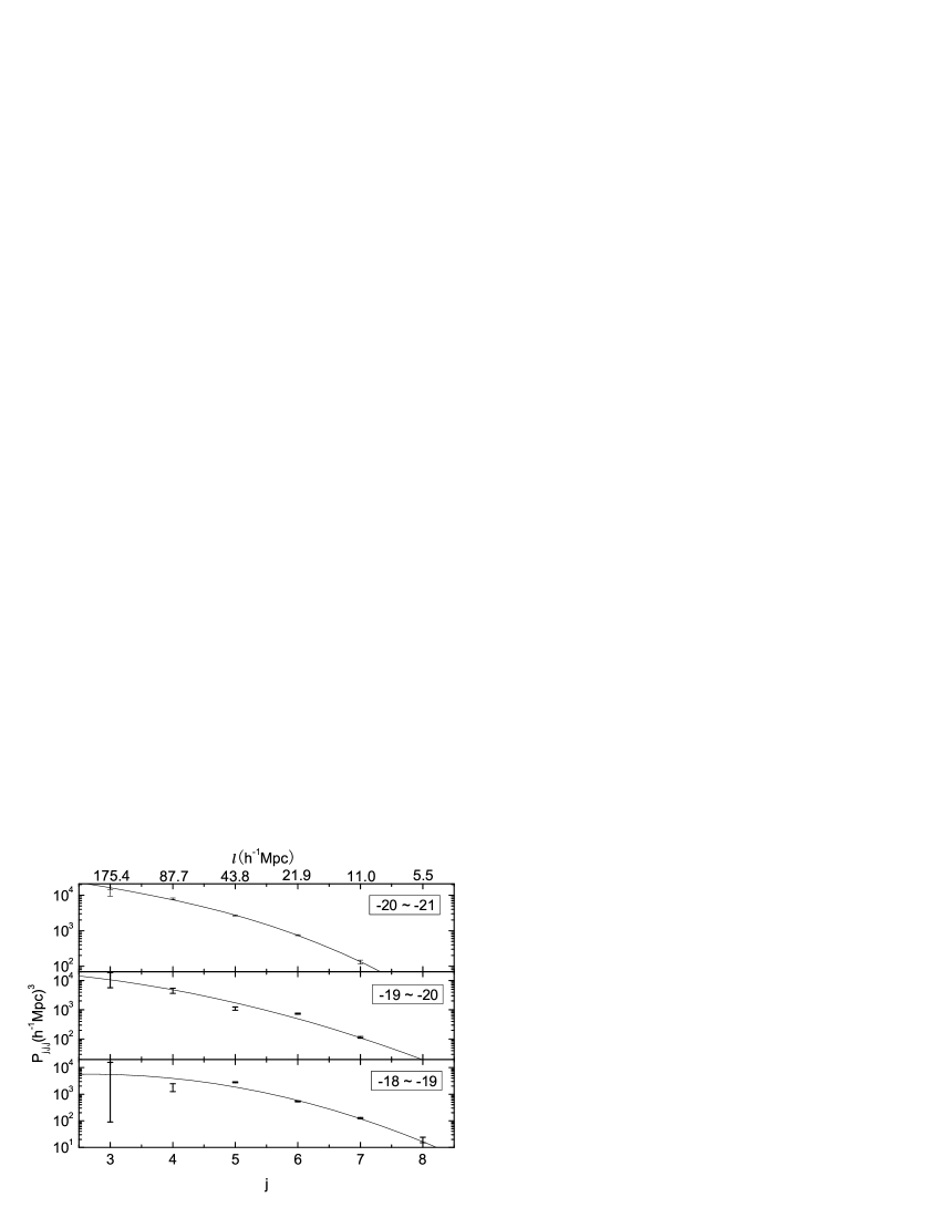
Figure 5: The DWT power spectra in redshift space of the $\rm{\Lambda CDM}$ model with $\sigma_{8}=0.84$. Parameters $b$, $\beta$, and $\sigma_{pv}$ are given by our best fitting to the data points shown in the Figure. The three panels are for sample within absolute magnitudes $-20\sim-21$ (top); $-19\sim-20$ (middle) and $-18\sim-19$ (bottom).

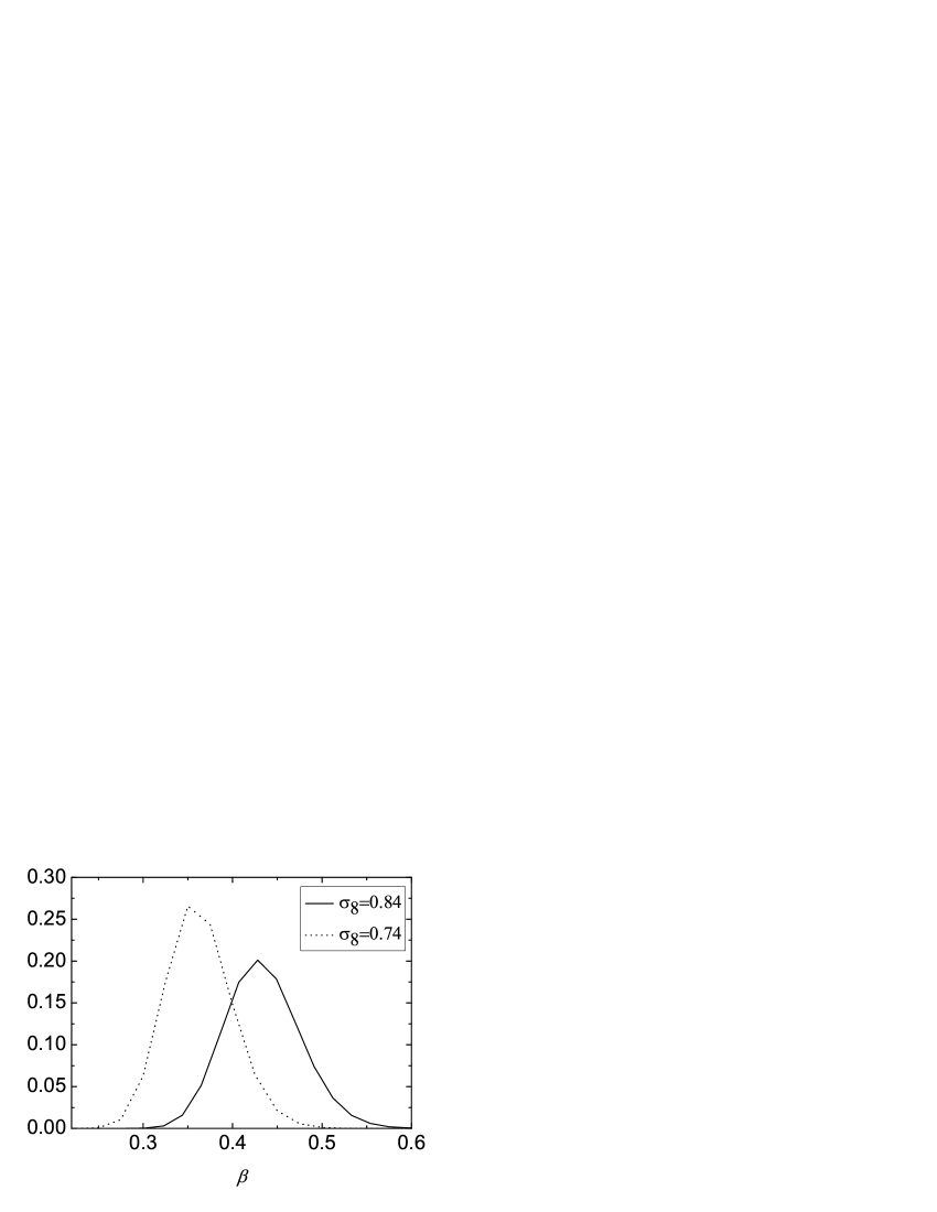
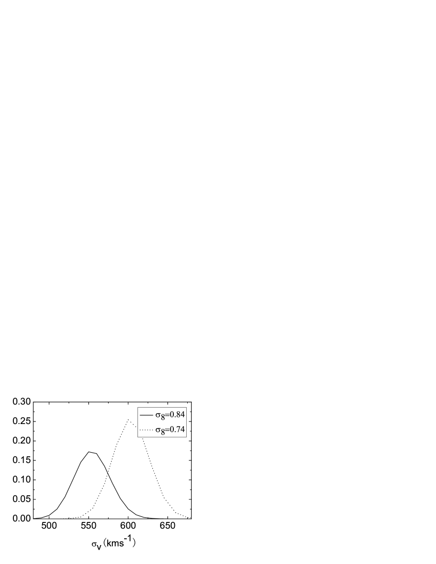
Figure 6: Marginalized distribution of parameters $b$, $\beta$, and $\sigma_{pv}$ in fitting the DWT power spectrum of the 2dFGRS sample of $M_{b_{J}}\in(-20\sim-21)$ with Eq. (7).

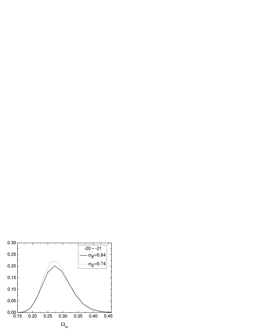
Figure 7: Marginalized distributions of $\Omega_{m}$ in fitting the DWT power spectra with Eq. (7) for 2dFGRS samples with $M_{b_{J}}$ in $-18\sim 19$, $-19\sim-20$ and $-20\sim-21$.

The best fitted power spectra of both models are very close to each other, so only the fitted power spectra of model A are demonstrated in Figure 5. The estimated parameters of the model A and B are tabulated in Tables 2 and 3 respectively. As an example, marginalized PDFs of the parameters $b,\beta,\sigma_{pv}$ for the sub-sample $-21\sim-20$ are in Figure 6. Figure 7 gives the PDFs of $\Omega_{m}$ for all the three sub-samples.

In Table 2 we can see that three sub-samples offer about the same estimation of $\Omega_{m}\simeq 0.3$, and the $b$ increases from $0.75$ to $\simeq 1$ with the luminosity of galaxies, which is consistent with analysis of others (Norberg et al., 2001; Pan & Szapudi, 2005). The pairwise velocities obtained in the three samples are in the reasonable range, and also increase with galaxy luminosity. It appears that our analysis with model A ($\sigma_{8}=0.84$) is basically in good agreement with previous works, and more importantly, that the DWT proves itself an effective tool for parameter estimation from galaxy samples.

Fitting to model B provides very different estimation of parameters. As seen in Table 3 and Figure 7, values of $\Omega_{m}$ given by the three sub-samples are quite different from each other. The best values of $\Omega_{m}$ for the sub-samples of $-19\sim-18$ and $-20\sim-19$ are significantly larger than $0.3$, which is in disagreement with most current measurements at least at 1-$\sigma$ level (e.g. Peacock et al., 2001; Tegmark et al., 2004). Only the sub-sample of $-21\sim-20$ yields the $\Omega_{m}\approx 0.3$.

In order to place constrains from the 2dFGRS on $\sigma_{8}$, we repeat the fitting procedure with $\sigma_{8}$, $b$ and $\sigma_{pv}$ as fitting parameters, and $\Omega_{m}=0.24$ as prior. Results are shown in Table 4. It is very clear that, except the $-19\sim-18$ sub-sample, the other two sub-samples both give $\sigma_{8}>0.9$. An universe of $\sigma_{8}=0.74$ is not preferred by the DWT power spectrum of the 2dFGRS.

5.4 Fitting with an alternative formula of redshift distortion

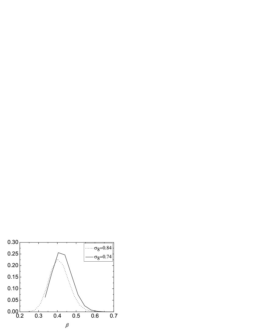
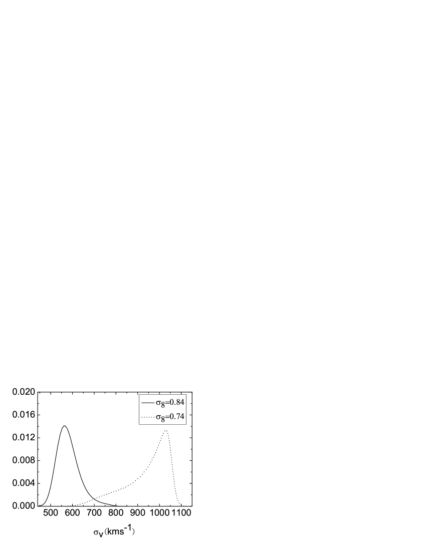
Figure 8: Marginalized distribution of parameters $\beta,b,\sigma_{pv}$ for the $-20\sim-21$ sub-sample, with the empirical redshift distortion mapping formula of Eq. (12). Fitting with $\sigma_{8}=0.74$ give larger $b$ and $\sigma_{pv}$ than with $\sigma_{8}=0.84$.

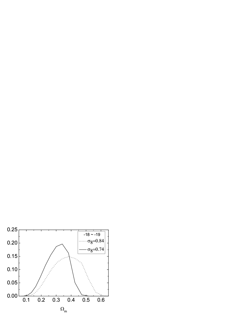
Figure 9: Marginalized distribution of $\Omega_{m}$ in three parameter fitting with Eq. (12). For all sub-samples, fitting with lower $\sigma_{8}$ gives larger value of $\Omega_{m}$.

Table 5: Best parameters from fitting DWT power spectra to $\Lambda\rm{CDM}$ model with $\sigma_{8}=0.84$ and Eq. (12).

$M_{b_{J}}-5\log_{10}h$	$\beta$ /$\Omega_{m}$	$b$	$\sigma_{pv}$ ($\rm{kms^{-1}}$)	$\chi^{2}$
-19 — -18	$0.77^{+0.08}_{-0.17}$ /$0.34^{+0.15}_{-0.20}$	$0.69^{+0.12}_{-0.09}$	$315^{+68}_{-44}$	10.91
-20 — -19	$0.73^{+0.06}_{-0.12}$ /$0.56^{+0.14}_{-0.22}$	$0.97^{+0.08}_{-0.07}$	$578^{+50}_{-40}$	8.46
-21 — -20	$0.41^{+0.07}_{-0.03}$ /$0.28^{+0.10}_{-0.05}$	$1.15^{+0.05}_{-0.03}$	$548^{+68}_{-26}$	4.96

Table 6: Best parameters from fitting DWT power spectra to $\Lambda\rm{CDM}$ model with $\sigma_{8}=0.74$ and Eq. (12).

$M_{b_{J}}-5\log_{10}h$	$\beta$ /$\Omega_{m}$	$b$	$\sigma_{pv}$ ($\rm{kms^{-1}}$)	$\chi^{2}$
-19 — -18	$0.76^{+0.08}_{-0.17}$ /$0.38^{+0.15}_{-0.20}$	$0.74^{+0.10}_{-0.07}$	$336^{+57}_{-41}$	10.61
-20 — -19	$0.73^{+0.06}_{-0.12}$ /$0.73^{+0.19}_{-0.27}$	$1.13^{+0.09}_{-0.07}$	$682^{+43}_{-41}$	8.26
-21 — -20	$0.40^{+0.06}_{-0.03}$ /$0.39^{+0.11}_{-0.07}$	$1.42^{+0.03}_{-0.06}$	$1014^{+51}_{-113}$	4.89

Table 7: Best parameters $\sigma_{8}$, $b$, $\sigma_{pv}$ from fitting DWT power spectra to $\Lambda\rm{CDM}$ model with $\Omega_{m}=0.24$, $\Omega_{\Lambda}=0.76$, and Eq. (12).

$M_{b_{J}}-5\log_{10}h$	$\sigma_{8}$	$b$	$\sigma_{pv}$$\rm{kms^{-1}}$	$\chi^{2}$
-19 — -18	$0.80^{+0.14}_{-0.08}$	$0.73^{+0.21}_{-0.12}$	$325^{+66}_{-50}$	17.00
-20 — -19	$0.93^{+0.10}_{-0.07}$	$0.91^{+0.15}_{-0.14}$	$470^{+57}_{-51}$	15.62
-21 — -20	$0.98^{+0.04}_{-0.04}$	$0.97^{+0.05}_{-0.04}$	$412^{+50}_{-43}$	7.16

Empirically, the Fourier power spectrum $P^{S}(k)$ in redshift space is related to that in real space by (Peacock & Dodds, 1994)

$$P^{S}(k)=b^{2}P(k)G(y,\beta)\ ,$$ (12)

in which $y^{2}=k^{2}\sigma_{pv}^{2}$, and the function $G$ is

$$G(y,\beta)= \frac{\sqrt{\pi}}{8}\frac{\rm{erf}(y)}{y^{5}}[3\beta^{2}+4\beta y^{2}+4y^{4}]$$ (13)

$$-\frac{\exp(-y^{2})}{4y^{4}}[\beta^{2}(3+2y^{2})+4\beta y^{2}]\ .$$

Substituting Eq.(6) into Eq.(12) yields

$$P^{S}_{j,j,j}(b,\beta,\sigma_{pv})=b^{2}P_{j,j,j}G[y(j),\beta]\ ,$$ (14)

where $y(j)=k^{2}(j)\sigma_{pv}^{2}$ and $k(j)$ is given by Eq. (B12).

Following the same procedure in Section 5.2, we perform a three parameter ($b,\beta,\sigma_{pv}$) fitting with Eq.(14). Fitting results of model A and model B are written in Tables 5 and 6 respectively. PDFs of the three parameters $b,\beta,\sigma_{pv}$ for the sub-sample of $-21\sim-20$ are plotted in Figure 8, and the PDFs of $\Omega_{m}$ for all the three sub-samples are in 9. Figure 8 shows that the models A and B have very different PDF of $\sigma_{pv}$: the PDF of model B is highly skewed and very broad while the PDF of model A is close to Gaussian.

The result of model A shown in Table 5 is roughly the same as that in Table 2. The sub-sample of $-19\sim-20$ which gives a large $\Omega_{m}$ but still agree with others within error bars. The results of model B shown in Table 6 are similar to those in Table 3. $\Omega_{m}$ from all sub-samples are larger than $0.3$, especially the one from the sub-sample of $-19\sim-20$ which is unusually as large as $0.73^{+0.19}_{-0.27}$. Meanwhile, the pairwise velocity variance estimated from the sub-sample of $-21\sim-20$ has an extraordinary value of $1014.28^{+51.42}_{-113.57}\rm{kms^{-1}}$. These impose questions on the prior of $\sigma_{8}=0.74$.

Finally, we take $\sigma_{8}$, $b$ and $\sigma_{pv}$ as fitting parameters, and fix $\Omega_{m}=0.24$. The best fitting parameters are in Table 7. Again we have the similar results as those listed in Table 4. All the values of $\sigma_{8}$ are always $\geq 0.8$, which suggests that the low $\sigma_{8}$ is unlikely to match with the 2dFGRS.

6 Conclusion and Discussion

DWT power spectra of 2dFGRS samples are measured on scales equivalent to $0.04<k<2.3h$Mpc^-1. We show that these power spectra are efficient to test $\Lambda$CDM models with high and low amplitudes of mass density fluctuations. The model with $\sigma_{8}=0.84$ finds good support from the 2dFGRS sample, all the best fitting parameters, $b$, $\beta$, $\sigma_{pv}$ are consistent with other works on 2dFGRS. Especially, three volume-limited samples gives different $b$ and $\beta$, but approximately the same values of $\Omega_{m}=(b\beta)^{1/0.6}=0.28-0.36$. On the other hand, the model with $\sigma_{8}=0.74$ cannot give such consistent fitting result, the best fitted $\Omega_{m}$ from the three volume-limited samples are significantly different, and in deviation from $\sim 0.3$ at least at $1\sigma$ level. Moreover, the fitting results of $\sigma_{pv}$ are generically large, even reach $10^{3}$ km s^-1. Our studies suggest that the power spectrum of 2dFGRS disfavors models with low amplitude of mass fluctuations, $\sigma_{8}=0.74$, if other cosmological parameters are given by the WMAP3.

It is found that $\sigma_{pv}$ increases with luminosity, which is basically consistent with the observation of Jing & Börner (2004) though our estimations are lower than theirs.

Another parameter that will affect the shape of the DWT power spectrum is the slope of the primordial fluctuation spectrum $n_{s}$. We have been using the scale-invariant spectrum, or the Zeldovich spectrum with $n_{s}=1$. However, we notice that WMAP3 gives $n_{s}=0.95^{+0.015}_{-0.019}$, which is 5% smaller. In order to check the influence of a lower value of $n_{s}$ on our fitting results, we repeat our fitting for the sub-sample $-20\sim-21$ with $n_{s}=0.95$. We find $b=1.07^{+0.01}_{-0.01}$, $\beta=0.44^{+0.02}_{-0.02}$ ($\Omega_{m}=0.29^{+0.02}_{-0.02}$), and $\sigma_{pv}=550^{+20}_{-20}$km s^-1. Clearly, the change of $n_{s}$ from 1 to 0.95 results in little modification to $b$ and $\sigma_{pv}$, only slightly alters (less than 5%) the value of $\beta$, or $\Omega_{m}$.

In this paper, we used only the diagonal modes in term of vector ${\bf j}$, $P_{\bf j}=\langle\tilde{\epsilon}_{\bf j,l}\tilde{\epsilon}_{\bf j,l}\rangle$, and ${\bf j}=(j,j,j)$. Even in the second order statistics of the DWT, $\langle\tilde{\epsilon}_{\bf j,l}\tilde{\epsilon}_{\bf j,l^{\prime}}\rangle$, we can have the power of off-diagonal modes $P_{\bf j}=\langle\tilde{\epsilon}_{\bf j,l}\tilde{\epsilon}_{\bf j,l}\rangle$, and ${\bf j}=(j_{1},j_{2},j_{3})$. In addition, we have the correlation between modes of $({\bf j,l})$ and (${\bf j,l^{\prime}})$ (${\bf l\neq l^{\prime}}$). It has been shown that different parts of the second order statistics of DWT contains different information of the random field (Yang et al., 2001, 2001a). Possible constrains on parameters given by various parts of the second order DWT statistics deserve further study.

Appendix A DWT decomposition of random field

For the details of the mathematical properties of the DWT, please refer to Mallat (1989a, b); Meyer (1992); Daubechies (1992), and for physical applications, refer to Fang & Thews (1998). For this application, the most important properties are 1.) orthogonality, 2.) completeness, and 3.) locality in both scale ($r$) and physical position ($x$). Wavelets with compactly supported basis are an excellent means to analyze random fields. Among the compactly supported orthogonal wavelets, the Daubechies family of wavelets are easy to implement.

To simplify the notation, we consider a 1-D field $\rho(x)$ on spatial range $L$. It is straightforward to generalize to 3-D fields. In DWT analysis, the space $L$ is chopped into $2^{j}$ segments labeled by $l=0,1,...2^{j}-1$. Each of the segments has size $L/2^{j}$. The index $j$ is a positive integer which represents scale $L/2^{j}$. The index $l$ gives position and corresponds to spatial range $lL/2^{j}<x<(l+1)L/2^{j}$.

DWT analysis uses two functions, the scaling functions $\phi_{j,l}(x)=(2^{j}/L)^{1/2}\phi(2^{j}/L-l)$, and wavelets $\psi_{j,l}(x)=(2^{j}/L)^{1/2}\psi(2^{j}/L-l)$. The scaling functions and wavelets are given, respectively, by a translation and dilation of the basic scaling function $\phi(\eta)$ and basic wavelet $\psi(\eta)$ as

$$\phi_{j,l}(x)=\left(\frac{2^{j}}{L}\right)^{1/2}\phi(2^{j}x/L-l)$$ (15)

and

$$\psi_{j,l}(x)=\left(\frac{2^{j}}{L}\right)^{1/2}\psi(2^{j}x/L-l).$$ (16)

The scaling functions play the role of window function. They are used to calculate the mean field in the segment $l$. The wavelets $\psi_{j,l}(x)$ capture the difference between the mean fields at space ranges $lL/2^{j}<x<(l+1/2)L/2^{j}$ and $(l+1/2)L/2^{j}<x<(l+1)L/2^{j}$.

The scaling functions and wavelets $\psi_{j,l}(x)$ satisfy the orthogonal relations

$$\int\phi_{j,l}(x)\phi_{j,l^{\prime}}(x)dx=\delta_{l,l^{\prime}},$$ (17)

$$\int\psi_{j,l}(x)\psi_{j^{\prime},l^{\prime}}(x)dx=\delta_{j,j^{\prime}}\delta_{l,l^{\prime}},$$ (18)

$$\int\phi_{j,l}(x)\psi_{j^{\prime},l^{\prime}}(x)dx=0,\ \ \ \mbox{if $j^{\prime}\geq j$}.$$ (19)

With these properties, a 1-D random field $\rho(x)$ can be decomposed into

$$\rho(x)=\rho^{j}(x)+\sum_{j^{\prime}=j}^{\infty}\sum_{l=0}^{2^{j^{\prime}}-1}\tilde{\epsilon}_{j^{\prime},l}\psi_{j^{\prime},l}(x),$$ (20)

where

$$\rho^{j}(x)=\sum_{l=0}^{2^{j}-1}\epsilon_{j,l}\phi_{j,l}(x).$$ (21)

The scaling function coefficient (SFC) $\epsilon_{j,l}$ and the wavelet function coefficient (WFC), $\tilde{\epsilon}_{j,l}$ are given by

$$\epsilon_{j,l}=\int\rho(x)\phi_{j,l}(x)dx,$$ (22)

and

$$\tilde{\epsilon}_{j,l}=\int\rho(x)\psi_{j,l}(x)dx,$$ (23)

respectively. The SFC $\epsilon_{j,l}$ measure the mean of $\rho(x)$ in the segment $l$, while the WFC $\tilde{\epsilon}_{j,l}$ measures the fluctuations (or difference) of field $\rho(x)$ at $l$ on scale $j$.

The first term on the r.h.s. of Eq.(A6), $\rho^{j}(x)$, is the field $\rho(x)$ smoothed on the scale $j$, while the second term contains all information on scales $\geq j$. Because of the orthogonality, the decomposition between the scales of $<j$ (first term) and $\geq j$ (second term) in Eq.(A6) is unambiguous.

Appendix B 1-D DWT Power Spectrum

The contrast (or perturbation) of the field $\rho(x)$ is defined by

$$\delta(x)=\frac{\rho(x)-\bar{\rho}}{\bar{\rho}}$$ (24)

where $\bar{\rho}$ is the mean density of the field. The Fourier expansion of $\epsilon$ is

$$\delta(x)=\sum_{n=-\infty}^{\infty}\epsilon_{n}e^{i2\pi nx/L}$$ (25)

with the coefficients given by

$$\epsilon_{n}=\frac{1}{L}\int_{0}^{L}\delta(x)e^{-i2\pi nx/L}dx.$$ (26)

Parseval’s theorem relates the power for a distribution to the coefficients of the Fourier expansion. For the contrast this yields

$$\frac{1}{L}\int_{0}^{L}|\epsilon(x)|^{2}dx\sum_{n=-\infty}^{\infty}|\epsilon_{n}|^{2},$$ (27)

which shows that the perturbations can be decomposed into domains, $n$, by the orthonormal Fourier basis functions. The power spectrum of perturbations on scale $L/n$ is then defined as

$$P(n)=|\epsilon_{n}|^{2}.$$ (28)

This is the power spectrum with respect to the Fourier decomposition.

Similarly Parseval’s theorem for the DWT is

$$\frac{1}{L}\int_{0}^{L}|\epsilon(x)|^{2}dx=\sum_{j=0}^{\infty}\frac{1}{L}\sum_{l=0}^{2^{j}-1}|\tilde{\epsilon}_{j,l}|^{2}.$$ (29)

Thus, the second order statistical behavior of $\epsilon(x)$ can be described by the $|\tilde{\epsilon}_{j,l}|^{2}$ and one can call $|\tilde{\epsilon}_{j,l}|^{2}$ the DWT power spectrum.

Comparing Eqs.(B4) and (B6), it is clear that $\frac{1}{L}\sum_{l=0}^{2^{j}-1}|\tilde{\epsilon}_{j,l}|^{2}$ is a measure of the power of the perturbation on scales from $L/2^{j}$ to $L/2^{j+1}$. Therefore, the power spectrum with respect to the wavelet basis can be defined as

$$P_{j}=\frac{1}{2^{j}}\sum_{l=0}^{2^{j}-1}|\tilde{\epsilon}_{j,l}|^{2}.$$ (30)

Since the DWT bases $\psi_{j,l}(x)$ measure the differences between the local mean densities at adjoining scales, the mean density on length scales larger than the sample size is not needed in calculating $\tilde{\epsilon}_{j,l}$. The spectrum Eq.(B7) will not be affected by the infrared (long-wavelength) uncertainty of the mean density.

With Eqs.(B2), (B6), (A2) and (A4) we can find the relation between the power spectra of DWT $P_{j}$ and Fourier $P(n)$. It is

$$P_{j}=\frac{1}{2^{j}}\sum_{n=-\infty}^{\infty}|\hat{\psi}(n/2^{j})|^{2}P(n),$$ (31)

where $\hat{\psi}(n)$ is the Fourier transform of the basic wavelet given by

$$\hat{\psi}(n)=\int_{0}^{L}\psi(\eta)e^{-i2\pi n\eta}d\eta.$$ (32)

Since wavelet is admissible, i.e. $\int\psi(\eta)d\eta=0$, we have $\hat{\psi}(0)=0$. $|\hat{\psi}(n)|^{2}$ is localized in $n$-space. $|\hat{\psi}(n)|^{2}$ has symmetrically distributed peaks with respect to $n=0$. The first highest peaks are non-zero in two narrow ranges centered at $n=\pm n_{p}$ with width $\Delta n_{p}$. Besides the first peak, there are “side lobes” in $|\hat{\psi}(n)|^{2}$. However, the “side lobes” is small, for instance, for the Daubechies 4 wavelet, the area under the “side lobes” is not more than 2% of the first peak. Therefore, $P_{j}$ is a good estimation of the band-averaged Fourier power spectrum centered at wavenumber

$$n_{j}=n_{p}2^{j}.$$ (33)

The band width is

$$\Delta n=2^{j}\Delta n_{p}.$$ (34)

In other words, the relation between k and j is

$$\log k=(\log 2)j-\log(L/2\pi)+\log n_{p}.$$ (35)

For the D4 wavelet, $\log n_{p}=0.270$.

Appendix C 3-D DWT Power Spectrum

For 3-D random field, the DWT decomposition is based on the orthogonal and complete set of 3-D wavelet basis $\{\psi_{\bf j,l}({\bf x})\}$, which can be constructed by a direct product of 1-D wavelet basis as

$$\psi_{\bf j,l}({\bf x})=\psi_{j_{1},l_{1}}(x_{1})\psi_{j_{2},l_{2}}(x_{2})\psi_{j_{3},l_{3}}(x_{3}),$$ (36)

where $j_{i}=0,1,2..$ ($i=1,2,3$) and $l_{i}=0...2^{j_{i}-1}$. Obviously, the basis $\psi_{\bf j,l}({\bf x})$ is non-zero mainly in a volume $L_{1}/2^{j_{1}}\times L_{2}/2^{j_{2}}\times L_{3}/2^{j_{3}}$, and around the position $(x_{1}=l_{1}L_{1}/2^{j_{1}},x_{2}=l_{2}L_{2}/2^{j_{2}},x_{3}=l_{3}L_{3}/2^{j_{3}})$ (Fang & Thews, 1998)

Similar to Eq.(B7), the power spectrum on scale ${\bf j}=(j_{1},j_{2},j_{3})$ is

$$P_{\bf j}^{2}=\frac{1}{2^{j_{1}+j_{2}+j_{3}}}\sum_{l_{1}=0}^{2^{j_{1}}-1}\sum_{l_{2}=0}^{2^{j_{2}}-1}\sum_{l_{3}=0}^{2^{j_{3}}-1}[\tilde{\epsilon}_{\bf j,l}]^{2},$$ (37)

For 3-D samples, Eq.(B8) is generalized as

$$P_{\bf j}= \frac{1}{2^{j_{1}+j_{2}+j_{3}}}\sum_{n_{1}=-\infty}^{\infty}\sum_{n_{2}=-\infty}^{\infty}\sum_{n_{3}=-\infty}^{\infty}$$ (38)

$$|\hat{\psi}(n_{1}/2^{j_{1}})\hat{\psi}(n_{2}/2^{j_{2}})\hat{\psi}(n_{3}/2^{j_{3}})|^{2}P(n_{1},n_{2},n_{3}).$$

Because the cosmic density field is isotropic, the Fourier power spectrum $P(n_{1},n_{2},n_{3})$ is dependent only on

$$n=\sqrt{n_{1}^{2}+n_{2}^{2}+n_{3}^{2}}.$$ (39)

Obviously, the DWT power spectrum is invariant with respect to the cyclic permutation of index as

$$P_{j_{1},j_{2},j_{3}}=P_{j_{3},j_{1},j_{2}}=P_{j_{2},j_{3},j_{1}}$$ (40)

Considering Eq.(C3) and Eq.(C4), we can formally define a band center wavenumber $n_{j}$ corresponding to the 3-D mode ${\bf j}$ as

$$n_{\bf j}=n_{p}\sqrt{(2^{j_{1}})^{2}+(2^{j_{2}})^{2}+(2^{j_{3}})^{2}}.$$ (41)

For an isotropic random field, the Fourier modes with the same $n$ are statistically equivalent. However, the DWT modes with the same $n_{j}$ [Eq.(C6)] are not statistically equivalent, because the DWT modes are not rotationally invariant. A Fourier mode $e^{-i(2\pi/L)(n_{1}x_{1}+n_{2}x_{2}+n_{3}x_{3})}$ can be obtained by a rotation of mode $e^{-i(2\pi/L)(n^{\prime}_{1}x_{1}+n^{\prime}_{2}x_{2}+n^{\prime}_{3}x_{3})}$ as long as $n^{\prime 2}_{1}+n^{\prime 2}_{2}+n^{\prime 2}_{3}=n_{1}^{2}+n_{2}^{2}+n_{3}^{2}$. However, the DWT modes don’t have the same property. Generally, one cannot transform a mode $(j_{1},j_{2},j_{3})$ to $(j^{\prime}_{1},j^{\prime}_{2},j^{\prime}_{3})$ by a rotation, even when $n_{j}\simeq n_{j^{\prime}}$. Because of different configurations between them, the condition $n_{j}n_{j^{\prime}}$ generally does not imply

$$P_{\bf j}=P_{\bf j^{\prime}}.$$ (42)

This invariance holds only when $(j_{1},j_{2},j_{3})$ is a cyclic permutation of $(j^{\prime}_{1},j^{\prime}_{2},j^{\prime}_{3})$.

With this property, one can define two types of the DWT power spectra: 1. the diagonal power spectrum given by $P_{\bf j}$ on diagonal modes $j_{1}=j_{2}=j_{3}=j$, and 2. off-diagonal power spectrum given by other modes.

From Eq.(C3), the diagonal power spectrum $P_{j}\equiv P_{j,j,j}$ is related to the Fourier power spectrum by

$$P_{j}\sum_{n_{1}=-\infty}^{\infty}\sum_{n_{2}=-\infty}^{\infty}\sum_{n_{3}=-\infty}^{\infty}W_{j}(n_{1},n_{2},n_{3})P(n_{1},n_{2},n_{3}),$$ (43)

where the window function $W_{j}$ is

$$W_{j}(n_{1},n_{2},n_{3})\frac{1}{2^{3j}}|\hat{\psi}(n_{1}/2^{j})\hat{\psi}(n_{2}/2^{j})\hat{\psi}(n_{3}/2^{j})|^{2}.$$ (44)

with the normalization

$$\int_{-\infty}^{\infty}W_{j}(n_{1},n_{2},n_{3})dn_{1}dn_{2}dn_{3}=1.$$ (45)

The window function $W_{j}$ is localized around $n_{1}=n_{2}=n_{3}=n_{p}2^{j}$. Therefore, the diagonal power spectrum $P_{j}$ is a band-average of the isotropic Fourier power spectrum $P(n)$ with the central frequency $n=\sqrt{3}n_{g}2^{j}$.

There are two types of modes: diagonal mode with $j_{1}=j_{2}=j_{3}$; off-diagonal mode for which the three numbers $(j_{1},j_{2},j_{3})$ are not the same. The DWT estimator can provide two types of power spectra: 1. diagonal power spectrum given by the powers on diagonal modes, 2. off-diagonal power spectrum given by the powers on off-diagonal modes. Because the two types of modes have different spatial invariance, the diagonal and off-diagonal DWT power spectra are very flexible to deal with configuration-related problems in the power spectrum detection. For off-diagonal modes, one can also calculate the linear non-diagonal DWT power spectrum $P_{j_{1},j_{2},j_{3}}$ via Eq.(C2). However, in this case, $P_{j_{1},j_{2},j_{3}}$ cannot simply be identified as a band average of the isotropic Fourier power spectrum $P(n)$ centered at $n=n_{j}$. Nevertheless, $n_{j}$ is useful to calibrate the physical scale of a given ${\bf j}$.

References

• Bacon etΒ al. (2003) Bacon D.Β J., Massey R.Β J., Refregier A.Β R., Ellis R.Β S., 2003, MNRAS, 344, 673
• Bahcall & Bode (2003) Bahcall N.Β A., Bode P., 2003, ApJ, 588, L1
• Cole etΒ al. (2005) Cole S., etΒ al., 2005, MNRAS, 362, 505
• Cole etΒ al. (1998) Cole S., Hatton S., Weinberg D.Β H., Frenk C.Β S., 1998, MNRAS, 300, 945
• Colless etΒ al. (2001) Colless M., etΒ al., 2001, MNRAS, 328, 1039
• Colless etΒ al. (2003) Colless M., etΒ al., 2003, VizieR Online Data Catalog, 7226, 0
• Daubechies (1992) Daubechies I., 1992, Ten Lectures on Wavelets. Philadelphia, SIAM.
• Fang & Feng (2000) Fang L.-Z., Feng L.-l., 2000, ApJ, 539, 5
• Fang & Thews (1998) Fang L.-Z., Thews R., 1998, Wavelet in Physics. World Scientific, Singapore.
• Hawkins etΒ al. (2003) Hawkins E., etΒ al., 2003, MNRAS, 346, 78
• Hoekstra etΒ al. (2002) Hoekstra H., Yee H.Β K.Β C., Gladders M.Β D., 2002, ApJ, 577, 595
• Jing & BΓΆrner (2004) Jing Y.Β P., BΓΆrner G., 2004, ApJ, 617, 782
• Mallat (1989a) Mallat S.Β G., 1989a, IEEE Trans, on PAMI, 11, 674
• Mallat (1989b) Mallat S.Β G., 1989b, Trans. Am. Math. Soc. 315, 69
• Meyer (1992) Meyer Y., 1992, Wavelets and Operators. Cambridge Press, New York.
• Norberg etΒ al. (2001) Norberg P., etΒ al., 2001, MNRAS, 328, 64
• Norberg etΒ al. (2002) Norberg P., etΒ al., 2002, MNRAS, 336, 907
• Pan & Szapudi (2005) Pan J., Szapudi I., 2005, MNRAS, 362, 1363
• Pando & Fang (1995) Pando J., Fang L.-Z., 1995, Bulletin of the American Astronomical Society, 27, 1411
• Pando & Fang (1996) Pando J., Fang L.-Z., 1996, ApJ, 459, 1
• Peacock & Dodds (1994) Peacock J.Β A., Dodds S.Β J., 1994, MNRAS, 267, 1020
• Peacock etΒ al. (2001) Peacock J.Β A., etΒ al., 2001, Nature, 410, 169
• Percival etΒ al. (2001) Percival W.Β J., etΒ al., 2001, MNRAS, 327, 1297
• Percival etΒ al. (2004) Percival W.Β J., etΒ al., 2004, MNRAS, 353, 1201
• Refregier etΒ al. (2002) Refregier A., Rhodes J., Groth E.Β J., 2002, ApJ, 572, L131
• Reiprich & BΓΆhringer (2002) Reiprich T.Β H., BΓΆhringer H., 2002, ApJ, 567, 716
• Seljak etΒ al. (2005) Seljak U., etΒ al., 2005, Phys.Β Rev.Β D, 71, 103515
• Smith etΒ al. (2003) Smith R.Β E., Peacock J.Β A., Jenkins A., White S.Β D.Β M., Frenk C.Β S., Pearce F.Β R., Thomas P.Β A., Efstathiou G., Couchman H.Β M.Β P., 2003, MNRAS, 341, 1311
• Spergel etΒ al. (2006) Spergel D.Β N., Bean R., Nolta M.Β R., Bennett C.Β L., 2006, astro-ph/0603449
• Tegmark etΒ al. (2004) Tegmark M., etΒ al., 2004, Phys.Β Rev.Β D, 69, 103501
• Tegmark etΒ al. (2002) Tegmark M., Hamilton A.Β J.Β S., Xu Y., 2002, MNRAS, 335, 887
• Van Waerbeke etΒ al. (2002) Van Waerbeke L., Mellier Y., PellΓ³ R., Pen U.-L., McCracken H.Β J., Jain B., 2002, A&A, 393, 369
• Viel & Haehnelt (2006) Viel M., Haehnelt M.Β G., 2006, MNRAS, 365, 231
• Yang etΒ al. (2001) Yang X., Feng L., Chu Y., 2001, Progress in Astronomy, 19, 37
• Yang etΒ al. (2001a) Yang X., Feng L.-L., Chu Y., Fang L.-Z., 2001a, ApJ, 553, 1
• Yang etΒ al. (2001b) Yang X., Feng L.-L., Chu Y., Fang L.-Z., 2001b, ApJ, 560, 549
• Yang etΒ al. (2002) Yang X., Feng L.-L., Chu Y., Fang L.-Z., 2002, ApJ, 566, 630
• Zhan & Fang (2003) Zhan H., Fang L.-Z., 2003, ApJ, 585, 12