BARYONIC COLLAPSE WITHIN DARK MATTER HALOS
AND THE FORMATION OF GASEOUS GALACTIC DISKS
Abstract
This paper constructs an analytic framework for calculating the assembly of galactic disks from the collapse of gas within dark matter halos, with the goal of determining the resulting surface density profiles. In this formulation of the problem, gas parcels (baryons) fall through the potentials of dark matter halos on nearly ballistic, zero energy orbits and collect in a rotating disk. The dark matter halos have a nearly universal form, as determined previously through numerical simulations. The simplest scenario starts with a gaseous sphere in slow uniform rotation, follows its subsequent collapse, and determines the surface density of the disk. This calculation is carried out for pre-collapse mass distributions of the form with and for polytropic spheres in hydrostatic equilibrium with the halo potential. The resulting disk surface density profiles have nearly power-law forms (where is the radial coordinate in the disk), with well-defined edges determined by the centrifugal barrier – the radius to which gas with the highest specific angular momentum falls during the collapse. This idealized scenario is generalized to include non-spherical starting states, alternate rotation profiles, and multiple accretion events (e.g., due to gas being added to the halo via merger events). This latter complication is explored in some detail and considers a log-normal distribution for the angular momenta of the pre-collapse states of the individual components. In the limit where this distribution is wide, the composite surface density approaches a universal form , independent of the shape of the constituent profiles. When the angular momentum distribution has an intermediate width, however, the composite surface density attains a nearly exponential form, roughly consistent with profiles of observed galaxies.
1 INTRODUCTION
Although the formation of dark matter halos is rapidly becoming understood, the formation of gaseous galactic disks remains more elusive. Disk formation is complicated and involves a number of physical processes, including the large scale collapse of the dark matter, merging of separate halos, gas cooling, and the infall of gas through the gravitational potential of the dark matter. Numerical simulations now include all of these processes and are beginning to produce realistic gaseous disks (e.g., Governato et al. 2004; Robertson et al. 2004; Keres et al. 2005). This paper adopts a complementary approach and seeks to study the infall process — separately and analytically — where the starting conditions are informed by numerical simulations that have been previously carried out. This paper thus develops an analytic framework from which to study the infall process in galactic disk formation. This formalism applies to a wide range of infall scenarios and can be readily generalized to include additional physical processes. The main focus of this paper is to investigate the range of surface density profiles produced by gaseous collapse within the potential of a dark matter halo.
Although the aforementioned simulations demonstrate that the current paradigm of structure formation can produce galactic disks with reasonable properties, an analytic description of disk formation is useful in several respects. Analytic solutions provide us with a direct assessment of how the final disk surface density properties depend on starting conditions and other parameters of the problem. Along the way, we obtain an analytic description of several ancillary quantities, e.g., the velocity and density fields of the gaseous material as it falls toward the disk, as well as the hydrostatic equilibrium profiles of the pre-collapse states. Once found, the resulting analytic solutions, both for the ancillary quantities and the resulting disk surface density profiles, can be used in a variety of other contexts.
In the standard picture of galactic disk formation (e.g., Rees & Ostriker 1977; Fall & Efstathiou 1980; White & Frenk 1991), the gas within a forming dark matter halo approaches a density profile that is roughly parallel to that of the dark matter. This assumption is justified by complementary simulations of gas dynamics (from Evrard et al. 1994 to Kaufmann et al. 2006). In order for the gas to fall inward toward the nascent galactic disk, the gas must cool. The gas cooling time depends primarily on density, which is a decreasing function of galactic radius, so the cooling time increases outward (note that metallicity, temperature, etc., also influence the cooling time). There are thus two regimes of interest. In one limit, the entire virialized region has a cooling time shorter than the age of the universe (at the formation time of the halo). In this case, the gas cools rapidly and never approaches hydrostatic equilibrium. The gas supply is then limited by the rate at which the forming galactic structure accretes gas from larger radii. In the other limit, the cooling time is longer than the age of the universe for much of the virialized region, and infall is limited by the rate of gas cooling (White & Rees 1978). The flow of gas into the central regions is then analogous to cooling flows (e.g., Fabian et al. 1984). In both regimes, the gas falls inward through the gravitational potential provided (primarily) by the dark matter halo.
In this paper, we study the infall of baryonic gas moving in the potential of a dark matter halo. Since dark matter halos approach a known nearly universal profile (e.g., Navarro et al. 1997; hereafter NFW), we consider the potential to have a given form and follow the orbits of gas parcels as they fall through the dark matter and build up a galactic disk structure. Specifically, we consider the halo to have a fixed profile, independent of the gas, and to take the form of a Hernquist potential (Hernquist 1990; eq. [1]). Notice that this form is essentially the same as the more commonly used NFW profile, except that it has a steeper density profile at large radii and hence converges to a finite mass (see also Busha et al. 2005). As outlined above, the gas must cool before it falls through the halo potential toward the central regions. For the first part of this work, we describe this process as a single, overall collapse, even though the gas cools at different rates. This complication will not affect the resulting surface density profiles of the disk as long as the central portions fall in first (as expected, since they tend to be denser and cool faster) so that infalling shells do not cross. Notice also that we are implicitly assuming that the gas mass is small compared that of the dark matter. After a sufficiently large quantity of baryonic mass has accumulated near the galactic center, however, the back reaction of the gas on the dark matter potential should be included.
The goal of this calculation is thus relatively modest: We want to develop an analytic transformation between starting gas distributions and the “final” surface density profiles of the disk. In this context, the starting gas distributions reflect the initial profiles of specific angular momentum, which depend on gas cooling and other effects that determine the starting state. The final surface density profiles (as considered here) are determined by where gas falls onto the galactic disk with no additional evolution (e.g., due to gravitational torques, which act on longer time scales). We discuss the effects of additional evolution, e.g., angular momentum redistribution, in the final section.
This work expands upon previous work concerning galactic disk formation (see, e.g., Gunn 1982, Kauffmann 1996, Dalcanton et al. 1997, Firmani & Avila-Reese 2000, Bullock et al. 2001, van den Bosch 2001, Thacker & Couchman 2001). These previous studies explore disk formation within dark matter halos with increasing levels of complexity, primarily through numerical simulations. The generic finding is that the resulting surface density profiles are more concentrated in the center than an exponential law, and typically display sharper outer boundaries. This result depends on the starting (pre-collapse) distribution of angular momentum of the gas. Dalcanton et al. (1997) start with a uniformly rotating sphere, Firmani & Avila-Reese (2000) assume that each infalling mass shell has a constant spin parameter , and Bullock et al. (2001) determine the initial angular momentum distribution directly from N-body simulations. In these studies, the disk surface density profiles are the result of angular momentum conservation, although the initial distributions of angular momentum vary. One contribution of this present study is to provide a systematic exploration of possible starting states and their effect on the corresponding surface density profiles. In particular, we generalize the starting conditions to include a wide variety of initial density profiles, rotation profiles, and initial geometries. We also explicitly determine the velocity fields and density fields of the infalling material. More significantly, this analytic framework is sufficiently robust to account for multiple accretion events (see also Firmani & Avila-Reese 2000). For comparison, previous numerical work (Robertson et al. 2004; Keres et al. 2005) includes more physical processes (e.g., explicit calculation of gas cooling and angular momentum transport during collapse), but does not isolate the dynamical mechanism(s) by which galactic disks are assembled.
This paper is organized as follows. We first extract the relevant orbit solutions that describe gas parcels falling through the gravitational potential of a dark matter halo (§2); this calculation determines the velocity and density fields of the infalling material, as well as the locations where given parcels fall onto the disk plane. In §3 we apply these results to the collapse of rotating gaseous spheres and find the resulting surface density profiles as a function of the starting density and angular momentum distributions. These results are generalized (in §4) to include more complex starting geometries, including holes, removal of polar caps, and filamentary structures. Motivated by the fact that cosmic structure is built up through a hierarchical process, §5 considers the effects of multiple accretion events and finds the corresponding composite surface density profiles. The paper concludes in §6 with a summary of our results and a discussion of how exponential disks can be produced.
2 DYNAMIC INFALL IN A DARK MATTER HALO POTENTIAL
For a given gravitational potential, we must find orbital solutions for gaseous material falling towards the galactic center. Here we assume that the halo has the form of a Hernquist profile so that the potential, density distribution, and mass profile are given by
| (1) |
where and where is the scale length of the structure. We expect kpc for a typical galactic halo. The other constants are related to each other through the expressions and . Notice that is defined to be positive (so that the signs in the equations of motion must be chosen accordingly). Notice also that the halo parameters will evolve with time and will, in general, be different for different accretion events. As a starting approximation, however, these quantities are taken to be constant during a given accretion event.
We must specify the initial conditions for the infalling baryonic gas. For any orbit, the initial condition can be specified by the energy and angular momentum. As first approximation, we consider the gas parcels to enter the central region of the galaxy on zero energy orbits. This assumption could be relaxed to include small but nonzero energies, which can be written in dimensionless form
| (2) |
In addition, the gas parcels are assumed to have a given specific angular momentum at their starting radius. The angular velocity vector of the starting (spherical) state points along the axis, but the angular momentum vector of an individual gas parcel depends on its polar angle (see below). In order for the gas to fall relatively close to the galactic center – onto the forming galactic disk – this angular momentum must be sufficiently small. Following previous work (Adams & Bloch 2005; hereafter AB05), the orbits are described by the angular momentum parameter
| (3) |
The condition that the orbits fall in the central region of the halo thus takes the form .
In the limit of interest, and , the orbit solutions take the approximate form
| (4) |
where is the turning angle in the plane of the orbit (AB05). Since the potential is spherically symmetric, angular momentum is conserved and the motion is confined to a plane described by the coordinates ; the radius is the same in both the plane and the original spherical coordinates. The angular coordinate in the orbital plane is not the same as the polar angle in the original spherical coordinates, but the two are simply related. Suppose that the gas parcel has polar angle at the start of its orbit, i.e., we let denote the angle of the asymptotically radial streamline. The coordinate position of the gas parcel is subsequently described by either the angle in the orbital plane, or by the polar angle in the original spherical coordinates (see Figure 1). The two angles obey a geometrical relation (e.g,. Ulrich 1976) that depends on the initial polar angle, i.e.,
| (5) |
where the second equality defines and . Combining the above relations, we can write the orbit equation (4) in terms of the variables and to obtain
| (6) |

For zero energy orbits, conservation of energy enforces a constraint on the velocity fields of the form
| (7) |
Given the orbital solution, we can find the velocity fields
| (8) |
Since and are related through the orbit equation (6), the velocity field is completely determined for any position . The density distribution of the infalling material can be obtained by applying conservation of mass along a stream-tube (Ulrich 1976; Chevalier 1983), i.e.,
| (9) |
where is the total rate of mass flow through a spherical surface (note that is defined in the intermediate asymptotic regime inside the starting radii and outside the galactic disk). The minus sign arises because the radial velocity is negative for infalling trajectories. Combining the above equations allows us to write the density profile of the incoming material in the form
| (10) |
The properties of the collapsing structure determine the orbit equation (6), which in turn determines the form of (see also Cassen & Moosman 1981; Terebey et al. 1984).
With the density specified, we can determine the rate at which the forming galactic disk gains mass, = , where the right hand side of the equation is evaluated at the disk plane = or = 0. Notice that we are assuming that the newly arriving gaseous material dissipates the energy contained within its and velocity components, so that it joins the disk. Such dissipation can take place, e.g., by shocks with the pre-existing disk material, or, in the case of sufficiently symmetric flow, by meeting the corresponding gas parcel arriving at the disk plane from the opposite direction. With these assumptions, the disk grows according to
| (11) |
Notice that the above equation only accounts for the surface density distribution produced by the arrival of the gas. After its arrival, the gas will dissipate further energy, transfer angular momentum, and the disk will evolve. In particular, the newly arriving material does not know in advance that it will become part of a centrifugally supported disk structure. As a result, it will not necessarily have the proper azimuthal velocity appropriate for the local circular speed of the disk (e.g., Cassen & Moosman 1981). As it adjusts to disk conditions, the gas will dissipate additional energy and move deeper into the gravitational potential well of the galaxy. On longer time scales, the disk will experience gravitational torques, which transfer angular momentum and act to spread out the disk (e.g., Shu 1990; Binney & Tremaine 1987). These effects will be discussed in greater detail below (see §6.2).
3 BASIC COLLAPSE SOLUTIONS
In the standard picture of galactic disk formation, baryonic matter initially traces the density distribution of the dark matter halo and attains a similar distribution of angular momentum. After cooling, the gas falls inward on nearly ballistic (pressure-free) trajectories and conserves its angular momentum. The objective of this work is to understand this infall process in greater detail, starting form simple models and then generalizing to more realistic models. In this section we consider the surface density profiles produced through the collapse of a single, well-defined gaseous configuration embedded within the potential of the dark matter halo. We consider more general collapse scenarios, including non-spherical effects and multiple accretion events, in the following sections.
To start, we must thus specify the starting mass profile of the (baryonic) gas. Here we assume that the mass profile is spherically symmetric and that the inner regions fall before the outer regions so that infalling shells do not cross. We also assume that the initial structure is slowly rotating with a well-defined rotation profile . Note that when a given mass has fallen to the disk, the inverse relation determines the initial location – and hence the angular momentum – of the newly arriving material. The mass profile thus helps set the angular momentum profile of the starting state for a given , and thereby influences the resulting surface density profile.
If the gas has an initially spherically symmetric density distribution and is rotating with angular velocity , as described above, the specific angular momentum for a given starting position is given by
| (12) |
which implies that the angular momentum parameter takes the form
| (13) |
The orbit equation (6) thus becomes
| (14) |
where we have defined
| (15) |
where the second equality defines the dimensionless rotation parameter .
With the above considerations, the density field is thus completely determined in analytic but implicit form
| (16) |
Notice that the density must be expressed in terms of spherical coordinates and , but the right hand side of the equation is written in terms of . The two variables are related through the orbit equation (14).
For the case of spherical collapse, we can now evaluate , the velocity fields, the density profile, and hence the rate at which the disk gains mass from the infall. We thus obtain
| (17) |
where we have multiplied the right hand side by a factor of 2 to account for gas flowing onto the disk from both sides (top and bottom). In this model, so the the starting mass profiles [basically, how the enclosed mass depends on ] determine how much mass initially has a given specific angular momentum and hence the radial location on the disk where it will fall. Notice that the derivation of equation (17) uses an extreme approximation in which the turning point of the orbit occurs at the point = 0, i.e., where the orbit intersects the disk. As a result, both the radial velocity and the differential contain integrable singularities, which must be handled properly. As expected, these singularities cancel out and reveal a finite mass flow onto the disk.
For each given mass and angular momentum profile, the above formalism allows us to calculate the corresponding surface density of the resulting disk (see §3.1 – §3.5). We begin with some general definitions. For any given mass profile, one can define a mass scale to be the mass in the gaseous sphere contained within the scale radius of the dark matter halo, i.e.,
| (18) |
This mass scale is a convenient reference mass. Notice that is the baryonic mass and is thus a small fraction (, Spergel et al. 2003) of the total mass contained within the radius . We can also define a rotational within the collapsing gaseous sphere, i.e.,
| (19) |
As shown below, the centrifugal barrier, which sets the location of the outer disk edge, is given by a dimensionless factor times the scale . As gaseous material falls inward, it has a given radius in spherical coordinates, and then becomes part of a disk which is generally described in terms of cylindrical coordinates. The radius in spherical coordinates thus becomes the radius within the disk in cylindrical coordinates and is denoted as
| (20) |
With these definitions, we can find the surface density profiles for a given starting state.
3.1 Specific spherical starting states with constant rotation rate
We can consider a range of specific models for the starting mass profile, including a self-gravitating isothermal sphere
| (21) |
where is the isothermal sound speed. We also consider a uniform density sphere
| (22) |
and an intermediate density profile motivated by the Hernquist (and NFW) profile, where the (pre-collapse) density profile takes the form
| (23) |
This profile would occur, e.g., if the baryonic gas traces the density distribution of the dark matter halo in the inner regime. For this profile, without loss of generality, we can take = and define the constant accordingly.
Starting with the case of the isothermal sphere (eq. [21]), we find
| (24) |
This expression can be written in terms of the dimensionless variable , and hence the integral expression for the surface density becomes
| (25) |
The range of integration starts at , rather than , because all of the material with falls inside of the radial coordinate in the disk. For a given physical radius within the disk, the innermost portion of the sphere has too little angular momentum (even at the equator where angular momentum is maximum) to fall as far out in the disk as the radial location . The upper limit of integration is set by the total mass of the accretion event, i.e., . In this scenario, the disk has a well-defined outer edge determined by the material with the highest specific angular momentum in the initial state. We denote this radius as the centrifugal barrier , which takes the form , so that . The surface density can thus be written in the form
| (26) |
Note that when , far from the outer disk edge, the surface density attains a nearly power-law form (here ). Near the edge, where , the upper limit of the integral and the surface density .
A similar treatment can be used for the other mass profiles. For the case of a uniform density sphere (eq. [22]), we define , and find the surface density
| (27) |
where = and hence = . For the intermediate case (eq. [23]), we define , and find the surface density
| (28) |
where is the total mass that has fallen to the disk and .

To illustrate the surface density profiles that result from a single spherical collapse, Figure 2 shows the results for three mass profiles , where = 1, 2, and 3. All three profiles have the same total disk mass and the same centrifugal radius, which sets the location of the outer disk edge. These profiles are scaled so that = 24 kpc, but solutions can be found for any disk mass and size . To fix ideas, consider halo/disk parameters roughly comparable to those of the Galaxy. If we use a Hernquist profile to describe the Galactic potential, the scale length kpc (see AB05 for further detail) and the mass profile for the gas corresponds to = 2 if we invoke an outer boundary at . A galactic disk with = 24 kpc would require an initial rotation rate sec-1 and would result in a disk mass . This value of is comparable to (but somewhat larger than) that expected for a spin parameter (Bullock et al. 2001) for the same halo. This disk mass implies a total galactic mass of about (since only 1/4 of the gas mass collapses and the ratio of baryons to total matter is about 1:6).111For completeness we note that the baryon to dark matter ratio in galaxies is lower than that of the universe as a whole by a factor of 3 – 5. This difference can be explained by internal galaxy processes, e.g., long gas cooling times coupled with strong feedback. Figure 2 also shows an exponential surface density profile for comparison, where the scale length = 5 kpc and the exponential disk has the same total mass. Compared to the exponential disk, the surface density profiles resulting from these spherical collapse solutions increase more steeply toward the center and truncate sharply at the edge (). Nonetheless, over the intermediate range of radii shown here, the surface density profiles are roughly similar. Notice also that these profiles are similar to those obtained in previous work based on conservation of angular momentum only (see Fig. 1 of Dalcanton et al. 1997) and by detailed SPH simulations of disk formation including many additional physical processes (compare with Figs. 9, 10, and 16 of Kaufmann et al. 2006, and with Figs. 10 and 11 of van den Bosch 2001).
Although we generalize this basic calculation of the surface density in subsequent sections, the general features shown in Figure 2 are robust, namely a power-law profile with a relatively sharp truncation at the outer disk edge. This outer edge is set by conservation of angular momentum. For a given starting state, the gas has a maximum specific angular momentum . Material with angular momentum will fall to a well-defined radius (that of the disk edge) and material with will fall to smaller radii. The surface density profiles tend to diverge in the center . The centers of actual galaxies are complicated by the presence of bulges (Binney & Merrifield 1998) and central black holes (Gebhardt et al. 2000). Further, this behavior can be controlled by including a core radius in the initial density profile (§4).
In order to understand the infall picture in greater detail, it is useful to see where gas parcels that start at various initial locations end up within the disk. Figure 3 illustrates the general behavior (using the = 2 mass profile). The surface density at a given radial location within the disk, denoted by the coordinate , is fed by a range of initial radii within the starting (spherical) state. As the initial radius increases, the initial polar angle decreases along a well-defined locus of points, as shown in the left panel of Figure 3. For a given radial location in the disk, there exists a minimum polar angle that contributes to the surface density; for starting polar angles constrained by the relation , all the of material falls to smaller radii . One can also ask where the material at a given starting radius ends up. This result is shown by the right panel of Figure 3, where gas parcels along the outer boundary of the collapsing region are mapped to their landing points on the galactic disk. The pole () is always mapped to the galactic center and the material along the equator falls to the outer disk edge (in this geometry, the material along the equator has the highest specific angular momentum and defines the outer disk edge).


3.2 General spherical starting states with constant rotation rate
The treatment developed here can be generalized to include any power-law mass profile, i.e.,
| (29) |
We define the dimensionless variable , and the surface density profile can be written in the form
| (30) |
where
| (31) |
so that .
As a consistency check, we can show that the total mass locked up in the surface density profile is equal to the original mass that falls onto the disk. To show this, we integrate the general form of the surface density (eq. [30]) over the surface of the disk to obtain
| (32) |
The outer edge of the disk is given by = and the upper limit of integration in the first integral can be written as = . If we change the integration variable from to , the integral becomes
| (33) |
Next, we change the order of integration and evaluate:
| (34) |
This argument shows that mass is conserved for any mass profile, as characterized by the index , i.e., the resulting surface density profile has the same total mass as the starting state.
The general result of this analysis is that a single spherical collapse naturally produces a power-law surface density profile with a sharp truncation at the outer edge. We can be more precise about the sharpness of the edge: For any value of , we obtain a integral (see eq. [30]) that is a function of and hence a function of the radial disk coordinate . The variation of the surface density profile can be characterized by the index defined by . It is straightforward to show that in the limit that for all indices .
3.3 Starting states with constant rotation speed
Many numerical simulations of structure formation suggest that the angular momentum distribution of the gas, before collapse, takes the form (Kaufmann et al. 2006; Bullock et al. 2001). This angular momentum profile is equivalent to a rotation rate with radial dependence , rather than the simplest case of = constant considered above. We can generalize the previous treatment as follows. The rotation rate of the starting gas can be written in the form
| (35) |
where we have scaled the angular velocity to its value at . For this rotation profile, the angular momentum parameter (see eq. [15]) takes the form
| (36) |
For a given mass profile of the form , the integral expression that determines the surface density profile takes the form
| (37) |
where the integration variable is given by . For these models, the centrifugal radius, which sets the location of the outer disk edge, is given by
| (38) |
and hence = .
For this choice of initial rotation profile, the surface density integrals can be evaluated in terms of elementary functions for starting mass profiles with index = 1, 2, and 3. For the starting density profile of an isothermal sphere, = 1, we obtain
| (39) |
which is the same as that obtained earlier for the case of the intermediate = 2 mass profile and a constant rotation rate. With this rotation profile and = 2, the surface density takes the form
| (40) |
For a uniform density starting state, = 3, the surface density becomes
| (41) |
Note that equations (39 – 41) describe how the surface density profiles (for constant rotation speed) depend on the underlying parameters (where the definitions of eqs. [36] and [38] complete the specification).

Figure 4 shows the surface density profiles for the three mass profiles = 1, 2, and 3, for the case of constant starting rotation speed (). These profiles are less steep than those with constant rotation rate ( = constant; see Fig. 2). In this case, the = 1 starting state leads to a power-law surface density profile and the = 3 starting states leads to (where both power-laws are truncated at by an edge function). The intermediate mass profile with = 2 produces a surface density profile of the approximate form away from the disk edge (i.e., for ). For , a value of the constant rotation speed km/s is required to produce = 24 kpc as shown here.
3.4 General spherical starting states
This subsection considers a general spherical starting state in which the mass profile has the form (with in the range , but otherwise arbitrary) and the rotation profile has the form (with in the range ). The centrifugal radius takes the form
| (42) |
The index plays an important role in determining the functional form of the surface density, which is given by
| (43) |
The effective power-law index of the surface density profile (far from the disk edge at ) is given by
| (44) |
This interpretation (that is the power-law index of the profile) breaks down when , i.e., the portion of parameter space defined by results in qualitatively different surface density profiles (ones that cannot be described in terms of power-laws). In general, these surface density profiles are shallower than power-laws.
3.5 Hydrostatic initial states
This subsection considers the scenario in which gas enters the central region of a dark matter halo and reaches hydrostatic equilibrium before cooling and falling inward to the disk. In this approximation, the gravitational potential is provided by the dark matter halo alone. The resulting (pre-collapse) density profile depends on the equation of state for the gas. We first consider the idealized case of an isothermal gas with a uniform rotation rate; we then consider the more realistic case of a general polytropic equation of state with a constant velocity () initial condition.
In the limit of an isothermal equation of state, the starting hydrostatic density profile takes the form
| (45) |
where is the isothermal sound speed of the gas. After cooling, the gas falls through the potential of the dark matter halo and collects into a disk structure. In this case, the integral that determines the disk surface density is more naturally written as a radial integral, rather than a mass integral. We assume that the starting (pre-collapse) density profile follows the form of equation (45) out to an outer boundary radius . We then work in terms of the variable defined by , and define the centrifugal radius via
| (46) |
Note that we have assumed a uniform rotation rate in deriving this form for . The integral that determines the disk surface density then takes the form
| (47) |
where .

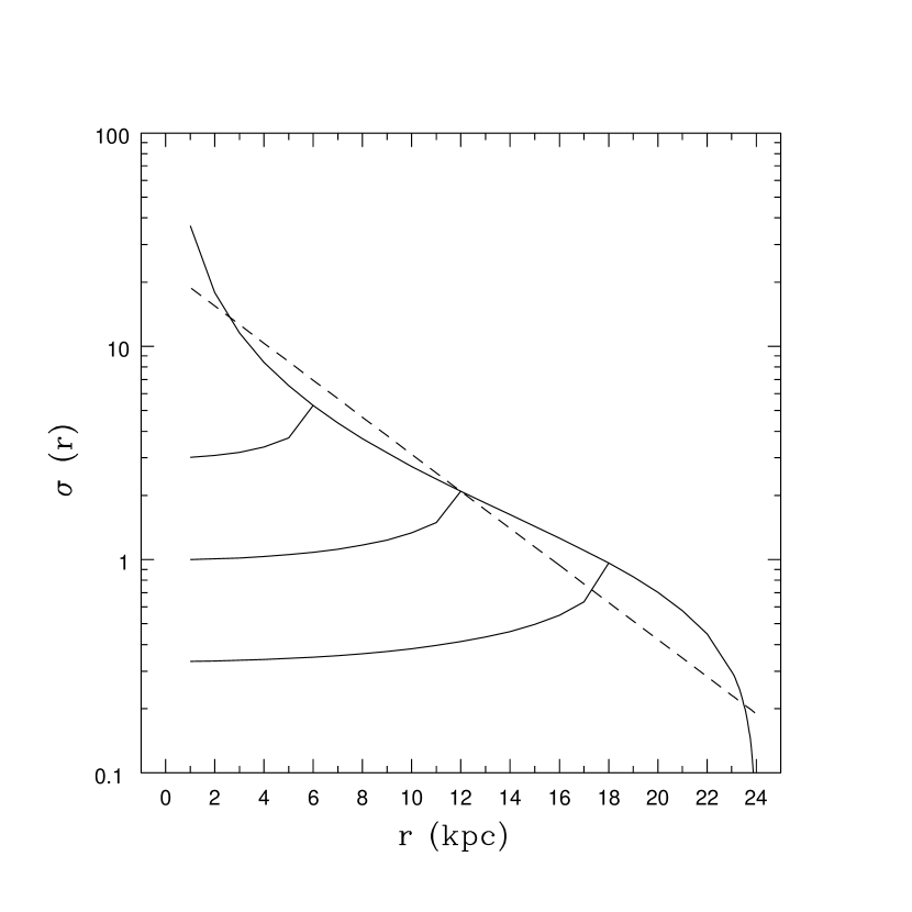
Figure 5 shows the surface density distributions resulting from this type of collapse, where the integral in equation (47) has been evaluated numerically. For the cases shown here, the initial radial extent of the pre-collapse gas was taken to be = , the rotation rate was chosen so that the centrifugal radius = 24 kpc (i.e., rad-1 for the Galactic parameters used previously), and all profiles have the same total mass. The four curves shown in Figure 5 correspond to varying values of the ratio = 2, 4, 8, and 16 (from top to bottom in the figure). For moderate values of the ratio , the surface density distributions have the same general form as those obtained previously (compare with Figs. 2 and 4).
This approach can be generalized to include any polytropic equation of state for the initially hydrostatic gas and any rotation profile . We start by writing the equation of state in the form
| (48) |
where is the polytropic index (e.g., Chandrasekhar 1939). The density distribution for hydrostatic equilibrium, in the limit where the dark matter halo dominates the gravitational potential, then takes the form
| (49) |
where the central density is specified through the relation
| (50) |
In the limit , the equation of state approaches an isothermal form; in the limit , , and the equation of state becomes adiabatic (for a monatomic gas). The polytropic index is thus confined to the range . We can see immediately that the value = 3 ( = 4/3) corresponds to a critical value: If , then the mass integral converges, whereas the mass integral diverges for .

Following the same formulation used above for the isothermal case, the disk surface density resulting from the collapse of a polytropic sphere with rotation profile takes the form
| (51) |
where = and = . As a consistency check, we can integrate this expression over the surface of the disk to find the total disk mass, and thereby obtain the expected result
| (52) |
For any polytropic index , the resulting surface density distributions display the same general form – with radial dependence somewhere between a truncated power-law and an exponential. In these disks, the outer radius is determined by the centrifugal barrier, which in turn is determined by the material with the highest specific angular momentum, and that material comes from the equatorial region at the outer boundary of the collapsing region. A collection of surface density profiles of this type is shown in Figure 6 for polytropic indices = 2 – 16. For the profiles shown here, the central density is assumed to be constant and the profiles are normalized to have constant total mass. For these parameter choices, the surface density profiles become steeper as the polytropic index increases. The resulting curves are close to straight lines on the plot of versus , where the effective scale radius of the exponential decreases with increasing polytropic index . Figure 6 also shows an exponential profile with scale length = 5 kpc (dashed curve). The surface density profile produced by the collapse of the = 8 polytrope has nearly the same slope. For comparison, models of galaxy groups and clusters have been used to estimate the equation of state in astrophysical systems (Ascasibar et al. 2003) and find a fit of the form , which corresponds to a polytropic index .
For completeness we note that for all polytropic indices , the total mass of the pre-collapse gaseous sphere is finite and disk solutions exist for the limit . In this case, the resulting surface density profiles approach power-law forms such that at large radii. However, the convergence to this power-law form is painfully slow.
3.6 Section summary
Actual galactic disks differ from the idealized disks found in this section in several ways. As outlined below, the single, spherical collapse picture must be generalized to allow for more complicated starting conditions (e.g., holes and filaments; see §4) and multiple disk accretion events (e.g., due to merging of subhalos, which supply additional gas; see §5). This work makes additional assumptions that can be studied in future work. We have not taken into account adiabatic contraction of the dark matter halo. This effect will make the gravitational potential well deeper and could be taken into account by changing the values of in the orbit solutions. A deeper potential well leads to greater infall velocities. Since the perpendicular component of the velocity is dissipated at the disk surface, the energy loss is greater for deeper potentials. For a given angular momentum, a deeper potential leads to a smaller centrifugal radius for a given orbit; notice, however, that the angular momentum of later orbits may be larger as well (e.g., Elmegreen et al. 2005) and lead to a larger centrifugal radius. This current treatment also makes the approximation of zero energy orbits and considers orbital solutions in the inner part of the potential. The latter approximation is not severe, since the orbits must be nearly radial in the outer part of the potential in order to reach the disk. Similarly, if the initial energy is small but nonzero, the orbit will be largely unchanged (where the basic constraint is ).
In addition, the calculation thus far determines the surface density profile resulting from the initial infall, i.e., the incoming gas parcels are assumed to stay at the radial locations where they fall. Over time, the disk will dissipate energy, transfer angular momentum, and spread out. Notice that a moderate amount of disk spreading (angular momentum transfer) will make the calculated surface density profiles look more like the exponential reference profile over the range of intermediate radii (roughly 2 – 20 kpc for the parameters used here). Notice also that real disk galaxies depart from an exponential law both on the inside and on the outside. The presence of galactic bulges causes the brightness profiles of observed disk galaxies to lie above that expected for an exponential disk at small radii, 1–2 kpc (see Binney & Merrifield 1998 for a detailed discussion of disk/bulge decomposition). On the outside, some disk galaxies show evidence for a cutoff radius that could be identified with in this theoretical treatment; typical values are kpc (van der Kruit & Searle 1981; Wainscot et al. 1988; Barteldrees & Dettmar 1994; Binney & Merrifield 1998).
4 GENERALIZED COLLAPSE SOLUTIONS
4.1 Partial radial coverage – shells and holes
This subsection considers configurations for which the initial (pre-collapse) gaseous sphere has holes, i.e., an evacuated central region. Suppose that the central portion of the sphere, with radius , has no gas. The corresponding surface density profile is that of the original sphere (with no central hole) with the contribution from a smaller sphere () removed. If the original sphere has radius and mass , and the hole region has radius and mass , the combined surface density profile is given by
| (53) |
where the surface density profiles on the right hand side of the equation are those obtained via the spherical collapse calculation of the previous section.
One example of collapse with a centrally evacuated region is shown in Figure 7. Here we consider the intermediate mass profile with = 2 () with constant rotation rate, and remove successively larger holes from the center of the starting state. The four curves shown in the figure correspond to the full sphere (top curve) and increasing fractions of the mass evacuated (25% to 75%). For comparison, the dashed curve shows an exponential surface density profile with the same mass as the surface density resulting from the collapse of the full sphere. As before, the rotation rate is chosen so that = 24 kpc.
4.2 Partial angular coverage
We can also use this formalism to determine the surface density profiles resulting from pre-collapse states with partial angular coverage. In general, the starting mass distribution can be restricted in both azimuthal angle and the polar angle . In this problem, the starting azimuthal angle determines the azimuthal angle where a given gas parcel will join the galactic disk, but it otherwise plays no role (e.g., starting angular momentum depends on but not ). Furthermore, after gaseous material has joined the disk, the differential rotation within the disk will eventually make the disk axisymmetric, thereby erasing any dependence on . Thus, if we consider starting states that are restricted in azimuthal angle (spheres with longitudinal slices removed), the net result is to reduce the total mass in the disk by a constant factor, but otherwise leave the surface density unchanged. We thus consider the case of restricting the starting state in polar angle .

Suppose we remove the polar cones from the starting state so that the polar angle is restricted to the range . The surface density contribution at a given radial location in the disk is the same as that produced by the collapse of the inner portion of the sphere with mass , where is given by the intersection of the ray and the locus of points for which material falls to radial position , i.e., the locus given by
| (54) |
Consider the case of an initial mass profile with = 2 () and constant rotation rate. If the starting state were a complete sphere it would have mass and outer (spherical) boundary . In this case, the polar cones are removed, where defines the opening angle of the cones. At a given radius in the disk, the surface density is the same as that for mass
| (55) |
The surface density profile is thus given by
| (56) |
where the upper limit of the integration is given by
| (57) |

Figure 9 shows the resulting surface density profiles for the intermediate starting mass profile with and constant rotation rate. The top curve shows the surface density profile for the complete sphere. The next three curves illustrate the effect of removing the polar cones from the starting configuration, where the opening angle is taken to be = , , and . For these three cases, the fraction of the total mass (within the same outer boundary) contained in the initial configuration, and hence the resulting disk, is = , , and , respectively.
4.3 The Limiting Case of Filaments
If we restrict the angular extent of a rotating sphere to its limiting form, the result is a filament, which provides a reference state for the (pre-collapse) initial conditions. Notice that a filament can be defined in a variety of ways. This treatment starts with a spherical initial condition, as considered above, and confines the geometry in both polar angle and azimuthal angle . In the limiting case, the resulting filament has all of its mass along a fixed ray defined by = constant and = constant. Further, this discussion is limited to cases where the rotation rate = constant, so that the filament has some angular momentum about the galactic center but it remains intact as it rotates. These filaments are thus highly idealized, but provide a useful benchmark for understanding the nature of galactic infall. Keep in mind, however, that these filaments are not the large scale structures (also called filaments) that connect galaxies to the cosmic web.
We begin by considering an isothermal initial configuration, so that , which will lead to a filament with constant mass per unit length. If we confine the starting sphere to a (narrow) range of polar angles , the resulting surface density can be written in the form
| (58) |
where and . Notice that we can confine the initial state in azimuthal angle to a narrow range without affecting result (up to the leading coefficient). In the limit that the range of polar angle is also small, , the integral in the above expression can be evaluated to obtain the result
| (59) |
where is the polar angle of the filament (so that and ; ). Next we want to write this expression for the surface density in terms of the effective mass per unit length of the filament. The mass contained within the boundary angles and is given by
| (60) |
In the limit of interest, where , the effective mass per unit length becomes
| (61) |
The surface density can be written in the form
| (62) |
For comparison, we also consider a filament with mass per unit length with a polar angle , where the mass in concentrated along a single ray (centered on the origin). Each point along the filament, given by its radial coordinate , has a particular angular momentum given by . As a result, conservation of mass implies that each point along the filament contributes to the surface density at a particular radius within the disk, i.e.,
| (63) |
Using the orbit solution from §2, we can relate the starting radial coordinate to the resulting disk radial coordinate , and find
| (64) |
where . Using the above expression to evaluate , the surface density (see equation [63]) can be written in the form
| (65) |
which is in agreement with the result of equation (62).
As in previous collapse solutions, we can define a centrifugal radius for filaments. For the case considered here with constant mass per unit length , this radius takes the form
| (66) |
where is the total mass that falls to the disk (from the filament). With this definition, the surface density becomes
| (67) |
The surface density thus takes a power-law form (here with index = 3/2) and has a sharp truncation radius at . Notice that if we integrate the surface density (eq. [67]) over the disk, we obtain the expected disk mass = (mass conservation is satisfied).
5 MULTIPLE COLLAPSE EVENTS
One defining characteristic of the current picture of dark matter halo formation is that mergers play an important role — small halos come together to forge larger bound structures. In most cases, some portion of the gas in the merging units eventually falls into the center of the composite structure, so that galactic disk formation must also involve a series of “accretion events”. The goal of this section is to incorporate these multiple accretion episodes into our description of gaseous disk formation (numerical simulations automatically include this process – see below). Here we assume that the gas contributed by each merging subhalo stacks up inside the gravitational potential of the larger composite structure; after cooling, the gas falls inward and thereby adds mass to the disk forming at the center. The galactic disk is thus assembled from inside-out, consistent with the standard scenario (e.g., Murali et al. 2002, Maller et al. 2006). Keep in mind that the assimilation of a smaller halo does not provide a fully formed disk, but rather provides a new source of gas for the composite disk. As a result, each accretion event produces a contribution to the surface density of the composite disk. Further, this contribution can be described as a disk surface density profile analogous to those calculated above. To summarize, this section develops a description of disk formation where a composite disk is assembled through the addition of many separately accreted disk layers, where each layer is provided by gas from a merging subhalo.222Although the net effect of merging halos is to add disk surface density profiles together, we stress that disks themselves are not merging. Instead, the merging halos provide a new gas supply for continued infall onto the disk. Notice also that we are making an assumption of timing, i.e., that incoming halos have not yet formed their disks.
Numerical simulations of hierarchical structure formation incorporate the idea of multiple accretion events in a natural way. The addition of mass into a developing halo is often described in terms of the halo mass assembly history (MAH), which has been well studied (e.g., Avila-Reese et al. 1998; Firmani & Avil-Reese 2000; Wechsler et al. 2002; van den Bosch 2002). This body of previous work indicates that the MAH is generally not dominated by major mergers; instead the MAH consists of a continuing series of smaller-scale events that can be described as a smooth aggregation of mass (Murali et al. 2002; Maller et al. 2006). In the (idealized) model developed herein, we consider each of these small-scale accretion events to provide a supply of gas that (after infall) results in a constituent surface density profile that contributes to the overall composite disk profile. The smooth nature of the MAH suggests that we must consider a large number of accretion episodes (each with a relatively small baryonic mass).
The distribution of angular momentum of the gas added during the accretion events determines the distribution of centrifugal radii for the constituent disks is thus an important quantity. We expect the newly added gas to have spin angular momentum inherited from the rotation of the subhalo that supplied the gas. In addition, the subhalo and its gas can have orbital angular momentum. Numerical simulations indicate that galactic spin parameters — and hence the spin angular momentum of subhalos and their gas — are drawn from a log-normal distribution (e.g., Bullock et al. 2001); these numerical studies also suggest that the width of the distribution . Although the angular momentum will include an additional orbital component, the latter cannot dominate; otherwise, the total angular momentum of the disks would be too large (see below). The distribution of orbital angular momentum is not known, but it will tend toward a log-normal distribution if a large number of physical variables play a role in setting the orbits (due to the central limit theorem; Richtmyer 1978). Another issue is that the angular momentum vectors (both spin and orbital) of the constituents are not necessarily aligned. Since the angular momenta add as vectors, this complication will act to make the total (composite) angular momentum smaller (than the result of adding scalars); further, this process adds another independent physical variable which (through the central limit theorem) will help simplify the composite distribution. As a result, we expect the distribution of total angular momentum to have nearly a log-normal form.
Before proceeding further, it is useful to summarize the ingredients of the calculation. The validity of this approach relies on the following assumptions: [1] The composite galactic disk forms as as superposition of gaseous layers, where each layer can be considered as a constituent disk with a power-law surface density distribution. We first consider equal mass constituents and then generalize to varying disk masses (which can be either correlated or uncorrelated with disk radius). [2] Each gaseous layer is assembled from the gas contributed by a subhalo that merges with the growing galactic halo. [3] During the merging process, the gas of each “accretion event” retains its component of angular momentum aligned with the overall sense of rotation of the galaxy. [4] During the course of a particular accretion event, infalling gas conserves its angular momentum and produces a surface density profile in accordance with the solutions of §2 – 4. The centrifugal radius of each disk layer is then determined by the total (spin and orbital) angular momentum of its progenitor subhalo. [5] Over the course of multiple merger events, the resulting distribution of (total) angular momentum is log-normal; as a result, the distribution of centrifugal radii is also log-normal with a well-defined peak value and width .
This calculation begins with the simplest case of equal mass constituent disks with the same general form, but with different centrifugal radii (which correspond to to different angular momenta of the pre-collapse gas). The basic problem is thus to add together an ensemble of contributing disk profiles with the form
| (68) |
where and is the centrifugal radius of the constituent disk (from the accretion or merger event). The function defines the shape of the edge, so that . The analysis given above shows that typical edge functions are and . The integer represents the number of events, and hence the total mass of the composite disk is specified by times a dimensionless factor given by the integral .
In our formalism, the above considerations imply that the ensemble of centrifugal radii are drawn from a log-normal distribution. Let be the radius at the peak of the distribution and let denote the width of the distribution. The composite disk surface density then takes the form
| (69) |
The sum can be evaluated by random sampling to determine the composite surface density profile of the disk. One example is shown in Figure 10, which uses the surface density distribution of equation (28) to specify the constituent profiles. The sum (69) is evaluated in the large limit. As expected, the composite surface density profile depends on the width of the log-normal distribution. For small values of the distribution width , all of the components are nearly the same and the composite profile looks much like that of the original constituents. In the limit of large width , the composite profile approaches a power-law form (, as derived below) over the range of radii of interest. In the realm of intermediate , the composite surface density profile is close to the exponential reference profile (shown by the dashed curve in Fig. 10). All of these results are robust (in that they are largely independent of the assumed constituent profiles) and can be understood analytically, as discussed below.

To study the problem of constructing composite surface density profiles, we need to evaluate the sum in equation (69). We consider the limiting case in which the disk edges are “sharp”, so that the edge function is a step function . For a given realization of the disk parameters, we then order the disk radii , from largest to smallest, and define to be the fraction of constituent disks with . The sum then becomes
| (70) |
Since the are log-normally distributed, we can convert the sum to an integral in the limit of large , where a large number of constituent disks are being assembled:
| (71) |
where = and is the natural logarithm of the centrifugal radii being integrated over. Recall that is a radial scale corresponding to the peak of the log-normal distribution and is the distribution width. Because the sum (eq. [70]) only includes disks with outer radii , the corresponding integral (eq. [71]) has a limited range of integration from out to . This integral can be written in terms of error integrals, which have a number of known properties (Abramowitz & Stegun 1972; hereafter AS72). In particular, we find
| (72) |
where . To approximate the integral, we make use of the well-known inequality,
| (73) |
which is valid for (AS72). This constraint allows us to write the composite surface density profile in the form
| (74) |
where both and are functions of the disk radial coordinate . The constant must lie in the range , and can be chosen to minimize the error. If we take = 3/2, the approximation to the integral in equation (73) is accurate to for all allowed values of the parameters, and is accurate to over the range of values needed to evaluate the surface density profile. Notice that this form is only valid for , which implies . For sufficiently large , however, this form is valid over most of the radial range of interest. These trends are illustrated in Figure 11, which shows the composite surface density calculated from random sampling compared to that obtained using the approximation of equation (74).

Now consider the composite distribution in the limiting cases. In the limit where the width of the distribution is narrow, the normal distribution (in the logarithm) becomes a Dirac delta function (see eq. [71]) and we recover the expected result
| (75) |
In the opposite limit of large width , equation (74) is valid for essentially all radii as long as , and we find that the composite surface density takes a power-law form, i.e.,
| (76) |
This resulting power-law form is independent of the index of the constituent disk profiles, as long as . Notice that the results of §3 show that for essentially all cases of physical interest, as indicated by equation (44). For large values of the initial index , all of the mass is concentrated toward the galactic center and the composite surface density profile always takes the form . This result follows from equation (72). As , becomes large and negative, the integral in equation (72) approaches a constant value (), and the composite surface density takes the form .
In the limiting case of , the disk edge becomes sharp, which (in a sense) is much steeper than an exponential falloff (at large ). In the opposite limit of large , the disk has a power-law form , which falls off more slowly than an exponential function. One might suspect that for some intermediate value of , the disk would obtain a roughly exponential shape, at least for some range of radii. This behavior does in fact occur, as shown in Figure 10, and can be understood in terms of the analytic approximation derived above. For radii sufficiently far from the origin so that equation (74) is valid, we can define an effective scale length for the surface density profile via
| (77) |
If this scale length were exactly constant, when considered as a function of , the surface density profile would be exponential. In practice, this function is slowly varying. Specifically, over the range of radii (which corresponds to ), the scale length varies by 10–12% for in the range 0.5 – 1.5, where the width is chosen to minimize the variation. This optimization requires values of = 0.3 – 0.5, which are comparable to, but somewhat smaller than, the widths of the distributions deduced from numerical simulations (where ; Bullock et al. 2001).
The discussion thus far assumes that each constituent disk has a constant mass (equal to ). However, the formalism is sufficiently robust to consider the general case of varying disk masses. The composite profile will not change as long as the disk masses are uncorrelated with the centrifugal radius of the individual components. Specifically, suppose that the mass of each component disk has the form
| (78) |
where is a random variable with unit mean. The masses are uncorrelated when = 0 and show a correlation with the centrifugal radius for . If we propagate this ansatz through the formalism given above, the composite disk profile takes the form
| (79) |
where the variable . Notice that the effect of the random variable is completely washed out in the limit of a large number of accretion events. In the limit of a narrow distribution, we again recover the expected result that the composite distribution is the same as that of the components (eq. [75]). In the limit of a wide distribution, the composite surface density profile becomes a power-law with index , independent of the index of the component profiles, as long as . For “large” values of , the composite surface density takes the form of the original profiles so that .

The results presented thus far have been calculated in the limit of large , so that the surface density of the composite system approaches a particular smooth form. An interesting question is to ask how large must be in order for the problem to be safely in the large limit. One way to answer this question is to calculate the RMS deviation of the difference between the composite surface density obtained with a “small” value of and that of the large limit. Notice, however, that for small , each realization of the random values (the ) will lead to a somewhat different profile and hence a different measure of the RMS error. Roughly speaking, for = 10, we get deviations of about 50 percent, for = 100 the deviations are about 10 percent, and for = 1000 the deviations are only about 2 percent. These deviations are computed over the range ; they are greater at larger radii. Another way to address this issue is to plot the resulting surface density profiles for varying numbers of the constituent disks. The result is shown in Figure 12 for logarithmically spaced = 1, 4, 16, 64, and 256. As the number of constituent disks increases, the profiles approach that of the asymptotic (large ) limit shown by the heavy solid curve in Figure 12. Keep in mind that the profiles will vary greatly from realization to realization for small values of ; in other words, the small- profiles shown in the figure will look different every time they are computed (with independent sampling). Nonetheless, for , the composite surface density has roughly the same form as that of the asymptotic limit out to . Similarly, for , the surface density profile will be similar to the asymptotic limit out to . This result is important, since galaxy sized halos are thought to be assembled from moderate numbers of component halos (Wechsler et al. 2002).
This formalism can be applied to any scenario in which the net effect is to add surface density profiles together. As one example, it can account for cosmological evolution of the background potential. In the approximation used here, the surface density profiles of the constituent disks add together so that the final state does not depend on the order in which they are assembled. In a cosmological setting, however, dark matter halos become steadily larger, both from continued infall from large distances and through the mergers of smaller halos. As a result, the depth of the gravitational potential well () increases with time. If the constituent disks result from the collapse of gas that attains hydrostatic equilibrium (§3.5), then the pre-collapse extent of the gas will be smaller at later times (for a fixed mass), and the corresponding centrifugal radius will be a decreasing function of time if angular momentum is constant. On the other hand, some observations (Elmegreen et al. 2005) and theoretical work (Firmani & Avila-Reese 2000) indicate that disk radii should increase with time. This result can be made consistent with our multiple accretion scenario if the specific angular momentum increases for subsequent accretion events. In any case, the time dependence of the centrifugal radii can be taken into account in the distribution of . If the distribution is log-normal, as assumed here, then the final result depends only on the peak value and width of the distribution. However, this procedure can be generalized to other distributions. As another example, some numerical simulations suggest that baryons can transfer angular momentum to the dark matter so that gas falling in later would have a systematic shift in its angular momentum distribution (private communication, anonymous referee); the effect of this process on the resulting surface density profile of the disk could be studied with the formulation developed here.
This analysis shows that a composite disk can display a nearly exponential surface density profile, provided that the distribution of centrifugal radii has an intermediate width () and the constituent disks have power-law indices . Both of these conditions are expected to be met, as outlined above. Notice that when an exponential surface density profile is realized, the scale length is roughly (Figs. 10, 11, 12), where is the centrifugal radius at the peak of the distribution. To produce scales kpc, as indicated by observations (Binney & Merrifield 1998), the radius must lie in the range = 11 – 14 kpc. The centrifugal radius of an individual constituent disk depends on the spin parameter through a relation of the form , where is a dimensionless parameter of order unity. For example, if the halo has a Hernquist profile, the gas density follows that of the dark matter, and all of the gas out to falls in, then . With typical halo scale radii = 50 – 70 kpc and spin parameters = 0.035 – 0.04 (at the peak of the distribution – see Bullock et al. 2001 and Wechsler et al. 2002), the expected peak value of the centrifugal radius would lie in the range = 7 – 11 kpc. These values of are thus comparable to, but somewhat lower than, those required to produce the correct disk scale length. However, the values quoted above only include the spin angular momentum of the constituent gas modules. As these subunits fall into the larger halo and merge, and thereby add their gas to the growing structure, they contain orbital angular momentum in addition to that described by the spin parameter . If the orbital angular momentum is roughly comparable to (but smaller than) the spin angular momentum, the constituent disks will have the proper total angular momentum for this multiple infall process to produce exponential composite disks with the observed scale length.
6 CONCLUSION
6.1 Summary of results
This paper has studied the assembly of galactic gaseous disks by following orbit solutions for baryonic gas parcels as they fall through the potential wells of dark matter halos. Our general analytic formulation of the problem (as presented in §2) is robust and can be used in variety of contexts. In this paper, we calculate the velocity fields of the incoming gas, the density distribution of the gaseous material as it falls inward, and the surface density profiles of the resulting gaseous disks. Our specific results are summarized below:
[1] The generic outcome for a gaseous disk produced by a single spherical collapse is a power-law surface density that is truncated at a centrifugal radius (see Figs. 2, 4, and 5). Here, the centrifugal radius is the radius to where the material with the highest (initial) specific angular momentum falls during the collapse. This result suggests that the “fundamental units” of galactic disk assembly are not exponential disks, but instead are truncated power-laws. For a constant rotation rate of the initial gaseous sphere, the power-law index of the surface density distribution () depends on the initial mass distribution such that , where is the power-law index of the starting mass profile (). For a rotation rate that varies with radius according to , the power-law index of the resulting disk surface density is given by . We also determined the density profiles appropriate for hydrostatic equilibrium of both isothermal and polytropic gas in the background potential of a dark matter halo (§3.5) and followed the subsequent collapse (Figs. 5 and 6). For polytropic equations of state with relatively large indices , the resulting surface density profiles are close to exponential (except near the centrifugal barrier).
[2] In addition to determining the disk surface density profiles, this calculation provides an analytic description of the dynamics that builds up galactic disks. This description includes the velocity fields of the gas during the collapse (eq. [8]), the density distribution of the infalling baryonic material (eqs. [10] and [16]), and the mapping between the starting locations in the pre-collapse cloud and the “final” radial positions within the disk (e.g., Figs. 3 and 8). We also obtain analytic forms for the hydrostatic equilibrium profiles of polytropic gaseous spheres in the gravitational potential of a dark matter halo (eqs. [45] and [49]).
[3] This collapse picture has been generalized to include less idealized starting configurations (§4). The first generalization considers the starting gaseous spheres to have evacuated regions in their centers. The signature of these central holes in the starting states is to produce impoverished central regions in the corresponding gaseous disks (see Fig. 7). The starting states can also be considered to have limited angular extent. The removal of the polar caps from the initial states also leads to a deficit of material in the disk centers (relative to the spherical initial state) as shown in Figure 9.
[4] This formulation of the collapse problem can be further generalized to include multiple accretion events, which are expected to occur due to merging of individual halos to form larger, composite structures (§5). Each incoming halo provides a new supply of gas, which subsequently cools and falls inward to produce another component to the disk. Here we consider the addition of a large number of such constituent disks, where the centrifugal radii are drawn from a log-normal distribution (consistent with the numerical finding that halo spin parameters display a log-normal distribution) and find an interesting and somewhat unexpected result: The addition of a large number of power-law disk profiles with index results in a composite surface density profile of the form in the limit of a wide distribution for , where this result is independent of the index (provided that ). In the limit of a narrow distribution of , the composite surface density is the same as the constituent surface density profiles. In the intermediate regime, however, the composite surface density can display a nearly exponential form over a range of radii (Figs. 10 and 11). The asymptotic forms are obtained in the limit of large numbers of constituent disks, and the approach to large is shown in Figure 12. Although the large limit is approached rather slowly, this sequence shows that tens of subunits (constituent disks) are necessary to produce a smooth disk with a nearly exponential surface density profile.
6.2 The quest for exponential disks
One of the defining features of observed disk galaxies is that their surface brightness distributions display a nearly exponential form. One might hope that numerical simulations of galaxy formation would naturally produce gaseous disks with exponential surface density profiles, so that star formation could take place in situ and thereby account for the observations. Unfortunately, the production of exponential surface density profiles is not automatic. Building upon earlier work (Dalcanton et al. 1997, van den Bosch 2001, Kaufmann et al. 2006, and many others), this paper shows that the fundamental disks produced by a single collapse event have the form of a truncated power-law rather than an exponential profile (Figs. 2 and 4). The transformation between these truncated power-law forms and exponential profiles most likely involves several processes, as outlined below:
[A] The observed disk brightness profiles are close to exponential only over a limited range of radii (roughly 2 – 20 kpc) and a correspondingly small range of scale lengths (roughly ). The inner regions depart from an exponential form due to contamination from bulge components and the outer regions are too faint to be observed. Further, as shown by Figure 2, the difference between a truncated power-law and an exponential is not too large over a limited range of radii. One of the largest differences between the power-law profiles and an exponential profile occurs at small radii, where the power-law profiles have cusps; this discrepancy is largely alleviated, or at least masked, by the presence of the bulge component (for kpc). In addition, if the initial (pre-collapse) gas departs from a complete spherical form, either through inner evacuated regions or the removal of polar caps, then the resulting surface density profiles will not have inner cusps (Figs. 7 and 9), or they will be less pronounced.
[B] The calculation presented in this paper accounts for only the formation of the disk, not its subsequent evolution. If galactic disks are produced with sharp edges (as indicated here for the case of a single collapse event), then gravitational instabilities will grow robustly and cause the disk to spread. Although previous authors (Dalcanton et al. 1997) have argued that the time scale for such instability is too long, the quoted (long) time scales are appropriate for disks that already have soft (e.g., exponential) edges. If disks have sufficiently hard edges, as produced here, then gravitational instabilities can grow on the dynamical time scale of the outer disk edge (Adams et al. 1989; Ostriker et al. 1992). This time scale is given by the inverse of the orbital frequency at the centrifugal radius, roughly 100 Myr (/20 kpc). This time scale is still somewhat long to account for all of the necessary angular momentum redistribution, but gravitational instabilities will have time to grow and act to spread out the disk. Notice that a truncated power-law profile that spreads out will become more like an exponential profile.
[C] Exponential profiles are observed for the surface brightness distributions of galactic disks, not the surface density of the gas, so it is possible for the star formation process to help produce the observed exponential forms. A good demonstration of this effect is found in Lin & Pringle (1987), where initial surface density profiles roughly like those of Figure 2 spread out under the action of disk viscosity and convert some fraction of the mass into stars. The resulting surface density of the stars is much more like an exponential form than the starting gas profile.
[D] Finally, as shown in §5, the addition of multiple disk surface density profiles can produce a composite profile that displays a nearly exponential form — much more like an exponential than the initial (constituent) starting profiles. The ingredients necessary to produce a nearly exponential profile are a large number of constituent disks and a log-normal distribution for their centrifugal radii. This result is independent of the shape of the constituent disk profiles as long as they have effective power-law indices . Since the current paradigm of structure formation indicates that galaxies are assembled through a process of hierarchical merging, multiple accretion events are highly likely. Further, numerical simulations suggest that the distribution of halo angular momentum is log-normal (Bullock et al. 2001) so that the distribution of centrifugal radii is also expected to be log-normal.
In practice, all four of these considerations (and perhaps others) will conspire to produce the observed exponential disk profiles. Individual infall events will each produce disk surface density profiles that are truncated power-laws, but multiple infall events will jointly build up a nearly exponential disk (as shown in Fig. 10). The effects of star formation, viscous spreading, and disk evolution via gravitational torques will act to smooth out the disk and drive the surface density towards a more exponential form. Given the presence of the bulge contribution at small radii and the limited dynamic range of the observed profiles, the exponential disks in observed galaxies can be understood through the joint action of these processes.
Acknowledgment
We would like to thank Michael Busha, Gus Evrard, and Lars Hernquist for many beneficial discussions. This work was supported at the University of Michigan by the Michigan Center for Theoretical Physics; by NASA through the Terrestrial Planet Finder Mission (NNG04G190G) and the Astrophysics Theory Program (NNG04GK56G0); and by NSF through grants DMS01038545 and DMS0305837. Finally, we thank the referee for a comprehensive and detailed set of comments that improved the manuscript.
References
- (1) Abramowitz, M., & Stegun, I. A. 1972, Handbook of Mathematical Functions (New York: Dover), (AS72)
- (2) Adams, F. C., & Bloch, A. M. 2005, ApJ, 629, 204 (AB05)
- (3) Adams, F. C., Ruden, S. P., & Shu, F. H. 1989, ApJ, 347, 959
- (4) Ascasibar, Y., Yepes, G., Müller, V., & Gottlöber, S. 2003, MNRAS, 346, 731
- (5) Avila-Reese, V., Firmani, C. & Hernández, X. 1998, ApJ, 505, 37
- (6) Barteldrees, A., & Dettmar. R.-J. 1994, A&AS, 103, 475
- bm (98) Binney, J., & Merrifield, M. 1998, Galactic Astronomy (Princeton: Princeton Univ. Press)
- bt (87) Binney, J., & Tremaine, S. 1987, Galactic Dynamics (Princeton: Princeton Univ. Press)
- (9) Bullock, J. S., et al. 2001, ApJ, 555, 240
- (10) Busha, M. T., Evrard, A. E., Adams, F. C., & Wechsler, R. H. MNRAS, 363, L11
- Cassen & Moosman (1981) Cassen, P., & Moosman, A. 1981, Icarus, 48, 353
- (12) Chandrasekhar, S. 1939, Stellar Structure (New York: Dover)
- Chevalier (1983) Chevalier, R. 1983, ApJ, 268, 753
- (14) Dalcanton, J. J., Spergel, D. N., & Summers, F. J. 1997, ApJ, 482, 659
- (15) Elmegreen, B. G., Elmegreen, D. M., Vollbach, D. R., Foster, E. R., & Ferguson, T. E. 2005, ApJ, 634, 101
- (16) Evrard, A. E., Summers, F. J., & Davis, M. 1994, ApJ, 422, 11
- (17) Fabian, A. C., Nulsen, P.E.J., & Canizares, C. R. 1984, Nature, 310, 733
- (18) Fall, S. M., & Efstathiou, G. 1980, MNRAS, 193, 189
- (19) Firmani, C., & Avila-Reese, V. 2000, MNRAS, 315, 457
- (20) Gebhardt, K. et al. 2000, ApJ, 539, L13
- (21) Governato, F., Mayer, L., Wadsley, J., Gardner, J. P., Willman, B., Hayashi, E., Quinn, T., Stadel, J., & Lake, G. 2004, ApJ, 607, 688
- (22) Gunn, J. 1982, in Astrophysical Cosmology, eds. Bruck, Coyne & Longair (Vatican: Pontificia Academia Scientiarum), p. 233
- (23) Hernquist, L. 1990, ApJ, 356, 359
- k (96) Kauffmann, G. 1996, MNRAS, 281, 475
- (25) Kaufmann, T., Mayer, L., Wadsley, J., Stadel, J., & Moore, B. 2006, MNRAS, in press, astro-ph/0601115
- (26) Keres, D., Katz, N., Weinberg, D. H., & Davé, R. 2005, MNRAS, 363, 2
- (27) Lin, D.N.C., & Pringle, J. E. 1987, ApJ, 320, L87
- (28) Maller, A. H., Katz, N., Kereš, D., Davé, R., & Weinberg, D. H. 2006, ApJ, 647, 763
- (29) Murali, C., Katz, N., Hernquist, L., Weinberg, D. H., & Davé, R. 2002, ApJ, 571, 1
- (30) Navarro, J. F., Frenk, C. S., & White, S.D.M. 1997, ApJ, 490, 493 (NFW)
- (31) Ostriker, E. C., Shu, F. H., & Adams, F. C. 1992, ApJ, 399, 192
- (32) Rees, M. J., & Ostriker, J. P. 1977, MNRAS, 179, 541
- (33) Richtmyer, R. D. 1978, Principles of Advanced Mathematical Physics (New York: Springer-Verlag)
- (34) Robertson, B., Yoshida, N., Springel, V., & Hernquist, L. 2004, ApJ, 606, 32
- (35) Shu, F. H. 1990, Gas Dynamics: The physics of astrophysics II (Mill Valley: Univ. Science Books)
- (36) Spergel, D. N. et al. 2003, ApJS, 148, 175
- Terebey, Shu, & Cassen (1984) Terebey, S., Shu, F. H., & Cassen, P. 1984, ApJ, 286, 529
- (38) Thacker, R. J., & Couchman, H.M.P. 2001, ApJ, 555, L17
- (39) Ulrich, R. K. 1976, ApJ, 210, 377
- vdb (01) van den Bosch, F. C. 2001, MNRAS, 327, 1334
- vdb (02) van den Bosch, F. C. 2002, MNRAS, 331, 98
- (42) van der Kruit, P. C., & Searle, L. 1981, A&A, 96, 116
- (43) Wainscot, R. J., Freeman, K. C., & Hyland, A. R. 1988, ApJ, 337, 163
- (44) Wechsler, R. H., Bullock, J. S., Primack, J. R., Kravtsov, A. V., & Dekel, A. 2002, ApJ, 568, 52
- (45) White, S.D.M., & Frenk, C. S. 1991, ApJ, 379, 52
- (46) White, S.D.M., & Rees, M. J. 1978, MNRAS, 183, 341