Light Curves for Rapidly-Rotating Neutron Stars

Abstract

We present raytracing computations for light emitted from the surface of a rapidly-rotating neutron star in order to construct light curves for X-ray pulsars and bursters. These calculations are for realistic models of rapidly-rotating neutron stars which take into account both the correct exterior metric and the oblate shape of the star. We find that the most important effect arising from rotation comes from the oblate shape of the rotating star. We find that approximating a rotating neutron star as a sphere introduces serious errors in fitted values of the star’s radius and mass if the rotation rate is very large. However, in most cases acceptable fits to the ratio $M/R$ can be obtained with the spherical approximation.

1. Introduction

One of the most fundamental problems in neutron star astrophysics is the determination of the mass-radius relation through observations. This would allow the observational determination of the equation of state (EOS) of cold supernuclear density material. While the measurement of mass is possible if the star is in a binary, neutron stars are too small to allow a direct measurement of their radii. One promising indirect method for inferring the radius is through observations and modeling of light curves for X-rays emitted from X-ray pulsars and neutron stars that exhibit type I X-ray bursts. This method requires the raytracing of photons emitted from the star’s surface in order to predict the signal detected by the observer. In this paper we present the first raytracing calculations for rapidly-rotating neutron stars that include the correct metric and correct shapes of the star, as well as allowing for arbitrary emission and detection directions.

Rapidly-rotating neutron stars are a promising target for an effort to constrain the EOS since observations of their light curves could potentially allow the determination of a star’s mass and radius. In the case of a slowly rotating neutron star, the light curve characteristics are controlled by the ratio $M/R$, but the value of $M$ or $R$ for the star is not observable through the light curve. However, if the star is rapidly-rotating, the Doppler boost resulting when the star’s equatorial velocity is of the order $v/c\sim 0.1$ or larger creates an asymmetry in the light curve which makes it possible to measure $v$. Since the spin frequency is always known, the star’s radius can be extracted. Knowledge of $R$ and $M/R$ could then potentially be used to constrain the EOS. The purpose of this paper is to determine how accurately these two parameters can be determined through light curve fitting.

In this paper we investigate the effect of rapid rotation on pulse shapes. In order to isolate these effects, we have chosen to simplify our treatment of the shape, size, location and emissivity of the emitting region. It should be understood that the effects due to rapid rotation discussed in this paper are only one ingredient in the modeling of pulse shapes and it will be necessary to combine these effects with more realistic treatments of the emitting regions in order to model real data.

In order to proceed with a program of fitting light curves in order to infer the radius of a neutron star a number of assumptions must be made. The most fundamental assumption made in this paper is that the light originates from the surface of the star and that no material lying between the star and observer causes scattering. We make this assumption so that we can focus on the effects due to rotation on the pulse shape, but it is possible that light is emitted from an extended region off of the star’s surface and that the light interacts with the matter surrounding the star. For example, in the case of the slowly rotating X-ray pulsars complicated accretion columns are needed in order to fit the observations (Leahy, 2004). Pulse shape models of real data should allow for the possibility of extended emission regions.

Another important input to light curve models is the spectrum and emissivity of the emitting region. In the case of the 2.5 ms X-ray pulsar SAX J1808.4-3658, Poutanen & Gierliński (2003) have shown that a hybrid spectrum including blackbody and Comptonized emission is needed. In their models, thermal emission is directed towards the normal to the surface and the Comptonized emission is directed away from the normal, creating a strong anisotropy. Other models for the pulse shapes observed in type I X-ray bursts suggest anisotropic emission as well (Miller & Lamb (1998), Bhattacharyya et al. (2005)). Any anisotropy in the emission is known to have a strong effect on the light curve, so realistic light curve models must include the effects of anisotropy. In our present work, we have simplified our models to only allow isotropic emission. We expect that the magnitude of the rotational effects discussed in this paper are similar to the magnitude of the effects caused by anisotropic emission.

The assumed shape of the emitting region also strongly affects the pulse profile. Most studies have focused on either infinitesimal spots or simple Gaussian profiles. Recently Kulkarni & Romanova (2005) have produced MHD simulations of accretion flows onto neutron stars that show the hot spots on X-ray pulsars could have more complicated shapes, confirming predictions made by Ghosh & Lamb (1978). For the case of type I X-ray bursts it is possible for normal modes to be excited (Heyl, 2004), which would produce patterns associated with the modes (Heyl, 2005; Lee & Strohmayer, 2005). In our calculations we have chosen the simplest possible pattern (an infinitesimal uniform brightness spot) in order to focus on the effects due to rotation. Models of real data must allow for more complicated emission shapes and brightness patterns.

The gravitational field outside of the star is important, for it gravitationally redshifts the photons and bends their direction of propagation. For non-rotating stars the Schwarzschild metric is all that is required to describe the photon trajectories (Pechenick, Ftaclas, & Cohen, 1983). The Schwarzschild + Doppler (S+D) approximation (Miller & Lamb, 1998; Poutanen & Gierliński, 2003) was introduced as a simple method for calculating the light curves of slowly rotating stars. In the S+D approximation the gravitational field is modeled by the static Schwarzschild solution and the rotational effects are approximated by using the special relativistic Doppler transformations. One of the goals of this paper is to find the conditions under which the S+D approximation will fail. For rapidly-rotating neutron stars, the metric must be computed numerically using one of many known algorithms, such as that of Cook, Shapiro, & Teukolsky (1994). The Kerr black hole metric can be made to agree to first order in angular velocity with the metric of a rotating neutron star metric by choosing the Kerr parameter $a$ to be $J/M$ where $J$ is neutron star’s angular momentum. The Kerr black hole is a poor approximation to a rotating neutron star for spin frequencies above 400 Hz (for an example involving the innermost stable circular orbit, see Miller et al 1998). However, some calculations (Braje et al 2000) have suggested that the Kerr metric may suffice for raytracing applications. This motivates (Braje, Romani, & Rauch, 2000; Bhattacharyya et al., 2005) the use of the Spherical Kerr approximation (SK) where a spherical surface is embedded in the Kerr spacetime. In this paper we will show that when the S+D approximation fails, the SK approximation also fails, so that the SK approximation is not necessarily a better choice than S+D. In this paper we compute the metric of rapidly-rotating neutron stars using realistic equations of state and perform raytracing on the computed numerical spacetime. In a previous paper (Cadeau, Leahy, & Morsink, 2005) (CLM) we performed similar calculations that were restricted to the equatorial plane. In this paper we generalize to allow arbitrary initial spot locations and arbitrary observer locations.

The final important input to a raytracing program is the shape of the star’s surface, which for a rotating fluid star is an oblate spheroid. In almost all previous calculations it has been assumed that the surface of the star is a sphere, irrespective if the exterior gravitational field was assumed to be Schwarzschild or Kerr. We are aware of only one previous calculation, by Braje & Romani (2001) that takes the oblate surface into account. In that paper they consider further scatterings of photons within the magnetosphere, so that the effect of oblateness is not clearly separated from other effects. In order to motivate the choice of a spherical surface, it is often stated that the ratio of polar axis to equatorial axis is very close to unity, even for rapid rotation. However, this ratio is neither coordinate invariant, nor directly observable. The oblate shape of the star has two main effects. (I) The gravitational field near the the poles is stronger than near the equator, so the redshift and photon deflection are larger for photons emitted near the poles. (II) Light is emitted at different angles with respect to the normal to the surface if the surface is an oblate spheroid instead of a sphere. As a result some parts of a spherical star that an observer can’t see will be visible if the star is actually oblate (the converse is also true). Of these effects, the second is the most important, and leads to failure of the S+D and SK approximations for rapid rotation.

Another application which makes use of raytracing is the calculation of absorption line profiles. Absorption line profiles have been computed in the past using the S+D approximation (Özel & Psaltis, 2003; Villarreal & Strohmayer, 2004) and using the SK approximation (Bhattacharyya, Miller & Lamb, 2006). Interestingly, Bhattacharyya, Miller & Lamb (2006) have identified signs of frame-dragging in the line profiles computed using the Kerr metric for very rapidly-rotating neutron stars. Chang et al. (2006) compared line profiles using oblate stars (using the same type of method used in this paper) with the line profiles calculated in the spherical approximation and found that the differences are insignificant for line profile calculations. However, it should be noted that the calculations done by Chang et al. (2006) assumed that light from all of the star contributes to the line profile, which would tend to average out differences arising from the shape of the star.

In this paper we wish to explore the rapid rotation effects of the metric and oblateness on the calculated light curves of neutron stars and on the fitting of a star’s mass and radius from the light curves. In order to isolate these effects, we consider the simplest possible assumptions for all other aspects. We assume isotropic emission from an infinitesimal spot, but allow for spots and observers at any location. As discussed in the previous paragraphs, there is enormous uncertainty in the shape, size and emissivity of the emitting regions which will have the effect of making it difficult to discern the relativistic effects discussed in this paper. However, we will show that for very rapidly rotating neutron stars, the relativistic rotational effects are large and should be incorporated in models of real data. In section 2 we describe the method used to compute the light curves for rotating neutron stars. In section 2.8 we outline the four types of approximation schemes that could be used to produce light curves. In section 3 we compare the light curves from the exact and approximate methods. We show how programs that attempt to fit light curves using either spherical approximation will converge to incorrect values of mass and radius at spin frequencies larger than about 300 Hz, although they may converge to the correct value of the ratio $M/R$. We conclude with a discussion of these results in section 4.

2. Light Curve Calculations for Rapid Rotation

The metric of a rotating neutron star can be accurately computed using a public-domain code rns (Stergioulas & Friedman, 1995) based on the code by Cook, Shapiro, & Teukolsky (1994). This code computes the four metric potentials $\alpha,\gamma,\rho$ and $\omega$, that appear in the general stationary axisymmetric metric

$$ds^{2}=-e^{\gamma+\rho}dt^{2}+e^{2\alpha}\left(d{\bar{r}}^{2}+{\bar{r}}^{2}d\theta^{2}\right)+e^{\gamma-\rho}{\bar{r}}^{2}\sin^{2}\theta(d\phi-\omega dt)^{2},$$ (1)

where the metric potentials are functions of only ${\bar{r}}$ and $\theta$. The interpretation of these potentials and coordinates has been discussed in more detail in CLM.

We have chosen two equations of state (EOS) from the Arnett & Bowers (1977) catalog which span a realistic range of stiffness (although we have not included quark stars). EOS A is one of the softest EOS and EOS L is one of the stiffest. While these EOS are rather old-fashioned and the physical assumptions made in deriving these EOS are now considered too simplistic, these EOS do provide a wide span of properties that allow us to illustrate the different levels that rotation can affect the resulting light curves. Modern EOS, such as EOS APR (Akmal et al. (1998)) have properties that are bracketed by the older EOS A and L.

We have restricted our computations to stars with masses of $1.4M_{\odot}$ and spin frequencies from 100 to 600 Hz in 100 Hz increments in order to explore the spin dependent effects. The 1.4 $M_{\odot}$ stars constructed from EOS A have equatorial radii ranging from 9.5 to 9.8 km (depending on the spin rate) allowing for compact stars. The 1.4 $M_{\odot}$ stars constructed with EOS L have equatorial radii ranging from 14.8 to 16.4 km allowing for larger stars that are strongly affected by rotation. In contrast to the extreme EOS used in our calculations, a $1.4M_{\odot}$ neutron star constructed from the modern EOS APR has an equatorial radius ranging from 11.4 to 11.8 km as the spin is increased from 0 Hz to 600 Hz. The properties of the neutron star models used in this paper are summarized in Table 1. In Table 1 we show the values of the compactness $M/R$ and the speed of the star $v$ at the equator. The stars constructed with EOS A are more compact than the EOS L stars, so the effects of light-bending and time-delays are most important in the EOS A stars. The equatorial velocities are highest for the the larger EOS L stars. As an alternative to the equatorial velocity of the star, the dimensionless rotation parameter $j=J/M^{2}$ (where $J$ is the star’s angular momentum) is a useful measure of the importance of rotation for the star. The effect of oblateness is quadratic in the parameter $j$, so the EOS L stars with high spin frequencies are very oblate while the more compact stars are only slightly oblate. In addition, if the neutron star has a mass larger than $1.4M_{\odot}$ then it will be more compact and less affected by rotation.

The fastest neutron stars in X-ray binaries have spin frequencies near 600 Hz, motivating our range of spin frequencies. The recent discovery (Hessels et al., 2006) of a 716 Hz binary radio pulsar suggests that 700 Hz X-ray pulsars may be discovered in the future, but for the present purposes, stars spinning at 600 Hz serve to illustrate the largest effects due to rotation.

2.1. Geodesic Equations

The geodesic equations for the coordinate positions of a photon depend on the impact parameter $b$ defined by the ratio of the photon’s angular momentum to its energy. The equations are integrated with respect to an affine parameter $\lambda$ scaled so that photon propagation is independent of the photon’s energy. We use an overdot to denote differentiation with respect to $\lambda$. The form of the geodesic equations used in our integration is

$$\dot{t} = e^{-(\gamma+\rho)}(1-\omega b)$$ (2)

$$\dot{\phi} = \omega e^{-(\gamma+\rho)}(1-\omega b)+e^{\rho-\gamma}\frac{b}{\bar{r}^{2}\sin^{2}\theta}$$ (3)

$$\ddot{\bar{r}} = -\alpha_{,\bar{r}}\left(\dot{\bar{r}}^{2}-\bar{r}^{2}\dot{\theta}^{2}\right)-2\alpha_{,\theta}\dot{\bar{r}}\dot{\theta}+\bar{r}\dot{\theta}^{2}+\frac{1}{2}e^{-2\alpha}\mathcal{B}_{,\bar{r}}$$ (4)

$$\ddot{\theta} = \alpha_{,\theta}\left(\frac{\dot{\bar{r}}^{2}}{\bar{r}^{2}}-\dot{\theta}^{2}\right)-2\left(\alpha_{,\bar{r}}+\frac{1}{\bar{r}}\right)\dot{\bar{r}}\dot{\theta}+\frac{1}{2\bar{r}^{2}}e^{-2\alpha}\mathcal{B}_{,\theta}$$ (5)

$$\mathcal{B} = e^{-(\gamma+\rho)}(1-\omega b)^{2}-\frac{b^{2}e^{\rho-\gamma}}{\bar{r}^{2}\sin^{2}\theta}.$$ (6)

These equations are overspecified, since the fact that photon’s four-velocity vector has vanishing norm leads to the momentum constraint

$$\dot{\bar{r}}^{2}+{\bar{r}^{2}}\dot{\theta}^{2} = e^{-2\alpha}{\mathcal{B}}(\bar{r},\theta)\equiv{\mathcal{A}}(\bar{r},\theta)$$ (7)

which provides an extra relation between $\dot{\bar{r}}$ and $\dot{\theta}$, and defines the function $\mathcal{A}=e^{-2\alpha}\mathcal{B}$. While it would be possible to eliminate equation (5) using equation (7), this would not allow us to evaluate the accuracy of the code. We have chosen to integrate equations (2) - (5) and use the momentum constraint equation as a test of the code’s accuracy. Our code uses a Runge-Kutta algorithm with adaptive step size.

The main addition to the existing rns code which we made was a calculation of the derivatives of the metric potentials which are required for the geodesic integration. A simple finite differencing scheme will fail at the poles of the star and also tends to unacceptably large errors far from the star. Instead, we take advantage of the explicit sum formulae (Komatsu, Eriguchi & Hachisu, 1989) for the potentials and explicitly take their first derivatives with respect to $\bar{r}$ and $\theta$ as well as the mixed second derivative. This provides a smooth set of potentials and derivatives at discrete grid points which can be used in a bicubic interpolation scheme (Press et al., 1992) to find the values of the potentials and their derivatives at intermediate points.

2.2. Initial Conditions

The surface of the star is described by the function $\bar{r}_{s}(\theta)$, which can be found numerically. Given an initial value of co-latitude $\theta=\theta_{i}$, the initial value of the radial coordinate is $\bar{r}_{i}=\bar{r}_{s}(\theta_{i})$ for photons emitted from the surface of the star. With these initial values of the coordinates, the positivity of the right-hand side of equation (7) yields a constraint on the allowed values of $b$, $b_{-}\leq b\leq b_{+}$, with

$$b_{\pm}=\pm\frac{e^{-\rho}\bar{r}_{i}\sin\theta_{i}}{1\pm\omega e^{-\rho}\bar{r}_{i}\sin\theta_{i}},$$ (8)

where the metric potentials are to be evaluated at the initial coordinate.

With an initial point and a value of $b$, we can carry on to calculate the allowed values of $\dot{\theta}_{i}$. Rewriting equation (7), we have that

$$\dot{\theta}^{2}\left[\left(\frac{\mathrm{d}\bar{r}}{\mathrm{d}\theta}\right)^{2}+\bar{r}^{2}\right]=\mathcal{A}(\bar{r},\theta),$$ (9)

where $\dot{\bar{r}}/\dot{\theta}=\mathrm{d}\bar{r}/\mathrm{d}\theta$. The allowed values of $\dot{\theta}_{i}$ follow from an analysis of the extreme values of the term in parentheses on the left-hand side of equation (9). For light rays emitted tangent to the star’s surface, $d\bar{r}/d\theta=d\bar{r}_{s}/d\theta\equiv\bar{r}^{\prime}_{s}(\theta)$. For a spherical surface one expects $\dot{\bar{r}}\geq 0$ for outgoing rays, but since we are considering stars that are (perhaps very slightly) oblate, there are “glancing” rays with $\dot{\bar{r}}_{i}<0$. Figure 1 shows the situation for points above and below the equatorial plane in three separate regions where outgoing rays can be defined. In each region, the sign of $\pm$ is chosen to match the sign of $\cos\theta_{i}$. Evaluating all quantities at the initial point, we have the following situations in Figure 1:

Region I.

Rays with $\dot{\bar{r}}_{i}<0$ and $\pm\dot{\theta}_{i}<0$. In this region we have

$$\frac{\mathcal{A}(\bar{r}_{i},\theta_{i})}{\bar{r}_{i}^{2}+\left(\bar{r}^{\prime}_{s}(\theta_{i})\right)^{2}}\leq\dot{\theta}_{i}^{2}\leq\frac{\mathcal{A}(\bar{r}_{i},\theta_{i})}{\bar{r}_{i}^{2}}.$$ (10)

This region contains the rays that would be prohibited if the surface of the star were a sphere with radius $\bar{r}=\bar{r}_{i}$.

Region II.

Rays with $\dot{\bar{r}}_{i}>0$ and $\pm\dot{\theta}_{i}<0$. In this region,

$$0\leq\dot{\theta}_{i}^{2}\leq\frac{{\mathcal{A}}(\bar{r}_{i},\theta_{i})}{\bar{r}_{i}^{2}}.$$ (11)

Region III.

Rays with $\dot{\bar{r}}_{i}>0$ and $\pm\dot{\theta}_{i}>0$. In this region,

$$0\leq\dot{\theta}_{i}^{2}\leq\frac{\mathcal{A}(\bar{r}_{i},\theta_{i})}{\bar{r}_{i}^{2}+\left(\bar{r}^{\prime}_{s}(\theta_{i})\right)^{2}}.$$ (12)

Region IV.

Rays with $\dot{\bar{r}}_{i}>0$ and $\pm\dot{\theta}_{i}>0$. In this region,

$$\frac{\mathcal{A}(\bar{r}_{i},\theta_{i})}{\bar{r}_{i}^{2}+\left(\bar{r}^{\prime}_{s}(\theta_{i})\right)^{2}}\leq\dot{\theta}_{i}^{2}\leq\frac{\mathcal{A}(\bar{r}_{i},\theta_{i})}{\bar{r}_{i}^{2}}.$$ (13)

This rays in this region would only be allowed if the surface of the star were a sphere with radius $\bar{r}=\bar{r}_{i}$.

Given an initial point on the star, only photons emitted into regions I, II, or III are allowed if the surface is oblate. If a spherical approximation to the surface is being made, only photons emitted into regions II, III, or IV are allowed. Given a value of $\dot{\theta}_{i}$, the corresponding value of $\dot{\bar{r}}_{i}$ is fixed by equation (7); if necessary, the sign of $\dot{\bar{r}}_{i}$ is disambiguated according to which region in Figure 1 is considered.

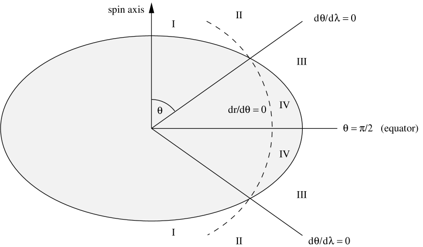
Figure 1.— Side view of a rotating neutron star (solid curve). Photons emitted from a point on the star at an angle $\theta$ from the spin axis can be emitted into regions I, II, or III if the star’s surface is an oblate spheroid. If the star’s surface is spherical (shown as a dashed curve), photons can only be emitted into regions II, III, or IV.

Integration of a single null ray proceeds by setting the initial coordinates $\bar{r}_{i}$ and $\theta_{i}$, selecting an allowed value of $b$, selecting an allowed value $\dot{\theta}_{i}$ according to the above prescription of the geometric constraints, and fixing $\dot{\bar{r}}_{i}^{2}$ and the sign of $\dot{\bar{r}}_{i}$ by the momentum and geometric constraints. The differential equations (2), (3), (4), and (5) are then integrated numerically until the radial coordinate reaches a predetermined large value.

2.3. Redshift and Zenith Angle

In CLM we presented equations for the photon’s redshift and initial zenith angle as measured in the frame co-rotating with the fluid for the case of photons emitted from and into the equatorial plane. The equations for arbitrary initial conditions are derived in a similar manner. The star’s fluid has four-velocity $u^{a}_{\star}=(t^{a}+\Omega_{\star}\phi^{a})/N_{\star}$ where the normalization function has the value

$$N_{\star}^{2}=e^{\gamma+\rho}\left(1-v_{Z}^{2}\right).$$ (14)

where

$$v_{Z}=(\Omega_{\star}-\omega)e^{-\rho}\bar{r}\sin\theta$$ (15)

is the speed of the star’s fluid as measured by a zero angular momentum observer.

Using $\ell^{a}$ to denote the photon’s four-velocity (as defined in section 2.1), the photon’s redshift as measured by an observer at infinity is given by $1+z=-u_{\star}\cdot\ell$, where we use a “dot” to denote the inner product with respect to the full 3+1 spacetime metric given in equation (1). The photon redshift is then

$$1+z=e^{-\frac{1}{2}(\gamma+\rho)}\frac{(1-\Omega_{\star}b)}{\sqrt{1-v_{Z}^{2}}}.$$ (16)

where all quantities are evaluated at the initial location on the star,

An inertial observer at infinity measures time using the $t$ coordinate, so the star’s spin period is $2\pi/\Omega_{\star}$. An inertial observer sitting at the star’s surface measures time with the local proper time $\tau$, where the proper and coordinate times are related by

$$\frac{d\tau}{dt}=e^{\frac{1}{2}({\gamma+\rho})}\sqrt{1-v_{Z}^{2}}.$$ (17)

The observer at the star’s surface measures the spin period to be gravitationally blue-shifted by the factor $d\tau/dt$.

Given a point on the surface of the star, the normal vector $n^{a}$ to the surface is defined by

$$n^{\bar{r}} = 1$$ (18)

$$n^{\theta} = -\frac{\bar{r}_{s}^{\prime}(\theta)}{\bar{r}_{s}^{2}}.$$ (19)

The angle between the initial photon direction and this normal, as measured in the star’s corotating frame is given by

$$\cos\alpha_{e}=\frac{n^{a}\ell^{b}h_{\star ab}}{n_{\star}\ell_{\star}}$$ (20)

where $h^{ab}_{\star}=g^{ab}+u^{a}_{\star}u^{b}_{\star}$ gives the projection of four-vectors to the 3-space defined for an observer rotating with the star, and $n_{\star}=h_{\star ab}n^{a}n^{b}$ and $\ell_{\star}=h_{\star ab}\ell^{a}\ell^{b}$. With these definitions, the angle $\alpha_{e}$ is

$$\cos\alpha_{e}=\frac{e^{\alpha}}{(1+z)}{\left(\dot{\bar{r}}-\dot{\theta}{\bar{r}_{s}^{\prime}}(\theta)\right)}{\left(1+\left(\frac{\bar{r}_{s}^{\prime}(\theta)}{\bar{r}_{s}}\right)^{2}\right)^{-1/2}}.$$ (21)

In this equation, $\dot{\bar{r}}$ and $\dot{\theta}$ are the initial values of the photon’s velocity components subject to the constraints given in section 2.2.

2.4. Doppler Factors

We expect that in the limit of slow rotation that the full formalism presented in this paper should reduce to the S+D approximation. In order to show that this is the case, we require the calculation of the special relativistic factors that enter into the Doppler shift formula. The Lorentz “boost” factor $\eta$ is defined by

$$\eta=\frac{\sqrt{1-v^{2}}}{1-v\cos\xi}$$ (22)

where $v$ is the speed of the emitting area, as measured by an inertial observer at the star, and $\xi$ is the initial angle between the fluid velocity and the initial photon direction, as measured by the inertial observer.

The inertial observer has four-velocity $u^{a}_{i}=t^{a}/N_{i}$, where the normalization factor is given by $N_{i}=e^{\frac{1}{2}(\gamma+\rho)}\left(1-\omega^{2}e^{-2\rho}\bar{r}^{2}\sin^{2}\theta\right)^{1/2}$. The spatial projection operator for this observer is $h_{i}^{ab}=g^{ab}+u^{a}_{i}u^{b}_{i}$, allowing the speed of the emitting area to be defined through the relation

$$v = \frac{(h_{iab}u^{a}_{\star}u^{b}_{\star})^{1/2}}{|u_{i}\cdot u_{\star}|}$$ (23)

$$= \Omega_{\star}e^{-\rho}\bar{r}\sin\theta(1-\omega(\Omega_{\star}-\omega)e^{-2\rho}\bar{r}^{2}\sin^{2}\theta)^{1/2}$$

The angle $\xi$ is defined by

$$\cos\xi=\frac{h_{iab}u^{a}_{\star}\ell^{b}}{(h_{iab}u^{a}_{\star}u^{b}_{\star})^{1/2}(h_{iab}\ell^{a}\ell^{b})^{1/2}},$$ (24)

which leads to the expression

$$1-v\cos\xi=\frac{\left(1-e^{-2\rho}\bar{r}^{2}\sin^{2}\theta\omega^{2}\right)}{\left(1-e^{-2\rho}\bar{r}^{2}\sin^{2}\theta\omega(\omega-\Omega_{\star})\right)}(1-\Omega_{\star}b).$$ (25)

We wish to make contact with the S+D approximation, in which the exterior gravitational field of the star is approximated by the Schwarzschild metric. The limiting values of the metric potentials for zero rotation were given by equations (3) - (5) of CLM. As discussed in CLM, the S+D approximation can be found by taking the limit of the frame-dragging potential $\omega$ to zero and using the Schwarzschild limits for the potentials $\gamma,\rho$ and $\alpha$. We will denote the S+D approximation of any expression with the limit $\omega\rightarrow 0$. In this limit, the values of $v$ and $v_{Z}$ are

$$\lim_{\omega\rightarrow 0}v=\lim_{\omega\rightarrow 0}v_{Z}=\frac{\Omega_{\star}R\sin\theta}{\sqrt{1-2M/R}},$$ (26)

and the Doppler Boost factor is

$$\lim_{\omega\rightarrow 0}\eta=\frac{\sqrt{1-v^{2}}}{1-\Omega_{\star}b}.$$ (27)

¿From equation (16) it can be seen that the redshift factor in the S+D approximation reduces to the expected expression

$$\lim_{\omega\rightarrow 0}(1+z)=(1-\frac{2M}{R})^{-1/2}\eta^{-1}.$$ (28)

2.5. Time of Arrival and Azimuthal Deflection Angle

The coordinate time of arrival for each photon is denoted $T$ and can be found by integrating equation (2) and subtracting off the time of arrival for some arbitrarily chosen reference photon. Similarly, the azimuthal deflection angle $\psi$ (the change in $\phi$ coordinate) can be found by integrating equation (3). Both the time of arrival and the azimuthal deflection angle can be written as functions of the photon’s initial latitude on the star $\theta_{i}$, the final latitude of the photon $\theta_{f}$ and the photon’s impact parameter $b$.

Consider the family of photons all emitted from the same latitude on the star, and all received by the same observer at infinity. These photons all have different values of $b$, and their times of arrival will be written as $T(\theta_{i},\theta_{f},b)$ and their azimuthal deflection is $\psi(\theta_{i},\theta_{f},b)$. If $\theta_{i}$ and $\theta_{f}$ are fixed, two photons with impact parameters $b$ and $b+\Delta b$ have times of arrival differing by

$$\Delta T=\frac{dT}{db}\Delta b.$$ (29)

The deflection angles for the two photons differ by

$$\Delta\psi=\frac{d\psi}{db}\Delta b.$$ (30)

In the Appendix, we show that $dT/db=bd\psi/db$. This leads to the identity, for photons with identical initial and final latitudes

$$\Delta T(\theta_{i},\theta_{f},b)=b\Delta\psi(\theta_{i},\theta_{f},b).$$ (31)

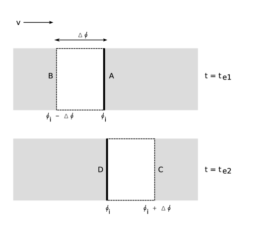
Figure 2.— An emitting region with azimuthal width $\Delta\phi$ which moves across the star at constant latitude. Photons from locations A and B are emitted simultaneously at time $t_{e1}$ and later, at time $t_{e2}$, photons C and D are emitted.

Consider two points on the same latitude of the star separated by an azimuthal angle $\Delta\phi$ as shown in Figure 2. As the star rotates, the azimuthal locations of the two points change, but the separation remains fixed. Suppose that photons are emitted simultaneously from the two points so that the leading photon (labeled “A”) has impact parameter $b$ and is emitted at some initial azimuthal angle $\phi_{i}$, and the trailing photon (labeled “B”) has impact parameter $b+\Delta b$ and initial azimuthal angle $\phi_{i}-\Delta\phi$. (In our sign convention the impact parameter is positive on the blue side of the star, and the azimuthal coordinate $\phi$ is negative on the blue side. With this sign convention $\Delta\phi$ is always positive.) Define the time of arrival for the leading photon to be $T_{A}$. Then the time of arrival for the trailing photon is $T_{B}=T_{A}+b\Delta\phi$ since $\Delta\phi=-\Delta\psi$. With our sign convention, on the blue side of the star $T_{B}>T_{A}$, so that the leading photon arrives before the trailing photon. On the red side of the star the opposite is true.

The location of the two emitting points at a coordinate time $\Delta t_{e}$ later is shown in the second panel of Figure 2. In this time interval each point has moved through an angle $\Delta\phi$, so the lapse in coordinate time is $\Delta t_{e}={\Delta\phi}/{\Omega_{\star}},$ where the subscript $e$ is used to denote the lapse in coordinate time measured at the location of the emitting points. The two photons emitted simultaneously at this later time are now labeled “C” (for the leading photon) and “D” (for the trailing photon). The trailing photon arrives at time

$$T_{D}=\frac{\Delta\phi}{\Omega_{\star}}+T_{A}$$ (32)

and the leading photon arrives at time

$$T_{C}=T_{D}-b\Delta\phi=T_{A}+\frac{\Delta\phi}{\Omega_{\star}}\left(1-b\Omega_{\star}\right).$$ (33)

The observer sees the photons move through the angle $\Delta\phi$ in the time interval $\Delta T$,

$$\Delta T=T_{C}-T_{A}=\frac{\Delta\phi}{\Omega_{\star}}\left(1-b\Omega_{\star}\right)=\Delta t_{e}\left(1-b\Omega_{\star}\right).$$ (34)

2.6. Solid Angle

The flux detected from an emitting area on the star is directly proportional to the solid angle subtended by the area, as measured by the observer. Consider any three photons arriving at the detector. Since the observer is located in a flat region of space, the solid angle can be found by first calculating the three angles separating the three photons. These three angles form a triangle whose area can be computed using Euclidean geometry.

Consider two photons seen by the observer with four-momenta $\ell$ and $m$ which has components $\ell_{t}=m_{t}=-1$, $\ell_{\phi}=b$, $m_{\phi}=b+db$, $m^{\theta}=\ell^{\theta}+d\ell^{\theta}$ and $m^{\bar{r}}=\ell^{\bar{r}}+d\ell^{\bar{r}}$. The angle between these two photons, as measured by a static observer at infinity can be found using a method similar to the Appendix of CLM, except that we now allow for photons detected and emitted off of the equator. After some algebra, the angle $\epsilon$ is given by

$$\cos(\epsilon)=1+g_{tt}\left[g^{\phi\phi}(\mathrm{d}b)^{2}+g_{\bar{r}\bar{r}}(\mathrm{d}\ell^{\bar{r}})^{2}+g_{\theta\theta}(\mathrm{d}\ell^{\theta})^{2}\right].$$ (35)

For small angular separations, $\cos(\epsilon)=1-\epsilon^{2}/2+\mathcal{O}(\epsilon^{4})$, so the angle separating the photons is

$$\epsilon=\sqrt{-g_{tt}}\left[g^{\phi\phi}(\mathrm{d}b)^{2}+g_{\bar{r}\bar{r}}(\mathrm{d}\ell^{\bar{r}})^{2}+g_{\theta\theta}(\mathrm{d}\ell^{\theta})^{2}\right]^{1/2}.$$ (36)

Given the three angles $\epsilon_{i}$ (where $i$ runs from 1 to 3) separating the three photons, the solid angle subtended by the photons can be found (assuming flat space at infinity) from a Euclidean formula such as

$$d\Omega=\sqrt{s(s-\epsilon_{1})(s-\epsilon_{2})(s-\epsilon_{3})},$$ (37)

where $s=(\epsilon_{1}+\epsilon_{2}+\epsilon_{3})/2$.

In our calculations, we must be careful about whether the photons were emitted or detected simultaneously. We use $d\Omega_{e}$ to denote the solid angle subtended by photons that were emitted simultaneously, but detected at different times. The solid angle subtended by photons that are detected simultaneously but emitted at different times is denoted $d\Omega_{o}$.

2.7. Light Curves

In order to construct a light curve, the flux as a function of observed coordinate time must be calculated. Consider two different instantaneous definitions of the flux from a small spot on the star with width $\Delta\phi$. The specific flux detected at time $T$ is

$$F_{o}(T)=\frac{I_{\nu_{e}}(\alpha_{e})}{(1+z)^{3}}d\Omega_{o},$$ (38)

where the values of $z$ and $\alpha_{e}$ have been chosen so that the photons arrive at the observer at the correct time. The flux received in the detector over a time interval due to photons emitted simultaneously at the same value of coordinate time $t_{e}$ is

$$F_{e}(t_{e})=\frac{I_{\nu_{e}}(\alpha_{e})}{(1+z)^{3}}d\Omega_{e}.$$ (39)

However, neither definition of flux describes what is truly measured in the detector, since the detector measures flux over a finite time interval $\Delta T$. Light detected during the interval $\Delta T$ is emitted over the coordinate time interval $\Delta t_{e}$, so the total energy per unit area that arrives in the detector is

$$\hbox{Total Energy}=F_{e}(t_{e})\Delta t_{e},$$ (40)

where we are now integrating the specific flux over all energies. The flux in the detector is averaged over the collection time interval $\Delta T$, so the measured flux is

$$F(T,\Delta T)=\frac{\hbox{Total Energy}}{\Delta T}=F_{e}(t_{e})\frac{\Delta t_{e}}{\Delta T}.$$ (41)

Making using of equation (34), the expression for the flux reduces to $F(T,\Delta T)=F_{e}(t_{e})/(1-b\Omega_{\star})$. In the S+D approximation (see equation (27)) this yields

$$\lim_{\omega\rightarrow 0}F(T,\Delta T)=F_{e}(t_{e})\eta,$$ (42)

as derived using other methods by Poutanen & Gierliński (2003).

In CLM we erroneously omitted the extra boost factor derived in this section. As a result, the pulse shapes shown in that paper are not correct. This means that in CLM we underestimated the errors introduced by neglecting time delays into the S+D fitting program. However, the conclusions made by CLM are unchanged: for equatorial photons, the most important effect is the binning of photons by the correct arrival time.

2.8. Approximation Schemes

The raytracing procedure discussed in this section is time-consuming, so simpler approximations based on analytic spacetime metrics are desirable. Two approximations are commonly used, the Schwarzschild + Doppler (S+D), and the Spherical Kerr (SK) approximations. In both of these approximations a black hole metric with a mass identical to the neutron star’s mass is used instead of the neutron star metric. In the case of the SK approximation, a Kerr metric with angular momentum identical to the neutron star’s is used. In both cases, photon trajectories are started from a spherical surface with a radius equal to the neutron star’s equatorial radius.

Another type of approximation retains the oblate shape of the rotating neutron star and embeds the oblate surface in either a Schwarzschild or Kerr spacetime metric. We will use the name Oblate Schwarzschild (OS) to denote the use of a Schwarzschild metric and an oblate surface, and Oblate Kerr (OK) for the use of the Kerr metric and an oblate surface.

3. Comparison of Methods

We now turn to the question of how well the various approximations model the light curves produced by rapidly-rotating neutron stars. We examine three aspects of this question. First, we address the effect of the shape of the star’s surface on the resulting light curve. Second, we address how the effect of the choice of metric affects the resulting light curve. Third, we examine the errors that result when the commonly adopted S+D approximation is used to extract the neutron star’s mass and radius values.

3.1. Oblate Shape of the Star

The most important factor affecting the light curve of a very rapidly-rotating neutron star is the assumed shape of the star’s surface. The reason for this can be seen in Figure 1, which shows emission from a point at an angle $\theta$ from the star’s spin axis. In Figure 1, the true shape of the star (an oblate spheroid) is shown, along with a spherical surface that intersects the point of emission. In Figure 1, four regions I, II, III, and IV are shown. If the star’s shape is either spherical or oblate, photons can always be emitted into regions II and III. However, in the case of a spherical star, region I is forbidden, and in the case of an oblate star, region IV is forbidden. If the star is very oblate, the differences in allowed initial directions can have a very dramatic effect on the resulting light curve.

Figure 3.— Light curves for a 600 Hz, 1.4 $M_{\odot}$ neutron star with EOS L, emission from an angle of $41^{\circ}$ from the North pole and an observer at an inclination angle of $20^{\circ}$ from the North pole. The bold solid curve is the light curve that results if the exact shape and gravitational field of the star is used. The four approximation schemes discussed in the text are shown in various types of dashed lines. Note that the OS and OK curves are very close to the exact curve and may be difficult to distinguish from the exact case.

In Figure 3 we show an example for the most oblate star, corresponding to EOS L with a mass of $1.4M_{\odot}$ and a spin frequency of 600 Hz. In Figure 3 we show the light curves which result if the emission takes place at an angle of $41^{\circ}$ from the spin axis, and the observer’s inclination angle is $20^{\circ}$ from the spin axis. The curve labeled “Exact” was computed using the exact numerical metric and the correct, oblate shape of the star. The curves labeled “OS” and “OK” were calculated by embedding the exact oblate shape in either the Schwarzschild or Kerr metrics respectively. These three curves are very close to each other and are difficult to distinguish. The curves labeled “S+D” and “SK” are computed by assuming a spherical shape for the star and evolving the photons in either a Schwarzschild or Kerr spacetime. The S+D and SK curves are very close to each other, and are very different in shape from the curves computed using the oblate surface. The curves computed in the spherical approximations are more modulated and have a higher harmonic content than the curves computed using either the oblate or exact methods. This is purely a geometric effect. Consider the situation when the spot is on the opposite side of the star from the observer. In the case of a spherical star the light must be emitted close to tangent to the surface in order to get to the observer. In the case of an oblate star, the same initial light ray is emitted closer to the normal to the surface. The solid angle subtended by the spot is roughly proportional to $\cos\alpha_{e}$. Since the brightness of the spot at any time is roughly approximate to the solid angle subtended by the spot, the spot’s brightness when it is on the far side of the star is larger in the oblate case than in the spherical case. This leads to less modulation in the case of an oblate star compared to a spherical star.

Figure 4.— Light curves for a 600 Hz, 1.4 $M_{\odot}$ neutron star with EOS L, emission from an angle of $15^{\circ}$ from the North pole and an observer at an inclination angle of $100^{\circ}$ from the North pole.

In Figure 4 we show a similar set of curves for the same star shown in Figure 3, but for emission from an angle of $15^{\circ}$ from the spin pole and an observer inclination of $100^{\circ}$. The differences between the curves for spherical and oblate stellar surfaces are even more extreme than in Figure 3. In Figure 4, the light curves assuming a spherical surface show eclipses, while the oblate light curves do not have eclipses. In the spherical cases, the eclipses occur when light from the back of the star would need to be emitted into region I (see Figure 1) in order to go over the north end of the star to reach the observer. Since region I is forbidden when the emission is from a spherical surface, eclipses occur. In the case of an oblate star, region I is allowed and light reaches the observer and no eclipse occurs.

Figure 5.— Light curves for a 600 Hz, 1.4 $M_{\odot}$ neutron star with EOS A, emission from an angle of $15^{\circ}$ from the North pole and an observer at an inclination angle of $100^{\circ}$ from the North pole.

Neutron stars constructed with EOS L are very large, so they are strongly affected by rotation and are very oblate. We have chosen to focus on EOS L in order to illustrate the largest changes to the waveforms caused by rotation. In contrast, a softer EOS, such as EOS A produces a smaller star that is less oblate. In Figure 5 we show the light curves for the same emission geometry as in Figure 4 but for EOS A. Note that in the case of the smaller EOS A star, there are no eclipses when the spherical surface approximation is made. The shapes of the light curves constructed with elliptical and spherical models are similar to each other, but the curves constructed with the spherical approximation are more modulated (for the same reasons as given for the case shown in Figure 3. The lack of eclipses for the spherical star is due to the fact that the EOS A star is much more compact than the EOS L star (with the same mass). A more compact star has a stronger gravitational field and the effect of light bending is much stronger than for a large star, so that it is easier for light to travel from the back side of the star to the observer. For the remaining figures we have chosen to focus on the larger EOS L stars in order to show the largest possible effects due to oblateness, but it should be remembered that if the EOS is softer, then the differences between the waveforms computed using the oblate and spherical models will be smaller than shown.

Figure 6.— Light curves for 1.4 $M_{\odot}$ neutron stars with EOS L, emission from an angle of $15^{\circ}$ from the North pole and an observer at an inclination angle of $100^{\circ}$ from the North pole. Light curves for spin rates of 100, 300 and 500 Hz are shown. Exact light curves are illustrated with bold curves. For comparison the approximate Schwarzschild + Doppler (S+D) light curves are also shown. The S+D and exact light curves for the 100 Hz star overlap, so the S+D curve can’t be distinguished from the exact in this figure.

In order to illustrate the effect of rotation rate on the light curves, we plot in Figure 6 the light curves for emission from an angle of $15^{\circ}$ and detection at $100^{\circ}$ for stars rotating at frequencies 100, 300 and 500 Hz. For the case of the 100 Hz star (solid lines) the exact (bold) and approximate S+D (light) curves are almost identical and are difficult to distinguish from each other in Figure 6. Since 100 Hz is a relatively slow rotation rate and oblateness is small, the S+D light curve is an excellent approximation to the exact light curve. The light curves for 300 Hz stars (dot-dashed lines) show a significant difference between the exact (bold) and S+D (light) curves. In both cases (for 300 Hz) the spot is eclipsed, but for the exact light curve the eclipse lasts for about 1/10 of the spin period, while in the S+D approximation the eclipse lasts for about 2/10 of the spin period. In the case of 500 Hz (dotted lines) the exact light curve (bold) has no eclipse while the S+D approximation (light) does, as in the case of 600 Hz.

Figure 7.— Light curves for a 600 Hz, 1.4 $M_{\odot}$ neutron star with EOS L, emission from an angle of $85^{\circ}$ from the North pole and an observer at an inclination angle of $100^{\circ}$ from the North pole.

When emission and detection takes place near the star’s equatorial plane the differences in the light curves resulting from the different calculation methods are not as important, as shown in Figure 7. In Figure 7 emission is from a point $85^{\circ}$ from the spin pole and the observer has an inclination angle of $100^{\circ}$. While the fraction of the time that the signal is “on” is different for the oblate and spherical cases, the difference is not very important. This lack of difference is due to the fact that near the equator, there is not much difference between the normals to an oblate spheroid or a sphere. This agrees with the earlier results in CLM for the case of exact equatorial orbits.

Figure 8.— Light curves for a 600 Hz, 1.4 $M_{\odot}$ neutron star with EOS L, emission from an angle of $45^{\circ}$ from the North pole and an observer at an inclination angle of $135^{\circ}$ from the North pole.

When the observer and the emission region are on opposite sides of the star, as in the case of Figure 8), the effect of oblateness is to increase the duration of eclipses compared to an equivalent light curve computed with a spherical surface. The reason for this can be understood by considering the case of a spherical star. For the spherical star, the eclipse begins at the moment that the light is emitted tangent to the surface, into region IV of Figure 1. But the oblate star is not allowed to emit into region IV, so this photon never reaches the observer. This analysis holds for all photons that would have to be emitted into region IV, with the result that the eclipse lasts for a longer time in the case of the oblate star. In general, this leads to a higher asymmetry and harmonic content for light curves for the oblate star (compared to the spherical star) if the angles of emission and detection are in opposite hemispheres.

Since neither the oblateness of the star nor the emission and detection angles are typically known for any observation, the use of one of the spherical approximations for a rapidly-rotating neutron star can lead to incorrect fits.

3.2. Metric Approximations

Given an initial photon direction, the most important factor of affecting the propagation of a photon is the strength of the gravitational potential at the location of emission. To leading order in rotation, the gravitational potential depends only on the ratio of $M/R$. Approximations using the Schwarzschild metric to model the neutron star’s gravitational field assume that the value of $M/R$ predicts the deflection and time delay of the photons at a level sufficient for light-curve fitting.

The largest rotational correction to the star’s metric is the frame-dragging term $\omega$ which is of order $\Omega_{\star}\times M/R$. The use of the Kerr metric matches the neutron star’s metric up to this first order rotational term, but does not attempt to match the exact metric at quadratic order (or higher) in the angular velocity.

In Figures 3, 4 and 7 we showed the light curves that result when the Schwarzschild and Kerr approximations are used. The differences between the choice of metric are smaller than the differences caused by the shape of the initial emission surface in the cases illustrated in Figures 3 and 4. In the case of Figure 7, all of the curves are so close that the approximation scheme is unimportant. The uncertainties in the shape and size of the emission area, along with the uncertainty in the anisotropy of the emission will produce uncertainties in the shapes of the light curves which are much larger than the differences in light curves caused by the choice of metric. However, the errors caused by using the wrong shape of the surface are competitive with the differences caused by uncertainties in the emission shape, size and anisotropy.

As a result, we find no compelling reason to make use of the Kerr metric over the Schwarzschild metric. An approximation scheme such as the OS results in light curves that approximate the exact curves about as well as the OK approximation.

3.3. Errors in Fitted Masses and Radii for the S+D Approximation

The main motivation for calculating light curves is to extract the neutron star’s mass and radius. At present the only methods for fitting the mass and radius from light curves approximate the star’s surface as a sphere. We now give results of a preliminary investigation of the errors in fitted mass and radius resulting from the use of a spherical approximation. First, light curves are created using the exact (numerical) description of the neutron star for a number of different stellar models, emission latitudes and observer inclination angles. We then used a S+D fitting program to deduce the mass and radius of the stars as well as the emission-observer geometry given the pulse shape and the star’s spin frequency. In order to isolate the effects of oblateness on the errors, we only used infinitesimal spot sizes and isotropic emission in both the exact curve generating program and in the S+D fitting program. This method provides a first clue to the effects of oblateness, but in order to model real data a fitting program should be allowed to explore a larger parameter space including finite spot size, complicated spot patterns and anisotropic emission.

The results of the fits are shown in Table 2. In all cases the true value of the star’s mass is $1.4M_{\odot}$. In this table, the term $R(\theta_{e})$ is displayed. When the S+D fitting program fits values, the light bending and Doppler boosts depend on the value of the radius at latitude of the spot, not at the equator. This means that when the S+D fitting program fits the star’s radius, it is actually predicting $R(\theta_{e})$ the radial distance from the centre of the star to the fitted location of the spot. In the column labeled “$R(\theta_{e})$ true”, this is the distance from the centre of the star to the actual location of the spot. Similarly, the true and fitted values of the gravitational potential at the location of emission $M/R(\theta_{e})$ are shown in the table.

The S+D fitting is done by selecting a value of $M/R$ at the location of emission. This fixes the bending angles and times of arrival in the Schwarzschild metric. Different values of $R$ and the emission and observer angles are tried, which fix the Doppler boosts, since the star’s spin frequency is assumed to be known. A light curve is calculated and compared to the light curve computed by the exact method, and the $\chi^{2}$ value is calculated assuming constant error per data point of 0.01, with the data normalized so that the peak of the light curve equals 1.

In the S+D light curves 180 phase bins are used. The mean counts per bin ranges from .15 to .7, with peak normalized to 1.0. The error of 0.01 per phase bin is, using Poisson errors, equivalent to a 220 to 500 counts per bin or a total of 40,000 to 90,000 counts. These errors are comparable to those that can be obtained on ms pulsars using the Rossi X-ray Timing Explorer. For example, one of the best statistics is for the light curves shown in Papitto et al (2005). They show pulse shapes (mean normalized to 1.0) of SAX J1808.4-3658 with 64 phase bins and errors per phase bin of 0.005, which implies 40,000 counts per bin for a total of 2.6$\times 10^{6}$ counts. The number of degrees of freedom in our fits is 180-NP with NP=6 the number of fit parameters. Since the S+D model light curve was fitted to exact light curve without added Poisson errors, the expected $\chi^{2}$ for a perfect fit is 0 rather than 180-NP. Given the assumed errors of 0.01 per phase bin, $\chi^{2}$ values of 1, 2.71 and 4 roughly correspond to inconsistency of model and input light curves at the 1$\sigma$, 90$\%$, and 2$\sigma$ levels.

After the minimum $\chi^{2}$ value ($\chi^{2}_{min}$) is found, the best values of the star’s radius at the point of emission and the angles $\theta_{e}$ and $\theta_{o}$ given the value of $M/R$ is known. The process is then repeated for a new value of $M/R$. By iterating this for many values of $M/R$, the best fit model can be found. In Table 2, the best fit parameters are shown for each light curve, along with the 90$\%$ uncertainty in the fitted value of $M/R$ and the value of $\chi^{2}_{min}$ for the best-fit model. The uncertainty is computed by finding the values of $M/R$ which yield $\chi^{2}$=$\chi^{2}_{min}$+2.71. We allowed all other parameters to be free in the fits to find the range of parameter of interest which gave $\chi^{2}$=$\chi^{2}_{min}$+2.71. Thus there have been no assumptions about correlations between parameters, and we have found the correct $90\%$ ranges. In some cases, the minimum in $\chi^{2}$ is so shallow that no meaningful error bars can be computed. We denote these cases with an asterisk in the uncertainty column. The cases marked with an asterisk are degenerate, in that almost any values of $M/R$ provides an acceptable fit to the data. In some other cases (see emission angle of 45°, observation angle of 135°and EOS L) the error bars allowed an upper limit on $M/R$ to be made. In these cases the uncertainty column contains the symbol “$<$” and a number which is the upper limit on $M/R$. Computing $90\%$ uncertainties for the other parameters than $M/R$ is beyond the scope of this paper. One might expect that in cases where the fits are not degenerate the errors should be of roughly similar fractional amount as for $M/R$, however more work is required to confirm this.

The fit value of $M/R$ often agree closely (within 5%) with the true $M/R$ values. Eleven (8 degenerate, 3 non-degenerate) of the fits had M/R fit different than $M/R$ true by 10$\%$ to 50$\%$, another 3 had differences between 5 and 10$\%$. If we discount the degenerate fits, that leaves 6 out of 30 cases with errors between 5$\%$ and 21$\%$. Thus the S+D approximation does have a small but significant (20$\%$) fraction of cases with significant errors in $M/R$. For the remaining parameters ($M$, $R$ and the angles $\theta_{e}$, $\theta_{o}$) the differences between the true and fit values are larger than for the ratio $M/R$, with usually larger differences for the angles than for $M$ or $R$. For example the fit values of $M$ are different than the true values by by 10$\%$ to 24$\%$ in 10 cases (out of 30 nondegenerate fits), and 11 cases had differences between 5 and 10$\%$. For $\theta_{e}$, fit values are different than the true values by by 10$\%$ to 98$\%$ in 16 cases (out of 30 nondegenerate fits), and 6 cases had differences between 5 and 10$\%$. Generally, we find that the errors in using the S+D approximation can be large in some cases and small in some others. However, one must be careful in interpreting the results of this work: for real data, as previously mentioned, one would have to generalize the study to include a finite spot size and more realistic emissivity.

Table 2 illustrates a number of types of fitting problems that occur. For the slowest rotating stars with spin frequencies $\nu_{star}\leq 200$ Hz, the S+D fitting program extracted a value of $M/R$ very close to the actual value, as would be expected for slowly rotating stars. The individual fitted values of mass and radius have some error, but don’t deviate by more than 6% from the true values. In order to fit the radius of the star, the equatorial velocity is fit from the asymmetry in the light curve due to Doppler boosting. At slow rotation rates the effects of Doppler boosting is small and the exact light curves have fairly symmetric rise and fall times. The result is that due to this symmetry a range of radii will fit the data equally well, leading to a high probability that some error will be introduced into the fitted value of radius. As the spin rate is increased, the quality of the fits (as measured by $\chi^{2}$) decreases, but the resulting fits for $M/R$ are (within the error) of the correct values of $M/R$ when the spin frequency is $\leq 500$ Hz. However, the fits for the masses (or radius) are quite poor in many of these cases.

In the case of emission from 41°and observation at 20°all fits at all spin frequencies were degenerate (although we only chose to show a few of these in Table 2). This can be understood by looking at the light curve (for the case of 600 Hz) shown in Figure 3. The true light curve for this angle combination is very close to a sine wave at all spin frequencies. Since almost any star will have a number of emission/observation angle pairs that produce a sine wave signal, a wide range of model stars provide equally good fits to the data. As others (eg. Bhattacharyya et al. (2005)) have remarked, any data which does not contain any harmonics will not allow meaningful fits.

Some of the worst errors in extracting mass and radius occur for the largest stars constructed with EOS L, one of the stiffest EOS in the literature. Since the EOS L stars are very large, they are most affected by rotation and are highly oblate. If one is interested in ruling out very stiff equations of state, using data from rapidly-rotating stars, it is necessary to take the oblateness of these stars into account.

4. Conclusions

We have investigated the effect of rapid rotation on the light curves produced by a small spot on a neutron star’s surface. Our calculations are exact, in that we numerically compute the spacetime metric for the rotating star, include the correct shape of the star and solve for the geodesics in the numerical spacetime. We find that the most important effect on the light curve arising from rotation comes from the oblate shape of the star’s surface.

All past work involving fits of X-ray data have assumed that the surface of the star is spherical. Our present computations show that the assumption of a spherical surface leads to large deviations from the correct light curve for spin frequencies larger than 300 Hz. However, our test runs show that the assumption of a spherical surface can still fit the correct value of $M/R$ at spin frequencies $\leq 500$ Hz, even if the individually fitted values of mass and radius are incorrect.

In our light curve calculations, we find that if the star’s surface is assumed to be a sphere, the light curves resulting from the use of the Kerr metric are almost the same as those resulting from the use of the Schwarzschild metric. The difference in these light curves is smaller than the size of the error bars in any present data, so it seems that there is no significant advantage in the use of the SK approximation over the S+D approximation.

We calculated light curves in an approximation where an oblate surface is embedded in either the Schwarzschild (OS) or Kerr (OK) spacetime. In both cases, the resulting light curves are very close to the exact light curves computed using the numerical spacetime of the rotating neutron star. This suggests that an approximation similar to the Schwarzschild + Doppler approximation that includes an oblate surface could be a useful way to fit data. The construction of a fitting program that extracts the mass and radius of a star from a light curve using an oblate surface is non-trivial. In future work, we plan to develop a code that will allow an oblate shape to be incorporated into a S+D fitting program that includes finite spot sizes and anisotropic emission. We anticipate that such a program will allow the accurate extraction of the masses and radii of very rapidly-rotating neutron stars.

Table 1Neutron Star Parameters for 1.4 $M_{\odot}$ Stars

EOS	$\nu_{*}$	$R$	$GM/Rc^{2}$	$Jc/M^{2}G$	$v/c$	$\nu_{B}$
	Hz	km				Hz
A	0	9.57	0.216	0	0	1390
	100	9.57	0.216	0.04	0.03
	200	9.59	0.216	0.07	0.05
	300	9.62	0.215	0.11	0.08
	400	9.66	0.214	0.15	0.11
	500	9.71	0.213	0.19	0.13
	600	9.78	0.211	0.22	0.16
L	0	14.8	0.139	0	0	740
	100	14.9	0.139	0.08	0.04
	200	14.9	0.138	0.15	0.07
	300	15.1	0.137	0.23	0.11
	400	15.4	0.135	0.32	0.15
	500	15.7	0.131	0.41	0.19
	600	16.4	0.126	0.51	0.24

Table 2Comparison of True and Fitted Parameters of Neutron Stars. All neutron stars have a mass of $1.4M_{\odot}$.

$\theta_{e}$	$\theta_{o}$	EOS	$\Omega_{\star}$ (Hz)	$M/M_{\odot}$	$R(\theta_{e})$ (km)		$\theta_{e}$ (deg)	$\theta_{o}$ (deg)	$GM/c^{2}R(\theta_{e})$			$\chi^{2}$
true				fit	true	fit	fit	fit	true	fit	unc.
41°	100°	A	100	1.48	9.57	10.2	80.5	139.2	0.216	0.215	0.011	0.1
		L		1.32	14.83	13.8	80.5	133.0	0.140	0.142	0.027	0.02
		A	300	1.49	9.58	10.0	79.8	138.0	0.216	0.220	0.005	1
		L		1.09	14.82	11.1	67.0	95.6	0.140	0.145	0.024	0.3
		A	400	1.45	9.58	9.55	80.8	134.9	0.216	0.225	0.006	2
		L		1.17	14.80	11.9	58.0	96.3	0.140	0.145	0.023	0.4
		A	500	1.51	9.59	9.89	80.2	136.9	0.216	0.225	0.005	3
		L		1.29	14.78	12.7	52.7	98.1	0.140	0.15	0.02	0.8
		A	600	1.58	9.60	10.2	41.9	102.2	0.215	0.230	0.007	4
		L		1.30	14.74	12.0	57.9	97.5	0.140	0.160	0.015	2
85°	100°	A	100	1.48	9.57	10.4	87.4	110.8	0.216	0.210	0.008	1
		L		1.45	14.86	15.3	84.0	103.7	0.139	0.140	0.027	0.05
		A	200	1.46	9.59	10.1	84.4	103.9	0.216	0.215	0.006	2
		L		1.43	14.95	15.6	86.7	107.6	0.138	0.135	0.029	0.4
		A	300	1.48	9.62	10.2	83.1	103.5	0.215	0.215	0.025	4
		L		1.70	15.10	17.9	80.0	123.3	0.137	0.140	0.015	0.4
		A	400	1.49	9.66	10.3	77.2	99.7	0.214	0.215	0.003	7
		L		1.40	15.35	16.0	85.0	105.5	0.135	0.130	0.009	4
		A	500	1.68	9.71	11.3	67.7	111.0	0.213	0.220	0.004	5
		L		1.51	15.73	17.9	61.7	97.7	0.131	0.125	0.009	6
		A	600	1.62	9.78	11.1	72.5	113.6	0.211	0.215	0.003	0.1
		L		1.40	16.35	17.3	77.8	102.6	0.127	0.120	0.007	0.2
45°	135°	A	100	1.51	9.57	10.4	47.4	137.8	0.216	0.216	0.005	0.1
		L		1.46	14.83	15.4	44.8	135.4	0.139	0.140	$<0.155$	0.06
		A	200	1.60	9.58	10.9	45.5	138.5	0.216	0.218	0.004	1
		L		1.48	14.84	15.7	44.3	136.0	0.139	0.140	$<0.145$	0.1
		A	300	1.57	9.58	10.7	45.1	137.6	0.216	0.217	0.006	0.5
		L		1.45	14.85	15.9	44.0	136.0	0.139	0.135	$<0.155$	0.1
		A	400	1.73	9.59	11.6	41.6	139.0	0.216	0.220	0.005	8
		L		1.44	14.87	16.3	43.0	136.4	0.139	0.130	$<0.145$	0.1
		A	500	1.61	9.61	11.0	44.5	138.6	0.215	0.216	0.005	1
		L		1.22	14.81	18.0	32.0	123.4	0.139	0.100	$<0.135$	0.8
		A	600	1.63	9.63	11.2	42.5	137.7	0.215	0.215	0.005	1
		L		1.34	14.90	18.0	40.0	137.5	0.139	0.110	$<0.145$	0.6
41°	20°	A	100	1.41	9.57	9.23	29.8	28.9	0.216	0.225	*	0.005
		A	500	1.40	9.59	10.4	20.6	35.3	0.216	0.2	*	0.05
		L		1.99	14.78	16.8	33.2	21.5	0.140	0.175	*	0.03
		A	600	1.40	9.60	10.9	20.2	34.0	0.215	0.19	*	0.07
		L		2.53	14.74	17.8	28.8	23.2	0.140	0.21	*	0.06
15°	100°	A	100	1.08	9.57	6.35	30.1	80.9	0.216	0.25	*	4
		A	500	0.59	9.51	8.76	54.7	21.8	0.217	0.1	*	1
		L		0.85	14.25	8.41	30.2	78.1	0.145	0.15	*	0.8
		A	600	0.68	9.49	9.10	56.9	20.3	0.218	0.11	*	0.8
		L		0.92	13.98	7.98	34.1	69.5	0.148	0.17	*	2

Appendix A Relation Between Times-of-Arrival and Deflection Angles

In order to compute the coordinate time elapsed during the photon’s flight from the star to the observer, equation (2) must be integrated from the initial to final values of the affine parameter $\lambda$. This is complicated by the fact that the metric potentials $\gamma,\rho$ and $\omega$ appearing in equation (2) depend on the values of the coordinates $\bar{r}(\lambda)$ and $\theta(\lambda)$ describing the location of the photon at every point along the geodesic.

It is useful to introduce a flat, spacelike two-dimensional space perpendicular to the full $3+1$ spacetime’s Killing vectors. As the photon moves through the real spacetime it also traces out a curve in the two-space. The arc-length along the curve in the two-space is denoted $\zeta$ and is given by the usual flat space formula

$$d\zeta^{2}=d\bar{r}^{2}+\bar{r}^{2}d\theta^{2}.$$ (A1)

Since the arc-length depends on the value of the affine parameter $\lambda$, equation (7) can be used to write an equation for $\dot{\zeta}\equiv d\zeta/d\lambda$,

$$\dot{\zeta}^{2}={\mathcal{A}}(\bar{r}(\zeta),\theta(\zeta)).$$ (A2)

The elapsed coordinate time can now be written as the integral

$$T(\theta_{i},\theta_{f},b) = \int\frac{dt}{d\zeta}d\zeta=\int\frac{\dot{t}}{\dot{\zeta}}d\zeta=\int{{\mathcal{A}}^{-1/2}}{e^{-(\gamma+\rho)}(1-\omega b)}d\zeta.$$ (A3)

Similarly, the azimuthal deflection can be written as

$$\psi(\theta_{i},\theta_{f},b)=\int{{\mathcal{A}}^{-1/2}}\left({\omega e^{-(\gamma+\rho)}(1-\omega b)+e^{\rho-\gamma}\frac{b}{\bar{r}^{2}\sin^{2}\theta}}\right)d\zeta.$$ (A4)

Neither equation (A3) nor (A4) is in a form useful for directly calculating either the elapsed time or the azimuthal deflection. However, note that both of these equations are of the form of exact line integrals. If the value of the impact parameter is kept fixed, the values of the two integrals depend only on the endpoints. If the endpoints of the geodesic are kept fixed, the changes in the arrival time and in the azimuthal deflection angles can easily be calculated for small changes in the impact parameter. Making use of equations (6) and (7), the derivative of the coordinate arrival time with respect to the impact parameter is found to have the value

$$\frac{dT}{db} = \int{\mathcal{A}}^{-3/2}e^{-2\alpha-2\gamma}\frac{b}{r^{2}\sin^{2}\theta}d\zeta.$$ (A5)

Similarly, we find

$$\frac{d\psi}{db} = \int{\mathcal{A}}^{-3/2}e^{-2\alpha-2\gamma}\frac{1}{r^{2}\sin^{2}\theta}d\zeta.$$ (A6)

Comparing equations (A5) and (A6) we are led to the identity

$$\frac{dT}{db}(\theta_{i},\theta_{f},b)=b\frac{d\psi}{db}(\theta_{i},\theta_{f},b).$$ (A7)

As a result, if two photons are emitted from the same latitude $\theta_{i}$ on the star and are detected by the same observer, the difference in arrival times is related to the difference in the azimuthal deflection by the simple formula given by equation (A7).

As a quick check, we note that in the limit of zero rotation the metric potentials are given by equations (3 - 5) of Cadeau et al (2005), and the integrals for the time delay and azimuthal deflection reduce to simple integrals over the radial coordinate. It is easy to explicitly check that the identity (A7) holds in the case of the Schwarzschild metric, as it must since our proof holds for any axisymmetric stationary spacetime.

References

- Akmal et al. (1998) Akmal, A., Pandharipande, V. R., & Ravenhall, D. G. 1998, Phys. Rev. C, 58, 1804
- Arnett & Bowers (1977) Arnett, W. D., & Bowers, R. L. 1977, ApJS, 33, 415
- Bhattacharyya et al. (2005) Bhattacharyya, S., Strohmayer, T. E., Miller, M. C., & Markwardt, C. B. 2005, ApJ, 619, 483
- Bhattacharyya, Miller & Lamb (2006) Bhattacharyya, S., Miller, M. C., & Lamb, F. K. 2006, ApJ, 644, 1085
- Braje & Romani (2001) Braje, T. M., & Romani, R. W. 2001, ApJ, 550, 392
- Braje, Romani, & Rauch (2000) Braje, T. M., Romani, R. W., & Rauch, K. P. 2000, ApJ, 531, 447
- Cadeau, Leahy, & Morsink (2005) Cadeau, C., Leahy, D. A., & Morsink, S. M. 2005, ApJ, 618, 451
- Chakrabarty & Morgan (1998) Chakrabarty, D. & Morgan, E. H. 1998, Nature, 394, 346
- Chang et al. (2006) Chang, P., Morsink, S., Bildsten, L., & Wasserman, I. 2006, ApJ, 636, L117
- Chen & Shaham (1989) Chen, K. & Shaham, J. 1989, ApJ, 339, 279
- Cook, Shapiro, & Teukolsky (1994) Cook, G. B., Shapiro, S. L., Teukolsky, S. A. 1994, ApJ, 424, 823
- Ghosh & Lamb (1978) Ghosh, P. & Lamb, F. K. 1978, ApJ, 223, L83
- Hessels et al. (2006) Hessels, J. W. T., Ransom, S. M., Stairs, I. H., Freire, P. C. C., Kaspi, V. M., & Camilo, F. 2006, Science, 311, 1901
- Heyl (2004) Heyl, J. S., 2004, ApJ, 600, 939
- Heyl (2005) Heyl, J. S., 2005, ApJ, 361, 504
- Komatsu, Eriguchi & Hachisu (1989) Komatsu, H., Eriguchi, Y., &Hachisu, I. 1989, MNRAS, 237, 355
- Kulkarni & Romanova (2005) Kulkarni, A. K. & Romanova, M. M. 2005, ApJ, 633, 349
- Leahy (2004) Leahy, D. A. 2004, ApJ, 613, 517
- Lee & Strohmayer (2005) Lee, U. & Strohmayer, T. E. 2005, MNRAS, 361, 659
- Miller & Lamb (1998) Miller, M. C. & Lamb, F. K. 1998, ApJ, 499, L37
- Özel & Psaltis (2003) Özel, F. & Psaltis, D. 2003, ApJ582, L31-L34
- Papitto et al (2005) Papitto, A., Menna, M. T., Burderi, L., Di Salvo, T., D’Antona, F., & Robba, N. R. 2005, ApJ, 621, L113
- Pechenick, Ftaclas, & Cohen (1983) Pechenick, K. R., Ftaclas, C., & Cohen, J. M. 1983, ApJ, 274, 846
- Poutanen & Gierliński (2003) Poutanen, J. & Gierliński, M. 2003, MNRAS, 343, 1301
- Press et al. (1992) Press, W. H., Teukolsky, S. A., Vetterling, W. T., & Flannery, B. P. 1992, Numerical Recipes in C, Second Edition, Cambridge University Press
- Stergioulas & Friedman (1995) Stergioulas, N. & Friedman, J. L. 1995, ApJ, 444, 306
- Terrell (1959) Terrell, J. 1959, Phys. Rev., 116, 1041
- Villarreal & Strohmayer (2004) Villarreal, A. R., & Strohmayer, T. E. 2004, ApJ, 614, L121