On the inconsistency between the black hole mass function
inferred from $M_{\bullet}-\sigma$ and $M_{\bullet}-L$ correlations

Abstract

Black hole masses are tightly correlated with the stellar velocity dispersions of the bulges which surround them, and slightly less-well correlated with the bulge luminosity. It is common to use these correlations to estimate the expected abundance of massive black holes. This is usually done by starting from an observed distribution of velocity dispersions or luminosities and then changing variables. This procedure neglects the fact that there is intrinsic scatter in these black hole mass–observable correlations. Accounting for this scatter results in estimates of black hole abundances which are larger by almost an order of magnitude at masses $>10^{9}M_{\odot}$. Including this scatter is particularly important for models which seek to infer quasar lifetimes and duty cycles from the local black hole mass function. However, even when scatter has been accounted for, the $M_{\bullet}-\sigma$ relation predicts fewer massive black holes than does the $M_{\bullet}-L$ relation. This is because the $\sigma-L$ relation in the black hole samples currently available is inconsistent with that in the SDSS sample from which the distributions of $L$ or $\sigma$ are based: the black hole samples have smaller $L$ for a given $\sigma$, or larger $\sigma$ for a given $L$. The $\sigma-L$ relation in the black hole samples is similarly discrepant with that in other samples of nearby early-type galaxies. This suggests that current black hole samples are biased: if this is a selection rather than physical effect, then the $M_{\bullet}-\sigma$ and $M_{\bullet}-L$ relations currently in the literature are also biased from their true values.

1. Introduction

The abundance of supermassive black holes is the subject of considerable current interest (e.g. Yu & Tremaine 2002; Marconi et al. 2004; McLure & Dunlop 2004; Shankar et al. 2004; Yu & Lu 2004; Ferrarese & Ford 2005). Several groups have noted that galaxy formation and supermassive black holes growth should be linked, and many have modeled the joint cosmological evolution of quasars and galaxies (see, e.g., Monaco et al. 2000; Kauffmann & Haehnelt 2001; Granato et al. 2001; Cavaliere & Vittorini 2002; Cattaneo & Bernardi 2003; Haiman et al. 2004; Hopkins et al. 2006; Lapi et al. 2006; Haiman et al. 2006 and references therein). Since the number of black hole detections to date is less than fifty, their abundance is estimated by using secondary indicators. In particular, $M_{\bullet}$ is observed to correlate strongly and tightly with the velocity dispersion of the surrounding bulge (e.g. Ferrarese & Merritt 2000; Gebhardt et al. 2000; Tremaine et al. 2002). Since detecting bulges is considerably easier than detecting black holes, it has become common to estimate the abundance of black holes by combining the observed distribution of bulge velocity dispersions (e.g. Sheth et al. 2003) with the observed $M_{\bullet}-\sigma$ relation. A crude estimate follows easily if one is willing to assume that all bulges host black holes, and that the $M_{\bullet}-\sigma$ relation has no intrinsic scatter (e.g. Yu & Tremaine 2002; Aller & Richstone 2002).

There is some discussion in the literature about whether $L$ or $\sigma$ is a better predictor of $M_{\bullet}$. There are two parts to this statement which are not always stated explicitly. The first is the assumption that the $M_{\bullet}-$observable relation is a single power law; whether this is a better approximation for $L$ than for $\sigma$ is an open question, although Lauer et al. (2007) argue that the curvature in the $\sigma-L$ relation for massive early-type galaxies (Bernardi et al. 2007a; Bernardi 2007) suggests that the $M_{\bullet}-\sigma$ relation is unlikely to be a single power-law. In what follows, we will assume the relations in question are indeed single power laws.

The second is the issue of the scatter around the mean relations. It is generally believed that the relation with smaller scatter provides the better estimate of the $M_{\bullet}$ distribution. Indeed, Marconi et al. (2004) state that if the scatter around two relations is similar, then both relations should provide equivalent descriptions of the distribution of $M_{\bullet}$. One of the goals of the present paper is to show that this is not the whole story. Provided the intrinsic scatter around the two relations is accurately known, whether or not one relation is tighter than another is irrelevant. (The only practical difference is that, if the intrinsic scatter is smaller, then observations of fewer objects are required to estimate it reliably.)

Both the $M_{\bullet}-\sigma$ and $M_{\bullet}-L$ relations show considerable scatter, not all of which can be accounted-for by measurement errors. Marconi & Hunt (2003) present evidence that the amount by which an object scatters from these relations is correlated with bulge size (half light radius), suggesting that at least some component of the scatter is intrinsic. Gebhardt et al. (2000) suggest that the intrinsic scatter in $M_{\bullet}$ at fixed velocity dispersion is of order 0.25 dex, whereas scatter around $M_{\bullet}-L_{V}$ is about 0.35 dex (e.g. Novak et al. 2006). If the intrinsic scatter is indeed this large, then it must be accounted for, especially when estimating the abundances of the most massive black holes ($M_{\bullet}\geq 10^{9}\,M_{\odot}$).

Section 2 describes a toy model of the effects of scatter which shows that, (i) if intrinsic scatter is ignored, then both the $L$- and $\sigma$-based predictions will underestimate the true abundance of the most massive black holes; (ii) the observable which correlates most tightly with $M_{\bullet}$ will provide the best estimate of the true abundance of the most massive black holes; (iii) if scatter has been correctly accounted for, $\sigma$- and $L$-based predictors of $M_{\bullet}$ abundances should give the same answer. It then shows the $M_{\bullet}-\sigma$, $M_{\bullet}-L$ and $\sigma-L$ correlations, their scatter, and how we use them to estimate black hole abundances. A direct comparison of the luminosity and velocity dispersion based predictors is provided, both when intrinsic scatter in these relations is accounted for and when it is ignored.

We find that, if scatter is ignored, then the $L$-based method predicts substantially more $10^{9}M_{\odot}$ objects than does the $\sigma$-based method. The toy model suggests that this may be a consequence of ignoring the intrinsic scatter. However, accounting for this scatter does not eliminate this discrepancy, suggesting that there may be a more serious inconsistency. Section 3 identifies the reason for this discrepancy with the fact that the $\sigma-L$ relation in the SDSS/Bernardi et al. (2003a) (hereafter SDSS-B07; see Bernardi 2007 for the definition of the SDSS-B07 sample), from which the $L$ and $\sigma$ distributions are drawn, is rather different from that in the black hole samples, from which the $M_{\bullet}-\sigma$ and $M_{\bullet}-L$ relations are derived. A more detailed analysis of the role of selection effects in the $M_{\bullet}$ sample is presented in Bernardi et al. (2007b). A final section discusses our findings and summarizes our conclusions. A standard flat $\Lambda$CDM comological model has been used, with $\Omega_{m}=0.3$, $\Omega_{\Lambda}=0.7$ and $H_{0}=70$ km s^-1 Mpc^-1.

2. Black hole abundances from $M_{\bullet}$-observable correlations

The first part of this section discusses the effect of intrinsic scatter in $M_{\bullet}$-observable relations on inferences about black hole abundances. The second part shows various $M_{\bullet}$-observable correlations in the compilation of Häring & Rix (2004). The third and fourth parts of this section show the predicted black hole abundances when intrinsic scatter in these relations is accounted for and when it is not.

A detailed discussion of exactly how the black hole sample was compiled, as well as how we convert from B, V, R and I-band luminosities to SDSS $r-$band is provided in Appendix A of Bernardi et al. (2007b). Briefly, all luminosities and black hole mass estimates depend on distance: where necessary, these were computed by scaling results in the literature to $H_{0}=70$ km s^-1 Mpc^-1. The estimated velocity dispersions are, essentially, distance independent (see Bernardi et al. 2007b for details).

2.1. A simple model of the effect of intrinsic scatter

Consider three observables which we will call $L$, $V$ and $M_{\bullet}$, with joint distribution $p(L,V,M_{\bullet})$. To make the discussion more concrete, suppose that this joint distribution is Gaussian, so that this distribution is completely specified by the means and variances of the three variables, and the three cross-correlation coefficients $r_{\rm VM_{\bullet}}$, $r_{\rm LM_{\bullet}}$, and $r_{\rm LV}$. These correlation coefficients are constrained to lie between $\pm 1$, with a value of zero indicating no correlation. Then the distribution of $M_{\bullet}$ at fixed $O$, with $O=L$ or $V$, is Gaussian with mean and variance

$$\langle M_{\bullet}|O\rangle = \langle M_{\bullet}\rangle+r_{OM_{\bullet}}\,\sigma_{M_{\bullet}}\,(O-\langle O\rangle)/\sigma_{O},$$ (1)

$$\sigma^{2}_{M_{\bullet}|O} = \sigma^{2}_{M_{\bullet}}\,(1-r_{OM_{\bullet}}^{2}).$$ (2)

Let $p_{O}(M_{\bullet})$ denote the result of predicting the distribution of $M_{\bullet}$ from the distribution of $O$ by using $\langle M_{\bullet}|O\rangle$ to change variables from $p(O)dO=p_{O}(M_{\bullet})dM_{\bullet}$. Then $p_{O}(M_{\bullet})$ is a Gaussian centered on $\langle M_{\bullet}\rangle$ with rms = $|r_{OM_{\bullet}}|\sigma_{M_{\bullet}}$. Unless $r_{OM_{\bullet}}=\pm 1$, this value will be smaller than $\sigma_{M_{\bullet}}$. Thus, in general, (i) $p_{V}(M_{\bullet})\neq p_{L}(M_{\bullet})$ and (ii) both will be more sharply peaked than the true $p(M_{\bullet})$ distribution. (In the limit $r_{OM_{\bullet}}\to 0$, i.e., the limit of no correlation between O and $M_{\bullet}$, $p_{O}(M_{\bullet})$ becomes a delta function centered on the mean value; this behaviour is the basis for the concept of ‘shrinkage towards the mean’ which is common in discussions of Bayesian statitical inference. ) Hence, except in the case of perfect correlation between $M_{\bullet}$ and $O$, all choices of $O$ are biased—there is little reason to prefer the estimate from one observable over another.

On the other hand, although both $p_{V}(M_{\bullet})$ and $p_{L}(M_{\bullet})$ will underestimate the true distribution $p(M_{\bullet})$ at large $M_{\bullet}$, the discussion above shows that the distribution of the observable which correlates more strongly with $M_{\bullet}$ will be closer to the true $p(M_{\bullet})$. In particular, at large $M_{\bullet}$, the cumulative distribution of the observable which correlates more strongly with $M_{\bullet}$ will be closer to the true $p(>M_{\bullet})$. So one might argue that the observable which predicts the largest $p_{O}(M_{\bullet})$ at the largest $M_{\bullet}$ is the one which is closest to yielding the true value. (Of course, this is only true in an ideal world in which there are no systematic measurement errors.)

In effect, the procedure just described ignores the scatter around the mean $\langle M_{\bullet}|O\rangle$ relation. To include the effects of this scatter one must convolve $\phi(O)$ with the distribution $p(M_{\bullet}|O)$ which has mean $\langle M_{\bullet}|O\rangle$ and rms $\sigma_{M_{\bullet}|O}$:

$$\phi(M_{\bullet})\equiv\int dO\,\phi(O)\,p(M_{\bullet}|O)$$ (3)

Provided $\langle M_{\bullet}|O\rangle$ and $\sigma_{M_{\bullet}|O}$ are accurately known, it doesn’t matter what $O$ is, or how tightly correlated it is with $M_{\bullet}$. That is to say, predicting the distribution of $M_{\bullet}$ from $L$ using the expression above should give the same (correct) answer as predicting it from $V$.

If this does not happen, i.e., if the setting of $O=L$ gives a different answer than $O=V$, then this is an indication that one or more of the $p(M_{\bullet}|O)$ relations are incorrect. This may happen, for instance, if $\phi(L)$ and $\phi(V)$ are estimated from a different dataset from which the $M_{\bullet}-L$ and $M_{\bullet}-V$ correlations are estimated, since, if the datasets are not the same, then there is no guarantee that the joint $M_{\bullet}-L-V$ distributions in the two datasets are the same. We argue below (see Section 3) that this appears to be the case: the $V-L$ correlation defined by the black hole samples in the literature differs from that in the SDSS-B07, which currently offers the best determinations of $\phi(L)$, $\phi(V)$ and perhaps also $V-L$ (see Bernardi et al. 2007b).

2.2. The $\langle M_{\bullet}|L\rangle$ and $\langle M_{\bullet}|\sigma\rangle$ relations

The discussion above makes clear that, if $O$ is to predict $M_{\bullet}$, then the correlation of interest is $\langle M_{\bullet}|O\rangle$. Use of the (inverse of the slope of the) $\langle O|M_{\bullet}\rangle$ correlation for this purpose is clearly incorrect. For similar reasons, it is logically inconsistent to use fits to the $M_{\bullet}-O$ correlation which treat $M_{\bullet}$ and $O$ symmetrically, such as bisector or orthogonal fits. Thus, although it is commonly used, the $M_{\bullet}-\sigma$ relation reported by Tremaine et al. (2002) is not the appropriate choice for this problem.

Therefore, we have performed our own fits to the relations we require. The fitting procedure we use is described in the Appendix, as are the results of fits to the Häring & Rix (2004) compilation.

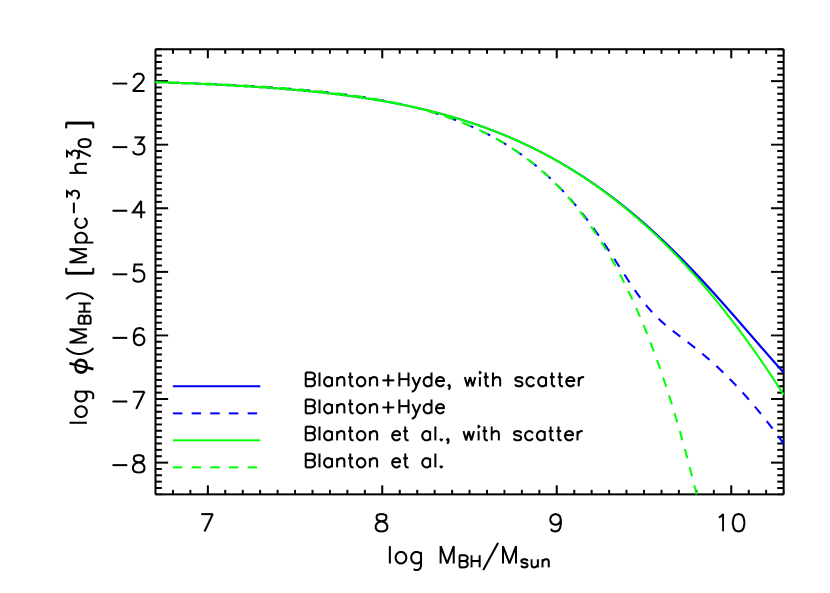
Figure 1.— Distribution of black hole masses predicted by combining the $M_{\bullet}-L$ relation (equation A9) with the SDSS luminosity function and ignoring (dashed) or including (solid) the effect of 0.33 dex scatter around the mean relation. In each case, bottom curve uses the SDSS luminosity function of Blanton et al. (2003), and the top curve uses Blanton et al. augmented with the BCG luminosities of Hyde et al. (2007).

2.3. Effect of scatter in the $M_{\bullet}-L$ relation

To estimate $\phi(M_{\bullet})$ we need both $p(\log M_{\bullet}|L)$ and the distribution of $L$. We use the $r$-band SDSS luminosity function (Blanton et al. 2003) as our basic function, augmented so that it includes a better estimate of the light from the most luminous galaxies.

Briefly, the SDSS photometric pipeline tends to underestimate the luminosities of bright galaxies in crowded fields and of nearby bright galaxies by more than $0.5$ mag (Bernardi et al. 2007a; Lauer et al. 2007; Hyde et al. 2007). The magnitudes of the main galaxy sample are biased low by $\sim 0.1$ mag (see Bernardi 2007 for a discussion of the systematics in the magnitudes and velocity dispersion in the SDSS database and comparisons with the Bernardi et al. 2003a sample). Since these bright galaxies are likely to be massive galaxies, they are likely to host massive black holes, so it is important to correct for this bias. However, doing so is complicated by the fact that the light profiles of these objects are not standard. Hyde et al. (2007) believe that the light profiles are the sum of two components (a galaxy plus inter-cluster light), and only assign the light from the inner component to the object. (Assigning all of the integrated surface brightness to the galaxy makes the discrepancies described below even larger.)

The effect of adding these objects to the luminosity function, and then transforming to a distribution of black hole masses using equation (A9) is shown by the dashed lines in Figure 1. The effect at the luminous end is dramatic: Blanton + Hyde exceeds Blanton alone by many orders of magnitude.

These estimates of black hole abundances ignore the effects of intrinsic scatter in the $M_{\bullet}-L$ relation. The solid curves in Figure 1 show the result of transforming to a distribution of black hole masses using equation (A9) and accounting for scatter of 0.33 dex using equation (3). Including the scatter increases the expected $\phi(M_{\bullet})$ noticably at $M_{\bullet}>10^{8.5}M_{\odot}$; by $M_{\bullet}>10^{9.5}M_{\odot}$ ignoring the scatter results in an underestimate of more than an order of magnitude. In fact, Blanton + scatter exceeds Blanton + Hyde at almost all $M_{\bullet}$. In this respect, accounting for scatter is more important than is getting details of the light profile correct.

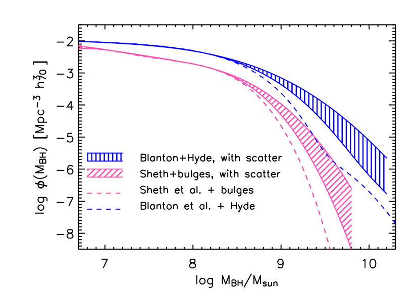
Figure 2.— Luminosity and velocity dispersion-based predictions for the distribution of black hole masses. Curves labeled Sheth et al. were obtained by combining the $\langle M_{\bullet}|\sigma\rangle$ relation of equation (A5) with the observed distribution of velocity dispersions (from Sheth et al. 2003). Curves labeled Blanton+Hyde were obtained by combining the $\langle M_{\bullet}|L\rangle$ relation of equation (A9) with the observed distribution of luminosity from Blanton et al. (2003) and Hyde et al. (2007). The dashed curves assume there is no intrinsic scatter around the $\langle M_{\bullet}|{\rm observable}\rangle$ relations, whereas the hashed regions are bounded by curves in which the intrinsic scatter around the relation was assumed to be $0.22\pm 0.06$ dex for $\langle M_{\bullet}|\sigma\rangle$, and $0.33\pm 0.08$ dex for $\langle M_{\bullet}|L\rangle$ (see Appendix).

2.4. Abundances from the correlation with $\sigma$

Figure 2 shows the results of repeating this analysis, but now with $\langle\log M_{\bullet}|\log\sigma\rangle$ and the distribution of velocity dispersions reported by Sheth et al. (2003). (A word on this choice is necessary, since Bernardi et al. 2006 note that there may be more systems in the SDSS with $\sigma\geq 400$ kms^-1 than the Sheth et al. fitting formula yields. However, HST imaging shows that most of the abnormally large $\sigma$ objects in Bernardi et al. (2006) are objects in superposition; the shape of the Sheth et al. velocity function does not need to be augmented by more systems at $\sigma\geq 400$ kms^-1). For ease of comparison with the luminosity function results shown in the previous subsection, we have used $d\phi(\sigma)/d\sigma$ shown in the final figure of Sheth et al.—this adds an estimate of the contribution of spiral bulges to the measured distribution of early-type galaxy velocity dispersions. Note that this makes essentially no difference at the massive end.

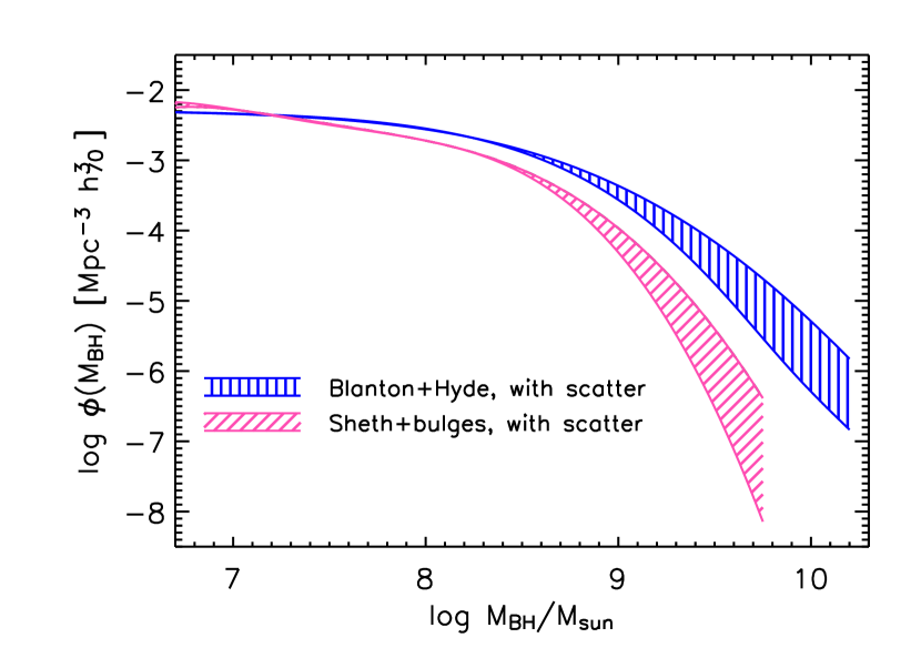
Figure 3.— Accounting for the difference between bulge and total luminosity brings the $L$-based estimate of black hole abundances into better agreement with that based on $\sigma$, although the differences at $M_{\bullet}>10^{9}M_{\odot}$ remain.

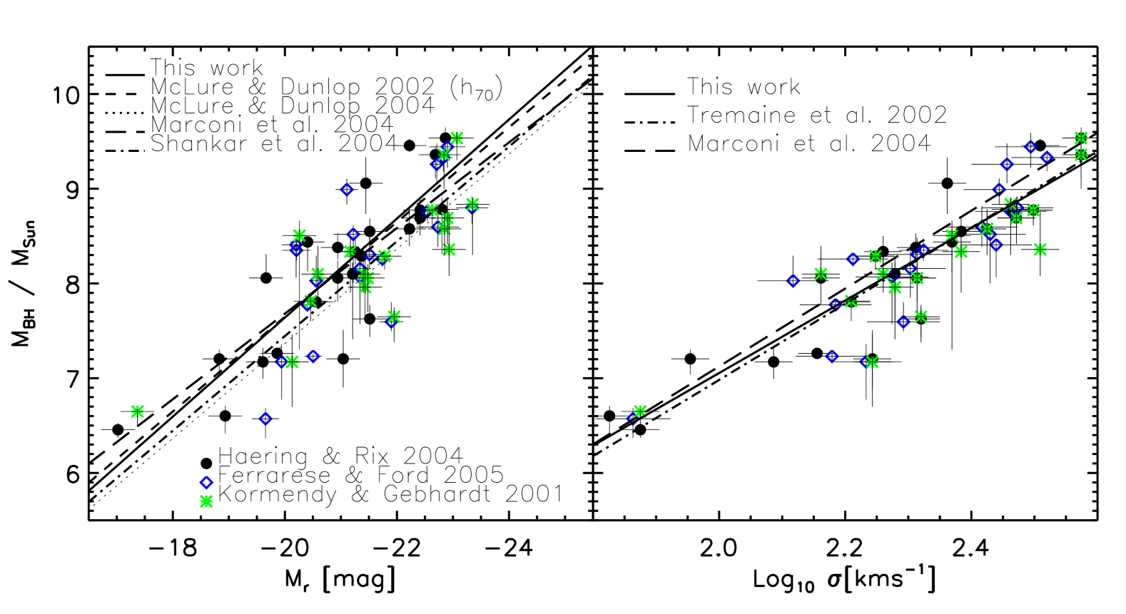
Figure 4.— Left: Correlation between $M_{\bullet}$ and bulge luminosity. Symbols show measurements from a variety of data sets, solid line shows the fit reported in equation (A9), and dashed line shows the fit from McLure & Dunlop (2002) once the difference in Hubble constant has been accounted for. Dotted, dot-dashed and long-dashed lines show the fits used by McLure & Dunlop (2004), Shankar et al. (2004) and Marconi et al. (2004), respectively. In all cases, the fits and data have been shifted to the $r$ band (using $B-r=1.25$, $V-r=0.34$, $r-R=0.27$, $r-I=1.07$ and $r-K=2.7$). Right: Correlation between $M_{\bullet}$ and velocity dispersion. The solid line shows the fit reported in equation (A5). Dot-dashed and long-dashed lines show given in Tremaine et al. (2002) and Marconi et al. (2004), respectively.

The lowest dashed line in the figure shows the expected abundance of supermassive black holes if one ignores the intrinsic scatter in the $\langle\log M_{\bullet}|\log\sigma\rangle$ relation, and the lower hashed region shows the predicted range if this scatter is between 0.16 and 0.28 dex (i.e. $0.22\pm 0.06$ dex, see Appendix). The scatter clearly increases the expected numbers of massive black holes significantly. To appreciate the magnitude of the effect, the upper set of curves show the expected abundances based on Blanton + Hyde combined with the $\langle M_{\bullet}|L_{r}\rangle$ relation of equation (A9) without scatter (upper dashed curve) and with scatter (upper hashed region) between 0.25 to 0.41 dex (i.e. $0.33\pm 0.08$ dex, see Appendix). Notice that the $\sigma$-based prediction when scatter is included is similar to the $L$-based prediction when scatter is ignored.

There is a small inconsistency here which we have investigated but which does not affect our main conclusion. Namely, $L$ in the $M_{\bullet}-L$ relations reported earlier refers to the bulge luminosity. Whereas the bulge accounts for all the luminosity at large $L$, it accounts for a decreasing fraction at lower $L$. We have found that a crude model which sets $L_{\rm bulge}=f(L)\,L$, with $f(L)=(L/L_{*})/(1+L/L_{*})$ yields bulge luminosity densities which are 40% of the total luminosity density in the $g$ and $r$-bands, in good agreement with current estimates. Figure 3 shows the result of incorporating this model for $f(L)$ into our estimates of $\phi(M_{\bullet})$. Doing so brings the $L$- and $\sigma$-based estimates into good agreement at $M_{\bullet}<10^{7.5}M_{\odot}$. However, since $f(L)\to 1$ at large $L$, the large differences at $M_{\bullet}>10^{9}\,M_{\odot}$ remain.

3. Problems and inconsistencies

The smaller intrinsic scatter around $\langle M_{\bullet}|\sigma\rangle$ as compared to $\langle M_{\bullet}|L\rangle$ (equations A5 and A9) suggests that $r_{MV}>r_{ML}$ (equation 2), so $p_{V}(M_{\bullet})$ should predict more massive black holes than $p_{L}(M_{\bullet})$. Figure 2 shows the opposite trend: the estimate based on the Blanton et al. (2003) luminosity function is well in excess of that based on the Sheth et al. (2003) velocity dispersion function. This is true even before adjusting the Blanton et al. function upwards at large $L$ to account for BCGs. This indicates that something has gone wrong with the logic of the previous section.

Furthermore, the analysis of the previous section suggested that, once scatter has been accounted for, both $L$- and $\sigma$-based methods should give the same prediction. Figures 2 and 3 show that the luminosity based predictions are still much larger than those based on velocity dispersion. In this respect, our findings differ markedly from those of McLure & Dunlop (2004), Shankar et al. (2004) and Marconi et al. (2004) who reported that, once scatter had been included, the two estimates agree. As we discuss below, this is because they made different choices for the shape and scatter of the $M_{\bullet}$-observable correlations. Whereas McLure & Dunlop, and Shankar et al. have approximately the same slope as equation (A9), they are shifted to smaller zero-points. Marconi et al. have a shallower slope for $M_{\bullet}-L$, the zero-point of their $M_{\bullet}-\sigma$ is larger, and they make a different choice for the scatter.

3.1. Comparison with previous work

The left hand panel of Figure 4 compares various determinations of $\langle M_{\bullet}|L\rangle$. (In this figure we also show data from Kormendy & Gebhardt (2001) and Ferrarese & Ford (2005)—although we only use their measurements of the objects which are in common with Häring & Rix (see Appendix A in Bernardi et al. 2007b for a decription of how the black hole sample was compiled). We use these other measurements primarily to demonstrate the uncertainties on the measurements—all the fits we show and use come only from the Häring & Rix data.)

Both the McLure & Dunlop (2004) and Shankar et al. (2004) results are based on the determination of $M_{\bullet}-L$ by McLure & Dunlop (2002): $\log M_{\bullet}=-0.5M_{\rm R}-2.91$. McLure & Dunlop (2002) say that this determination assumes $H_{0}=50$ km s^-1 Mpc^-1. Shankar et al. (2004) say that the result of shifting this relation to $H_{0}=70$ km s^-1 Mpc^-1 is to change the zero point from $-2.91$ to $-2.69$. This results from rescaling both the luminosities and the black hole masses: the net shift is $1.25\log(70/50)^{2}-\log(70/50)=0.22$, the first term coming from shifting the luminosities, and the second from the masses. Note that this rescaling would be appropriate if both $M_{\bullet}$ and $L$ in the 2002 paper assumed the same $H_{0}$, but would be inappropriate if not.

Shankar et al.’s (2004) shift differs slightly from that of McLure & Dunlop (2004) who state that, if $H_{0}=70$ km s^-1 Mpc^-1 and $R-K=2.7$, then their fit from 2002 implies $\log M_{\bullet}=1.25\,\log L_{\rm K}/L_{\odot{\rm K}}-5.76$. Now, $M_{\odot{\rm K}}=3.28$, so the right hand side of this relation is $-0.5\,(M_{\rm R}-2.7-3.28)-5.76=-0.5\,M_{\rm R}-2.77$. This relation predicts $M_{\bullet}$ that are lower by 0.08 dex than does the relation used by Shankar et al. (2004). The source of this discrepancy is unclear, but it is a curious coincidence that $\log(70/50)=0.146$ is close to the $2.91-2.77$ shift that McLure & Dunlop require: this would be the shift if $M_{\bullet}\propto L_{\rm R}$ rather than $\propto L_{\rm R}^{1.25}$.

Figure 5.— Black hole abundances associated with some of the $M_{\bullet}-L$ relations shown in the previous figure. All curves assume the $r$-band luminosity function from Blanton et al. (2003) except for Marconi et al. (2004) which is based on the early-type galaxy sample of Bernardi et al. (2003a). Clearly, the fit which produces larger black hole masses for a given luminosity results in the most supermassive black holes. The hashed region labeled Sheth et al. were obtained by combining the $\langle M_{\bullet}|\sigma\rangle$ relation of equation (A5) with the observed distribution of velocity dispersions (from Sheth et al. 2003). This region is bounded by curves in which the intrinsic scatter around the relation $\langle M_{\bullet}|\sigma\rangle$ was assumed to be 0.16 and 0.28 dex.

The McLure & Dunlop (2004) and Shankar et al. (2004) relations are shown as the dotted and dot-dashed lines in Figure 4. Both have been shifted from $R$ to $r$ using $r-R=0.27$, and both lie below the Häring & Rix data. To study why, we returned to the issue of whether or not both $L$ and $M_{\bullet}$ should have been rescaled when $H_{0}$ was changed. McLure & Dunlop (2002) report that their $M_{\bullet}-\sigma$ relation is essentially the same as that of Tremaine et al. (2002). Therefore, they must be using the same $M_{\bullet}$ values as Tremaine et al. However, the Tremaine et al. analysis actually assumes $H_{0}=80$ km s^-1 Mpc^-1 rather than 50 km s^-1 Mpc^-1. To illustrate the effect this has, suppose we rescale the $M_{\bullet}$ values in their 2002 fit by (70/80), and the $R$-band luminosities by $(70/50)^{2}$. This would make their relation $\log M_{\bullet}=-0.5M_{\rm R}-2.91+2.5\log(70/50)-\log(70/80)=-0.5M_{\rm R}-2.49$; this is a shift in zero point of 0.42. Shifting this from $R$ to $r$ using $r-R=0.27$ as before yields the short dashed line. It is in substantially better agreement with the Häring & Rix data than is the dotted line.

The relations used by McLure & Dunlop and Shankar et al. clearly produce smaller black holes for a given luminosity. The most important effect of this is to decrease the $L-$based estimate of the number of objects with $M_{\bullet}>10^{9}M_{\odot}$. This is shown in Figure 5. The dotted, dashed and dot-dashed curves show the result of inserting the McLure & Dunlop (2002-2004) and Shankar et al. (2004) based $\langle M_{\bullet}|L\rangle$ relations in equation (3), respectively, when the scatter is assumed to be 0.33 dex. The solid line shows $\phi(M_{\bullet})$ for our fit, and the hashed region shows the $\sigma-$based abundances. Clearly, the $\langle M_{\bullet}|L\rangle$ relation with the smallest zero-point, that of McLure & Dunlop (2004), produces the fewest massive black holes. McLure & Dunlop are able to account for the small difference which remains between the $L$ and $\sigma$-based estimate by assigning a larger scatter to the $M_{\bullet}-\sigma$ relation, 0.3 dex, rather than the 0.22 dex which we used to produce Figure 5. However, the left hand panel in Figure 4 suggests that the lower zero-point is unacceptably low, and 0.3 dex is larger than all recent estimates of the scatter around $\langle M_{\bullet}|\sigma\rangle$.

Marconi et al. (2004) also found consistency between the two estimates. They believe that this is because the scatter in the $M_{\bullet}-L$ and $M_{\bullet}-\sigma$ relations are similar (they believe both are about 0.3 dex). We believe that it is their choice of relations combined with the scatter around the relations which is the cause of the agreement (the analysis of the previous section shows clearly that having equal scatter in the two relations is neither sufficient nor necessary). To illustrate, the long dashed line in Figure 5 shows the $M_{\bullet}$ distribution computed by Marconi et al. (2004) from the $L$-based approach (at lower $M_{\bullet}$ it differs from the other works mainly because Marconi et al. used the early-type galaxy luminosity function from Bernardi et al. 2003b instead of the luminosity function of all types from Blanton et al. 2003). Their $\sigma$-based approach gives a similar curve provided one uses their $M_{\bullet}-\sigma$ relation, shown as the long dashed line in the right panel of Figure 4, with intrinsic scatter of $0.3$ dex. The hashed region labeled Sheth et al. was obtained by combining the $\langle M_{\bullet}|\sigma\rangle$ relation of equation (A5) with the observed distribution of velocity dispersions (from Sheth et al. 2003). This region is bounded by curves in which the intrinsic scatter around the relation $\langle M_{\bullet}|\sigma\rangle$ was assumed to be 0.16 and 0.28 dex (note that the larger limit is similar to the value used by Marconi et al., i.e. 0.3 dex). However, in this case the $L$ (long dashed line) and $\sigma$ (upper bound of hashed region) based estimates are different. Marconi et al. found consistency between the two estimates because the $M_{\bullet}-\sigma$ relation they used is steeper and shifted to larger $M_{\bullet}$ values than our relation (see right hand panel of Figure 4), so their $\sigma$s produce larger $M_{\bullet}$s.

Although Marconi et al. (2004), McLure & Dunlop (2004), and Shankar et al. (2004) were able to obtain $L$-based estimates of $\phi(M_{\bullet})$ which were in good agreement with those based on $\sigma$, the analysis above suggests that this was largely due to a fortuitous inconsistency resulting from how one rescales $M_{\bullet}$ and $L$ when changing the Hubble constant. However, in the next subsection we discuss why, if the Hubble-constant related scalings are all done self-consistently, then the $\sigma-$ and $L-$based estimates should not have given the same answer!

3.2. The $\sigma-L$ relation

Why do our $L-$ and $\sigma-$based estimates give different answers? If we transform the SDSS-B07 luminosity distribution into one for $\sigma$ using equations (A10) and (3), and then to a distribution of $M_{\bullet}$ using equations (A5) and (3), then this gives the same answer as transforming SDSS-B07 luminosity into $M_{\bullet}$ directly using equations (A9) and (3). This is exactly as expected from the toy model described in the previous section. However the intermediate step provides a predicted velocity function which disagrees with the SDSS-B07 one (from Sheth et al. 2003). Figure 6 shows this explicitly; the hashed region shows the result of starting with the SDSS $\phi(L)$ and using the black hole $\langle\sigma|L\rangle$ relation and scatter (equation (A10)) to infer $\phi(\sigma)$. The range of values comes from including the uncertainty in the slope and scatter of $\langle\sigma|L\rangle$. The disagreement with the actual measured $\phi(\sigma)$ distribution (solid curve) strongly suggests that the $\sigma-L$ relation in the black hole samples is not the same as in the SDSS-B07 sample, and that this is the source of the discrepancy between the $L-$ and $\sigma-$based estimates.

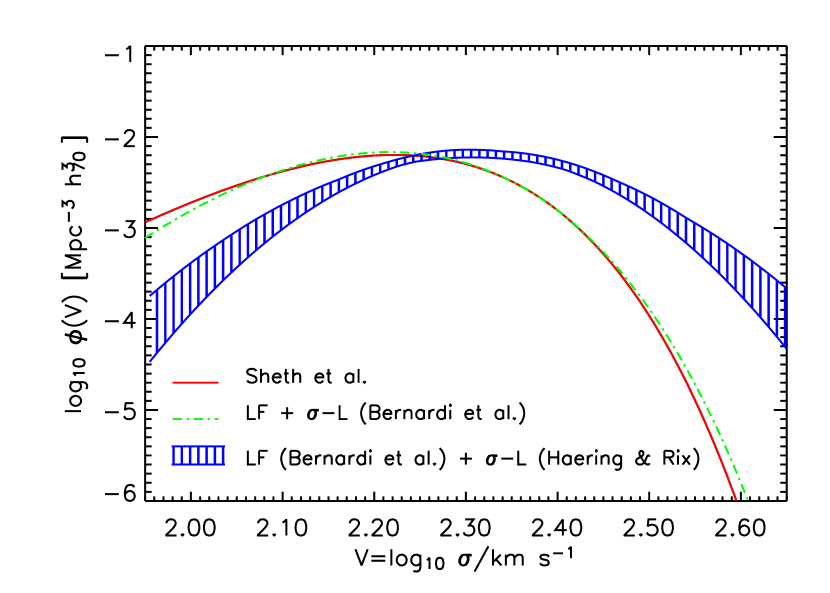
Figure 6.— Observed and predicted distribution of $\sigma$; solid curve shows the velocity function reported by Sheth et al. (2003); dot-dashed line shows the result of starting from the luminosity function of Bernardi et al. (2003b), and using the SDSS $\langle\sigma|L\rangle$ relation and its scatter to infer $\phi(\sigma)$, whereas hashed region uses the $\langle\sigma|L\rangle$ relation and scatter from the black hole sample of Häring & Rix (2004) instead. The $\langle\sigma|L\rangle$ relation for the black hole sample is rather uncertain, since it is derived from only $\sim 30$ objects: the hashed region shows the range of predicted $\phi(\sigma)$ associated with allowing the slope and scatter of the $\sigma-L$ relation to vary within one standard deviation of their rms values.

In SDSS-B07,

$$\Bigl{\langle}\log\sigma|M_{r}\Bigr{\rangle}_{\rm SDSS-B07}=2.287-{0.255\over 2.5}\,(M_{r}+22),$$ (4)

with an error in the slope and zero-point of $0.009$ and $0.005$, respectively, whereas it is

$$\Bigl{\langle}\log\sigma|M_{r}\Bigr{\rangle}=2.42-{0.34\over 2.5}\,(M_{r}+22)$$ (5)

in the Häring & Rix sample (equation A10). The errors in the slope and zero-point are $0.02$ and $0.01$, respectively. Note that this slope of $-0.34/2.5=-0.14$ is rather different from the canonical value of $-0.10$: At a given luminosity, the black hole samples have $\log\sigma$ larger by about 0.08 dex than the SDSS-B07—observational errors are typically only about $0.03$ dex.

Yu & Tremaine (2002) also considered the possibility that the $\sigma-L$ relation was the cause of the discrepancy, and suggested that perhaps there are systematic differences between SDSS-B07 velocity dispersions and those derived from more local samples. A direct test of this possibility is difficult because, of the $\sim 30$ objects in the Häring & Rix compilation, only about ten have SDSS imaging, and only NCG 4261 has an SDSS spectrum as well. For the objects in common, the SDSS apparent magnitudes are about 0.5 mags fainter than those used in the black hole analyses, but this is almost certainly due to the sky subtraction problems for bright objects to which we refered earlier (Hyde et al. 2007). In any case, correcting for this will increase the SDSS luminosities, further exacerbating the discrepancy in the $\sigma-L$ relation.

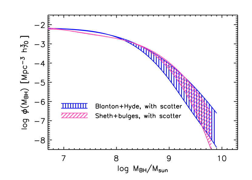
Figure 7.— Predicted abundances if the luminosities of the black hole hosts are modified so that they define a $\langle\sigma|L\rangle$ relation which has the same slope and zero-point as the SDSS-B07 relation. This rescaling modifies the $\langle M_{\bullet}|L\rangle$ relation, but leaves the $\langle M_{\bullet}|\sigma\rangle$ relation unchanged. As a result the curve labeled ‘Sheth + bulges’ is the same as before, but ‘Blanton + Hyde’ now produces many fewer massive objects.

A detailed discussion of the $\sigma-L$ relation computed from different samples, analysis of systematic biases which affect the samples, and the effect of correcting “naively” the nearby samples for peculiar velocities, is presented in Bernardi (2007). Compared to any of these early-type galaxy samples, the $\sigma-L$ relation in black hole samples is biased to larger $\sigma$ for given $L$, or to smaller $L$ for a given $\sigma$ (Bernardi et al. 2007b). In view of this discrepancy, whatever the cause, the fact that McLure & Dunlop (2004), Marconi et al. (2004) and Shankar et al. (2004) obtained consistent estimates of $\phi(M_{\bullet})$ from both $L$ and $\sigma$ is remarkable indeed.

Figure 7 shows the result of assuming that the velocity dispersion estimates in the black hole sample are reliable, but the distances, and so the luminosities, are not. It was constructed by rescaling all the bulge luminosities of the black hole hosts so that they define a relation with the same slope as in equation (4), though with different scatter. To do so, we added $-0.978+0.25\,(Mr+22)$ to each of the absolute magnitudes in the black hole sample, as suggested by the difference between equations (4) and (5).

These rescaled luminosities were used to estimate a new $\langle M_{\bullet}|L_{r}\rangle$ relation, which was then inserted in equation (3) to predict black hole abundances from the luminosity function. The resulting abundances are considerably lower, because the rescaled luminosities define a considerably shallower $\langle M_{\bullet}|L_{r}\rangle$ relation, meaning that considerably larger $L$ is required to reach $M_{\bullet}>10^{9}M_{\odot}$. While this rescaling is probably unrealistic, we have included the result to illustrate the importance of the $\sigma-L$ relation when comparisons of the $L-$ and $\sigma-$based estimates of $\phi(M_{\bullet})$ are made. A more careful accounting of the role of selection effects is presented in Bernardi et al. (2007b).

4. Discussion

It is common to estimate the abundance of supermassive black holes by combining observed correlations between $M_{\bullet}$ and bulge luminosity or velocity dispersion, calibrated from relatively small samples, with luminosity or velocity dispersion functions determined from larger samples. However, the $\langle M_{\bullet}|\sigma\rangle$ and $\langle M_{\bullet}|L\rangle$ relations have intrinsic scatter of about 0.22 and 0.33 dex (Appendix). Accounting for this results in considerably increased estimates of the abundance of black holes with $M_{\bullet}\geq 10^{9}\,M_{\odot}$, compared to naive estimates which ignore this scatter. Doing so is at least as important as correcting the luminosity function for the fact that the most luminous galaxies have non-standard light profiles (Figure 1). Once this scatter has been accounted for, the $\sigma$-based estimates of $\phi(M_{\bullet})$ are in reasonably good agreement with models, such as that of Hopkins et al. (2006), which relate previous QSO and AGN activity to the local black hole mass function. The luminosity-based estimates, on the other hand, are substantially in excess of this model.

These results follow from using a single power-law to parametrize the $M_{\bullet}-\sigma$ and $M_{\bullet}-L$ relations. While this may be too simplistic, this parametrization is not the primary reason why the $L-$ and $\sigma-$based approaches yield different predictions for black hole abundances. The main cause of the discrepancy is that the $\sigma-L$ correlation in black hole samples is different from that in the samples from which the luminosity and velocity functions are drawn: the black hole samples have larger $\sigma$ for a given $L$ compared to the ENEAR or SDSS-B07 samples or have smaller $L$ for a given $\sigma$ (Bernardi et al. 2007b). If this is a physical effect, then it compromises the fundamental assumption of black hole demographic studies—that all galaxies host black holes. If, on the other hand, it is a selection effect, then the $M_{\bullet}-\sigma$ and $M_{\bullet}-L$ relations currently in the literature are biased compared to the true relations, making current estimates of black hole abundances unreliable. If black hole masses correlate with bulge luminosity only because of the $M_{\bullet}-\sigma$ and $\sigma-L$ relations, then the bias in the $\sigma-L$ relation is not important only if one is using $\phi(\sigma)$ to infer black hole abundances: the $\phi(L)$-based estimate may be strongly affected.

Identifying the source of the bias is complicated. Residuals from the size-luminosity relation are anti-correlated with residuals from the $\sigma-L$ relation, as might be expected from the virial theorem (Bernardi et al. 2003b). If the stellar kinematics method of measuring black hole masses favors objects with high surface brightnesses, then one might expect smaller sizes and larger $\sigma$ at constant $L$: this would produce a bias in the sense we see. On the other hand, it might be more difficult to measure the influence of the black hole on stellar kinematics if the stellar velocity dispersion is already abnormally large—this would produce a bias in the opposite sense. Whether either or these effects has played a role in the selection of black samples is an open question. See Bernardi et al. (2007b) for further study along these lines.

This Appendix describes our procedure for estimating the slope and scatter associated with $\langle M_{\bullet}|O\rangle$. Let $y=\log M_{\bullet}-\langle\log M_{\bullet}\rangle$, and $x=O-\langle O\rangle$, and let $\sigma_{x}$, $\sigma_{y}$ and $r_{xy}$ denote the true intrinsic rms values of $x$, $y$, and the cross-correlation coefficient. Finally, let $\epsilon_{x}$ and $\epsilon_{y}$ denote the typical measurement errors in determining $x$ and $y$. In practice, the estimated error may vary from object to object; in using a single representative value, our analysis below ignores this additional information. Minimizing

$$\chi^{2}\equiv\sum_{i=1}^{N}(y_{i}-ax_{i}-b)^{2}/N$$ (1)

with respect to $a$ and $b$ yields

$$a_{\rm min}={\sum_{i}x_{i}y_{i}\over\sum_{i}x_{i}^{2}}={\sigma_{x}\sigma_{y}r_{xy}\over\sigma_{x}^{2}+\epsilon_{x}^{2}}={\sigma_{x}\sigma_{y}r_{xy}\over\sigma_{x}^{2}}\left(1+{\epsilon_{x}^{2}\over\sigma_{x}^{2}}\right)^{-1}=a_{y|x}\,\left(1+{\epsilon_{x}^{2}\over\sigma_{x}^{2}}\right)^{-1}$$ (2)

and, because both $x$ and $y$ have zero mean, $b_{\rm min}=0$. Comparison with equation (1) shows that $a_{\rm min}$ differs from the true slope $a_{y|x}$ because of the measurement errors $\epsilon_{x}^{2}$. (We have assumed uncorrelated measurement errors in $x$ and $y$. Hence, these errors affect the mean of $x^{2}$, and of $y^{2}$, but not the correlation between $x$ and $y$.) The scatter around this relation is

$$\chi^{2}_{\rm min}=\sigma_{x}^{2}\,(1-r_{xy}^{2})+\epsilon_{y}^{2}+a_{\rm min}^{2}\,\epsilon_{x}^{2}\left(1+{\epsilon_{x}^{2}\over\sigma_{x}^{2}}\right).$$ (3)

The uncertainty on the value of this minimum is $\chi^{2}_{\rm min}\sqrt{2(N-1)/N^{2}}$: for $N=24$ the estimated scatter is uncertain by about $\sqrt{46}/24\sim$ thirty percent.

Comparison with equation (2) shows that the first term in the expression above represents the intrinsic scatter around the true relation, and the other terms are a consequence of the measurement errors. Hence, the intrinsic slope and scatter which we report in the main text are

$$a_{\rm y|x}=a_{\rm min}\,\left(1+{\epsilon_{x}^{2}\over\sigma_{x}^{2}}\right)\qquad{\rm and}\qquad\sigma^{2}_{\rm y|x}=\chi^{2}_{\rm min}-\epsilon_{y}^{2}-a_{\rm min}^{2}\,\epsilon_{x}^{2}\left(1+{\epsilon_{x}^{2}\over\sigma_{x}^{2}}\right).$$ (4)

Notice that $a_{y|x}$ can be determined well even if $\epsilon_{y}$ is large; of course large uncertainties in $y$ do affect the scatter around the mean relation. There will be trouble only if $\sigma_{x}\ll\epsilon_{x}$; in this case, the large measurement errors in $x$ have largely erased the correlation between $x$ and $y$, so a small measured slope requires a large correction factor to restore it to the true value.

We have applied this procedure to the dataset of Häring & Rix (2004), who provide estimates of $M_{\bullet}$, $\sigma$, $M_{\rm bulge}$ and $L_{r}$ and the fraction of this luminosity which is from the bulge (Appendix A in Bernardi et al. 2007b describes exactly how the black hole sample was compiled and the conversion from B, V, R and I-band luminosities to SDSS $r-$band. Both luminosities and the black hole masses were scaled to $H_{0}=70$ km s^-1 Mpc^-1). When doing so we will deal almost exclusively with logarithmic quantities; when taking the logarithm, $M_{\bullet}$ is in units of $M_{\odot}$, $\sigma$ is in kms^-1, and the associated measurement errors are $\epsilon_{\log M_{\bullet}}\sim 0.2$ dex, $\epsilon_{\log\sigma}\sim 0.03$ dex, and $\epsilon_{\log M_{\rm bulge}}\sim 0.18$ dex. The scatter around the correlations we report are estimates of the intrinsic scatter. The uncertainties in the slope, zero-point, and scatter of the following relations were computed by bootstrap resampling. Application of the procedure outlined above yields

$$\Bigl{\langle}\log M_{\bullet}|\log\sigma\Bigr{\rangle}=(8.21\pm 0.06)+(3.83\pm 0.21)\,\log\left({\sigma\over 200\,{\rm kms}^{-1}}\right)$$ (5)

with intrinsic scatter of $0.22\pm 0.06$ dex, and

$$\Bigl{\langle}\log M_{\bullet}|\log M_{\rm bulge}\Bigr{\rangle}=(8.31\pm 0.10)+(1.06\pm 0.12)\,\log\left({M_{\rm bulge}\over 10^{11}M_{\odot}}\right)$$ (6)

with rms scatter $0.33\pm 0.08$ dex. Bulge mass and luminosity are tightly correlated (Häring & Rix 2004):

$$\Bigl{\langle}\log M_{\rm bulge}|M_{r}\Bigr{\rangle}=11.35-0.492\,(M_{r}+22)$$ (7)

with negligible scatter, so inserting this fit in the previous one yields

$$\Bigl{\langle}\log M_{\bullet}|M_{r}\Bigr{\rangle}=8.69-{1.31\over 2.5}\,(M_{r}+22)$$ (8)

with scatter of $0.33$ dex. As a check, we have also fit for the correlation between $M_{\bullet}$ and $M_{r}$ directly, finding

$$\Bigl{\langle}\log M_{\bullet}|M_{r}\Bigr{\rangle}=(8.68\pm 0.10)-{(1.30\pm 0.15)\over 2.5}\,(M_{r}+22)$$ (9)

with scatter of $0.34\pm 0.09$ dex. The main text also considered the correlation between $L$ and $\sigma$ in this data set. It is

$$\Bigl{\langle}\log\sigma|M_{r}\Bigr{\rangle}=(2.42\pm 0.01)-{(0.34\pm 0.02)\over 2.5}\,(M_{r}+22)$$ (10)

with scatter of $0.04\pm 0.01$ dex. Note that this slope is rather different from the canonical value of $-0.10$.

References

- (1) Aller, M. C., & Richstone, D. 2002, AJ, 124, 3035
- (2) Bernardi, M., Sheth, R. K., Annis J. et al. 2003a, AJ, 125, 1817
- (3) Bernardi, M., Sheth, R. K., Annis J. et al. 2003b, AJ, 125, 1849
- (4) Bernardi, M., Sheth, R. K., Nichol, R. C. et al. 2005, AJ, 129, 61
- (5) Bernardi, M., Sheth, R. K., Nichol, R. C. et al. 2006, AJ, 131, 2018
- (6) Bernardi, M., Hyde, J. B., Sheth, R. K., Miller, C. J., Nichol, R. C. 2007a, AJ, in press (astro-ph/0607117)
- (7) Bernardi, M., Sheth, R. K., Tundo, E., Hyde J. B. 2007b, ApJ, in press (astro-ph/0609300)
- (8) Bernardi, M. 2007, AJ, in press (astro-ph/0609301)
- (9) Blanton, M., R., et al. 2003, ApJ, 592, 819
- (10) Cattaneo, A., & Bernardi, M. 2003, MNRAS, 344, 45
- (11) Cavaliere, A., & Vittorini, V. 2002, ApJ, 570, 114
- (12) da Costa, L. N., Bernardi, M., Alonso, M. V., Wegner, G., Willmer, C. N. A., Pellegrini, P. S., Ritè, C., & Maia, M. A. G. 2000, AJ, 120, 95
- (13) Ferrarese, L., & Merritt, D. 2000, ApJ, 539, L9
- (14) Ferrarese, L., Ford, H. 2005, Space Science Reviews, 116, 523
- (15) Gebhardt, K., et al. 2000, ApJ, 539, L13
- (16) Granato, G. L., Silva, L., Monaco, P., Panuzzo, P., Salucci, P., De Zotti, G., & Danese, L. 2001, MNRAS, 324, 757
- (17) Haiman, Z., Ciotti, L., Ostriker, J. P. 2004, ApJ, 606, 763
- (18) Haiman, Z., Jimenez, R., & Bernardi, M. 2006, ApJ, submitted
- (19) Häring, N., & Rix, H. 2004, ApJ, 604, 89L
- (20) Hyde, J. B., Bernardi, M., Sheth, R. K. et al. 2007, AJ, submitted
- (21) Hopkins, P. F., Hernquist, L., Cox, T. J., Di Matteo, T., Robertson, B., & Springel, V. 2006, ApJS163, 1
- (22) Kauffmann, G. & Haehnelt, M. 2000, MNRAS, 311, 576
- (23) Kormendy J., Gebhardt, K., 2001, in Wheeler J. C., Martel H. eds, AJP Conf. Proc. 586, 20th Texas Symposium on Relativistic Astrophysics. Am. Inst. Phys., Melville, p.363
- (24) Lapi, A., et al. 2006, ApJ, submitted (astro-ph/0603819)
- (25) Lauer, T. R., et al. 2007, ApJ, submitted (astro-ph/0606739)
- (26) Marconi, A., & Hunt, L. K. 2003, ApJ, 589, L21
- (27) Marconi, A., Risaliti, G., Gilli, R., Hunt, L. K., Maiolino, R., & Salvati, M. 2004, MNRAS, 351, 169
- (28) McLure, R. J., & Dunlop, J. S. 2002, MNRAS, 331, 795
- (29) McLure, R. J., & Dunlop, J. S. 2004, MNRAS, 352, 1390
- (30) Monaco, P., Salucci, P., & Danese, L. 2000, MNRAS, 311, 279
- (31) Novak, G., Faber, S. M., Dekel, A. 2006, ApJ, 637, 96
- (32) Prugniel, Ph., & Simien, F. 1996, A&A, 309, 749
- (33) Shankar, F., Salucci, P., Granato, G. L., De Zotti, G., and Danese, L. 2004, MNRAS, 354, 1020
- (34) Sheth, R. K., Bernardi, M., Schechter, P. L., et al. 2003, ApJ, 594, 225
- (35) Tremaine, S., et al. 2002, ApJ, 574, 740
- (36) Yu, Q., & Lu, Y. 2004, ApJ, 602, 603
- (37) Yu, Q., & Tremaine, S. 2002, MNRAS, 335, 965