On the ultra-high energy
cosmic ray horizon

Abstract

We compute the ultra-high energy cosmic ray horizon, i.e. the distance up to which cosmic ray sources may significantly contribute to the fluxes above a certain threshold on the observed energies. We obtain results both for proton and heavy nuclei sources.

1 Introduction

Soon after the discovery of the cosmic microwave background (CMB) radiation it was realized by Greisen, Zatsepin and Kuzmin [1] that the fluxes of cosmic ray (CR) protons with energies of order $10^{20}$ eV and above would be strongly attenuated over distances of few tens of Mpc. This is due to the energy losses caused by the photo-pion production processes in the interactions of the protons with the CMB photons. Similarly, if CR sources accelerate heavy nuclei, these can photodisintegrate into lighter ones as they interact with CMB and infrared (IR) photons on their journey to us. In this way the fragments may arrive to the Earth with significantly smaller energies than the parent nuclei produced at the sources. Moreover, both protons and heavy nuclei can further loose energy by pair production processes, although due to the small inelasticities involved the typical attenuation length associated to $e^{+}e^{-}$ production at ultra-high energies is large ($\sim 1$ Gpc for protons).

Many works have studied these processes (see e.g. refs. [2, 3, 4, 5, 6, 7, 8, 9, 10, 11] for the case of protons, and [12, 13, 14, 15, 16, 17, 18] for nuclei), and our purpose here is to make a detailed analysis to present the results in a way which can be useful for the study of correlations between the arrival directions of the highest energy cosmic rays (we will focus here on energies above 50 EeV, where 1 ${\rm EeV}\equiv 10^{18}$ eV) and candidate astronomical sources. Assuming that the sources are distributed uniformly and have similar absolute cosmic ray luminosities, we will obtain the distances within which the major part of the observed events should be produced (i.e. the horizon for the potential sources) as a function of the threshold adopted for the energies of the events.

2 The horizon for protons

The attenuation length $\lambda$ for the propagation of protons is just

$$\lambda^{-1}\equiv-\frac{1}{E}\frac{{\rm d}E}{{\rm d}x}=\lambda_{\gamma\pi}^{-1}+\lambda_{ee}^{-1}+\lambda_{z}^{-1},$$ (1)

receiving contributions from photo-pion ($\lambda_{\gamma\pi}$), pair creation ($\lambda_{ee}$) and redshift ($\lambda_{z}$) losses.

The attenuation length from photo-pion production by the protons in interaction with the CMB photons is given by (we use hereafter natural units)

$$\lambda_{\gamma\pi}^{-1} = \frac{1}{2\gamma^{2}}\int_{0}^{\infty}\frac{{\rm d}\epsilon}{\epsilon^{2}}\frac{{\rm d}n}{{\rm d}\epsilon}\int_{0}^{2\gamma\epsilon}{\rm d}\epsilon^{\prime}\ \epsilon^{\prime}\eta(\epsilon^{\prime})\sigma(\epsilon^{\prime})$$ (2)

$$= -\frac{kT}{2\pi^{2}\gamma^{2}}\int_{0}^{\infty}{\rm d}\epsilon^{\prime}\ \epsilon^{\prime}\eta(\epsilon^{\prime})\sigma(\epsilon^{\prime})\;{\rm ln}\left[1-\exp(-\epsilon^{\prime}/2\gamma kT)\right],$$ (3)

where $\gamma=E/m_{p}$ is the Lorentz factor and the CMB photon density in the observer’s rest frame is

$$\frac{{\rm d}n}{{\rm d}\epsilon}=\frac{\epsilon^{2}}{\pi^{2}\left(\exp(\epsilon/kT)-1\right)},$$ (4)

being characterized by a temperature $T=2.73^{\circ}$K. The cross section for pion production in terms of the photon energy $\epsilon^{\prime}$ in the proton’s rest frame is $\sigma(\epsilon^{\prime})$ and the inelasticity factor $\eta(\epsilon^{\prime})$ is the average fraction of the proton energy lost in the process. We use for the product $\sigma\eta$ a fit to the average values given in [8], which includes both single pion production near the $\Delta$ resonance and multi-pion production at higher energies.

This attenuation length, as well as that due to pair production obtained following [19, 20], are depicted in fig. 1 as a function of the proton energy. The redshift losses, characterized by $\lambda_{z}\sim c/H_{0}\simeq 4$ Gpc, are of no relevance for the energies considered in the present work, for which the effects due to the interactions with the photon background are the dominant ones.

Figure 1: Proton attenuation length vs. energy.

A direct way to compute the CR horizon is to follow the trajectories of many individual protons with initial energies distributed according to a given input spectrum, here taken as a power law one, d$N/{\rm d}E\propto E^{-\alpha}$ (we will show results for $\alpha=2.2$ and 2.7). We then obtain the attenuation factor $A(E_{th},x)$, which is defined as the fraction of the particles which originally had an energy above a threshold value $E_{th}$ that still have an energy above that threshold after traversing a distance $x$. Assuming that the sources are uniformly distributed and have similar intrinsic CR luminosities and spectra, one finds that the fraction of the events observed above a given energy threshold which originated in sources farther than a distance $D$ is just

$$F(E_{th},D)={\int_{D}^{\infty}{\rm d}x\ A(E_{th},x)\over\int_{0}^{\infty}{\rm d}x\ A(E_{th},x)}.$$ (5)

Since we will be interested in threshold energies above 50 EeV, cosmological effects due to the Universe’s expansion or to source evolution are negligible. This implies that the effects of the inverse square distance reduction of the fluxes from each source and the increase in the number of sources with distance compensate each other, leaving just the simple integrals in eq. (5).

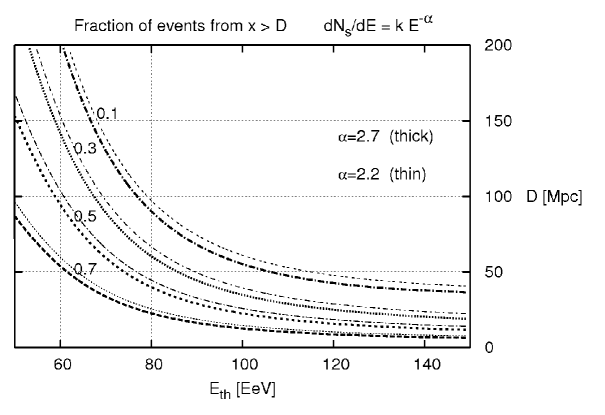
Figure 2: Considering the events arriving with energies above $E_{th}$, the contours indicate the fraction originating from distances larger than $D$, assuming a uniform distribution of proton sources with similar intensity.

The fraction $F$ is depicted in fig. 2. We see that the horizon for protons, which may be taken as the distance for which this fraction reaches e.g. 10%, is relatively close on cosmological grounds for all the energies considered. For instance, for $E_{th}=80$ EeV one has that 90% of the events should have been produced at distances not farther than $\sim 90$ Mpc. The sensitivity to the assumed source spectral index $\alpha$ is not large, although as expected the horizon increases for harder spectra since above a given threshold the fraction of higher energy events, which are more penetrating, becomes larger in this case. Let us also mention that the pair production losses have an impact on the results only for $E_{th}<80$ EeV, and they become indeed quite important for $E_{th}<60$ EeV.

Note that since for a power law spectrum the number of events above a given threshold is proportional to $E_{th}^{-\alpha+1}$, one has simply that $A(E_{th},x)=\left(E_{th}/E^{\prime}_{th}(x)\right)^{\alpha-1}$, where $E^{\prime}_{th}(x)$ is the initial energy that a CR proton should have in order to arrive with an average energy $E_{th}$ after traversing a distance $x$. The energies $E^{\prime}_{th}$ can be easily computed by solving the evolution equation, d$E/{\rm d}x=-E/\lambda$, backwards in time. We checked that this simpler procedure leads indeed to the same results as the Monte Carlo computations discussed before, but it has the drawback that it cannot be generalized to the case of heavy nuclei, since for these last it is not possible to know in advance the final average mass of the fragment after the nucleus has propagated a given distance.

Let us mention that we are using the so-called continuous energy loss approximation to evolve the CR energies. This does not account for the fluctuations originating from the stochastic nature of the pion production processes. Although these fluctuations could be relevant for the study of detailed features in the differential CR spectrum (such as the ‘bump’ preceding the GZK cutoff), they have only a minor impact on the quantities we compute, which are based on the integral spectra above specified thresholds.

3 The horizon for nuclei

Figure 3: Attenuation lengths vs. energy for different nuclei. Lower curves are due to photo-disintegration processes and upper curves to pair production processes.

The rate at which a nucleus of mass number $A$ photo-disintegrates with the emission of $i$ nucleons is given by

$$R_{A,i}=\frac{1}{2\gamma^{2}}\int_{0}^{\infty}\frac{{\rm d}\epsilon}{\epsilon^{2}}\frac{{\rm d}n}{{\rm d}\epsilon}\int_{0}^{2\gamma\epsilon}{\rm d}\epsilon^{\prime}\ \epsilon^{\prime}\sigma_{A,i}(\epsilon^{\prime}),$$ (6)

where now $\gamma=E/Am_{p}$. The relevant photon densities in this case are the CMB and the IR backgrounds. For this last we use the estimates obtained in [21]. The cross sections $\sigma_{A,i}$ for the different processes in which a nucleus of mass number $A$ emits $i$ nucleons were parametrised in [12], and we also use the updated energy threshold values presented in [14]. To describe the average energy loss of a given nucleus it is convenient to introduce the effective rate [12]

$$R_{A,eff}\equiv\sum_{i}iR_{A,i}.$$ (7)

In terms of this rate one has

$$\frac{{\rm d}A}{{\rm d}x}=-R_{A,eff}.$$ (8)

The attenuation length for photodisintegration is then

$$\lambda_{\gamma d}^{-1}=-\frac{1}{A}\frac{{\rm d}A}{{\rm d}x}=\frac{1}{A}R_{A,eff}.$$ (9)

The quantities $\lambda_{\gamma d}$, together with the attenuation lengths to pair creation, are depicted in fig. 3 for different nuclei: ⁵⁶Fe, ²⁸Si and ⁴He. It is apparent that pair creation losses become subdominant for all energies in the case of nuclei lighter than Si, while for instance in the case of Fe they are dominant for $E\simeq 100$ EeV. On the other hand, for $A>20$ one has that to a very good approximation

$$\lambda_{\gamma d}(A,E)\simeq\lambda_{\gamma d}(56,56\,E/A).$$ (10)

For light nuclei the attenuation lengths are in general somewhat larger than what would be implied by the above relation, due in particular to the less important role played by multi-nucleon emission in these cases and the narrower giant dipole resonances of lighter nuclei. Anyway the general scaling of the results when different nuclei are considered can be understood from eq. (10).

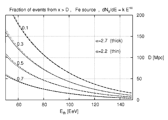
Figure 4: Considering the events arriving with energies above $E_{th}$, the contours indicate the fraction originating from distances larger than $D$, assuming a uniform distribution of Fe sources with similar intensities.

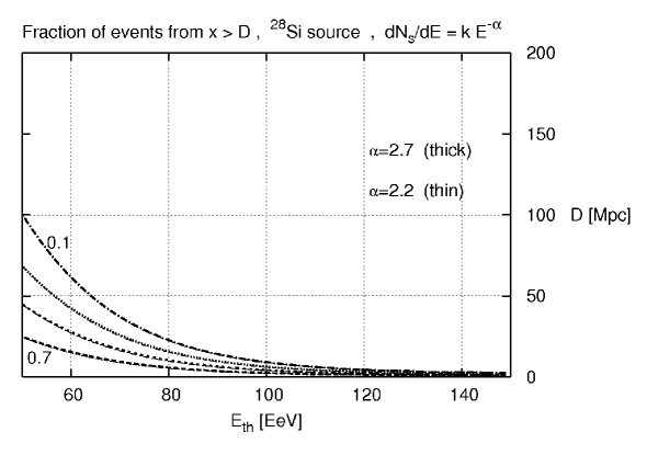
Figure 5: Considering the events arriving with energies above $E_{th}$, the contours indicate the fraction originating from distances larger than $D$, assuming a uniform distribution of Si sources with similar intensities.

In fig. 4 we depict the horizons for sources producing fluxes of Fe nuclei, obtained by following a large number of CRs with energies distributed according to the assumed spectra and obtaining the attenuation factors and associated fractions, as done before for the proton sources (fig. 2). For the evolution of the mass number we use eq. (8), while for the energies we account also for pair creation losses. In the Fe source case the horizons result smaller than for proton sources and they become even smaller for lighter nuclei, for which the attenuation lengths become shorter at the energies we are considering (fig. 3). This is illustrated in fig. 5, corresponding to the case of ²⁸Si sources. It is clear that in a realistic situation the actual fractions will depend on the details of the non-homogeneous local source distribution and on the source intensities, but the limiting distances from which CRs can arrive above a given threshold are quite insensitive to these details.

To better understand these results we show in figs. 6 the energies as a function of distance for a set of 50 CRs with initial energies sampling an $E^{-2.7}$ spectrum for the three cases discussed (p, Fe and Si). The results in figs. 2, 4 and 5 can then be interpreted naturally.

Figure 6: Energies as a function of distance to the source for a sample of initial energies. Top figure is for protons and bottom ones for Fe and Si sources (note the different horizontal ranges).

An important difference between the proton and nuclei results is related to the fact that when a nuclear species is above the threshold of the giant dipole resonance for a typical CMB photon, also the fragments from the photodisintegration will be above threshold (neglecting the subdominant energy losses due to pair creation) and hence the disintegration continues efficiently until the nucleus is completely disintegrated. On the contrary, nucleons which are originally above the threshold for photo-pion production and loose energy by pion emission may soon end up below threshold and hence continue their travel without further losses due to pion production. This leads to the well known pile-up in the proton spectrum, which is well seen in the top panel of fig. (6), a feature which is much less pronounced in the case of nuclei. This effect is also responsible for the smaller sensitivity of the results in figs. 4 and 5 to the adopted spectral index.

It is interesting to note that even if these scenarios adopt a single nuclear mass at the sources, the distribution of the masses of the CRs arriving to the Earth is quite wide, with contributions from many different nuclear species. This is exemplified in fig. 7, which displays the relative distribution of mass fragments arriving to the Earth above a threshold energy of 60 EeV for scenarios with Fe (dashed histogram) and Si (solid histogram) sources, with spectral index $\alpha=2.7$ (the results are not very sensitive to the value of $\alpha$ adopted).

The flux of secondary nucleons produced in the various photodisintegration processes is generally quite suppressed, since these nucleons will be emitted with energies $E/A$ if the CR started with energy $E$ and mass $A$. Hence, the secondary nucleons can contribute non-negligibly to the CR fluxes only in the case of very hard spectra ($\alpha\simeq 2$) and high source cutoffs ($E_{max}\gg AE_{th}$). For simplicity, we have just assumed in our computation that the maximum energy attained in the sources is $E_{max}=AE_{th}$ (which is bigger than $10^{21}$ eV in the examples considered), and in this case the secondary nucleons are always below threshold.

Figure 7: Distribution of masses of the fragments arriving to the Earth with $E>60$ EeV in a scenario with uniformly distributed Fe (dashed) and Si (solid) sources with spectral slope $\alpha=2.7$ (arbitrary units).

It is also worth mentioning that, as is seen from fig. 3, heavy nuclei produced with energies $E>A\times 10$ EeV have attenuation lengths of only a few Mpc. Hence, these nuclei will be essentially completely disintegrated after traveling $\sim 10$ Mpc. Since each nucleus of initial mass $A$ and energy $E$ will lead to $A$ nucleons with energies $E/A$, the number of nucleons above an energy threshold $E_{0}$ will be in this case $N(>E_{0})\simeq AN_{A}(>AE_{0})$, with $N_{A}(>E)\propto E^{1-\alpha}$ being the original integral source spectra (assuming here that the power law flux has no upper cutoff). We hence learn that the sources of nuclei farther than $10$ Mpc will produce a flux of secondary nucleons above 10 EeV similar to the source flux but suppressed by a factor $A^{2-\alpha}$, and extending up to energies $E_{max}/A$. The attenuation of these secondary nucleons caused by photo-pion and pair creation losses may then be studied as done in section 2.

Let us finally mention that both pair production losses and photo-disintegrations with the IR background have a significant impact, especially for the lower thresholds considered, on the results for Fe nuclei (fig. 4), while in the case of Si sources (fig. 5) their effect is less important.

4 Conclusions

As a summary, we have shown that the sources of the vast majority of the CR events observed with energies above 50 EeV should be at relatively close distances (under the plausible assumption that CRs consist of ordinary nucleons or nuclei), as is illustrated in a quantitative way in figs. 2, 4 and 5. These results should be relevant in order to restrict the distances to the candidate astrophysical objects that could act as sources for the observed ultra-high energy cosmic rays.

References

- [1] K. Greisen, Phys. Rev. Lett. 16 (1966) 748; G. T. Zatsepin and V. A. Kuzmin, JETP Lett. 4 (1966) 78.
- [2] F. Stecker, Phys. Rev. Lett. 21 (1968) 1016.
- [3] C. Hill and D. Schramm, Phys. Rev. D 31 (1985) 564.
- [4] V. Berezinsky and S. Grigorieva, Astron. Astrophys. 199 (1988) 1.
- [5] V. Berezinsky, S. Grigorieva and V. A. Dogiel, Astron. Astrophys. 232 (1990) 582.
- [6] F. Aharonian, B. Kanevsky and V. Vardanian, Astrophys. Space Sci. 167 (1990) 93.
- [7] S. Yoshida and M. Teshima, Prog. Theor. Phys. 89 (1993) 833.
- [8] J. P. Rachen and P. Biermann, Astron. Astrophys. 272 (1993) 161.
- [9] F. Aharonian and J. Cronin, Phys. Rev. D 50 (1994) 1892.
- [10] E. Waxman, Astrophys. J. 452 (1995) L1.
- [11] V. Berezinsky, A. Z. Gazizov and S. I. Grigorieva, Phys. Lett. B612 (2005) 147.
- [12] J. L. Puget, F. Stecker and J. H. Bredekamp, Astrophys. J. 295 (1976) 638.
- [13] L. N. Epele and E. Roulet, JHEP 9810 (1998) 009.
- [14] F. Stecker and M. H. Salamon, Astrophys. J. 512 (1999) 521.
- [15] E. Khan et al., Astropart. Phys. 23 (2005) 191.
- [16] D. Hooper, S. Sarkar and A. Taylor, astro-ph/0608085.
- [17] D. Allard et al., Astron. Astrophys. 443 (2005) L29.
- [18] D. Allard et al., JCAP 0609 (2006) 005.
- [19] G. Blumenthal, Phys. Rev. D 1 (1970) 1596.
- [20] M. J. Chodorowski, A. A. Zdziarski and M. Sikora, Astrophys. J. 400 (1992) 181.
- [21] M. A. Malkan and F. Stecker, Astrophys. J. 555 (2001) 641.
- [22] E. Waxman, K. Fisher and T. Piran, Astrophys. J. 483 (1997) 1.
- [23] A. Cuoco et al., JCAP01 (2006) 009.