The Magnificent Seven in the dusty prairie

Abstract

The Magnificent Seven have all been discovered by their exceptional soft X-ray spectra and high ratios of X-ray to optical flux. They all are considered to be nearby sources. Searching for similar objects with larger distances, one expects larger interstellar absorption resulting in harder X-ray counterparts. Current interstellar absorption treatment depends on chosen abundances and scattering cross-sections of the elements as well as on the 3D distribution of the interstellar medium. After a discussion of these factors we use the comprehensive 3D measurements of the Local Bubble by Lallement et al. (2003) to construct two simple models of the 3D distribution of the hydrogen column density. We test these models by using a set of soft X-ray sources with known distances. Finally, we discuss possible applications for distance estimations and population synthesis studies.

1 Introduction

The Magnificent Seven (M7), as the ROSAT-discovered X-ray thermal isolated neutron stars are sometimes dubbed, are exceptional because of their soft blackbody-like spectra without non-thermal components; for reviews see e.g. Haberl 2006 (this volume) or Haberl (2004). One of them has the second-best blackbody spectrum after the cosmic background radiation and this lead to one of the best neutron star radius estimates known (Trümper et al., 2004). Thought to be nearby, the M7 represent nearly half of the local young neutron star population. Despite several searches for new candidates of this radio-quiet neutron star class (e.g. Agüeros et al. 2006; Chieregato et al. 2005; Rutledge et al. 2003), no new M7-like object has been confirmed up to now. One aggravating circumstance these searches face is the hardening of the X-ray spectrum due to the interstellar absorption. Caused mainly by photo-electric absorption of photons by heavy elements, the interstellar absorption is usually described by the equivalent hydrogen column density assuming certain chemical abundances. Highly important is the clumpiness of the interstellar medium (ISM) causing (un)favourable lines of sights to search for new M7-like objects. The knowledge about the local ISM structure is also important in connection with the long-debated issue of isolated neutron stars accreting from the ISM.

1.1 Abundances and cross-sections

Most absorption models today presume element abundances independent of the line of sight. It was outlined by Wilms et al. (2000) that the total gas plus dust ISM abundances are lower than the local – Solar – abundances and the general ISM abundance uncertainties are still in the order of 0.1 dex because the measurements are very difficult. One can choose between several different abundance tables implemented e.g. in $XSPEC$ for analysing X-ray spectra. We note here only two examples commonly used – the abundance tables by Anders & Grevesse (1989) (’angr’ in $XSPEC$) and by Wilms et al. (2000) (’wilm’ in $XSPEC$) considering newer measurements by e.g. Snow & Witt (1996); Cardelli et al. (1996); Meyer et al. (1997, 1998).
The individual abundances and photoionization cross-sections of the elements and their ions as well as dust grain properties (e.g. sizes, shapes) influence the total photo-electric absorption of X-rays. Again, we mention here only two examplary works used very often for analysis of X-ray spectra. Morrison & McCammon (1983) did a polynomial fit of the effective absorption cross-section per hydrogen atom based on measured atomic absorption cross-sections by Henke et al. (1982) and abundances mostly from Anders & Ebihara (1982). With the exception of oxygen, Morrison & McCammon (1983) assume the elements to be either entirely in the gas phase or completely depleted into dust grains. The recent improved absorption treatment by Wilms et al. (2000) takes into account newer element abundances as noted above and more recent photoionization cross-section calculations by e.g. Verner et al. (1993); Verner & Yakovlev (1995). Wilms et al. (2000) additionally include an improved molecular cross-section for $H_{2}$. Besides this updated database Wilms et al. (2000) considered furthermore a simple spherical composite dust grain model in an MRN distribution (Mathis et al., 1977).
Both models are implemented in $XSPEC$ and can be used via the routines ’$wabs$’ (Morrison & McCammon, 1983) or ’$tbabs$’ (Wilms et al., 2000). The various absorption descriptions can lead to different results (see Fig. 1) or expectations of e.g. observable objects. The differences caused by the diverse treatments show our incomplete knowledge about the interstellar absorption and should be kept in mind especially when interpreting soft X-ray spectra.

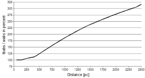
Figure 1: The effect of different abundances and cross-sections on the absorption towards soft X-ray sources
For the same neutron star (blackbody of 90 eV, 11.67 km radius, and 1.48 Solar masses) the ratio of the X-ray fluxes (as would be expected to be observed by ROSAT) resulting from the two $XSPEC$ routines ’$tbabs$’ and ’$wabs$’ are calculated for different distances. The galactic coordinate $x$ varies from 50 to 2500  pc (direction: from the Sun towards the galactic center), $y$ is always 0, $z$ is 25 pc north . For the ISM distribution, we applied the same as used by Popov et al. (2000), which is described in more detail below. The effect of less absorption, resulting from the use of the newer routine ’tbabs’, is stronger at larger column densities, hence distances.

1.2 The inhomogeneously distributed ISM

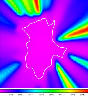
Figure 2: The limits of using the Ferlet et al. (1985) formula
The sodium column density as derived from the density data by Lallement et al. (2003) is shown in galactic cartesian coordinates at z=0; x is towards the galactic center which is at the right, y towards l=90^∘ is pointing up. The image spans 500 pc times 500 pc. The area within the contour has low column densities ($\log$ N$(NaI)<11$) for which Welty et al. (1994) doubted whether the Ferlet et al. (1985) formula is applicable. This region of small sodium column densities is largest at z=0 and becomes smaller for lower or larger z.

In X-ray astronomy with low spectroscopic resolution the chosen abundances and cross-sections are used to derive the hydrogen column density responsible for the instellar absorption. Cold and warm H-atoms (H i ) as well as hydrogen molecules and ionized hydrogen (H ii ) contribute to the overall amount of hydrogen along a line of sight. These different components of the hydrogen column density are estimated by different measurement methods, e.g. various extinction measurements as summarized by Knude (2002) or radio 21-cm observations of hydrogen as the extensive study by Dickey & Lockman (1990) and more recently by Kalberla et al. (2005). A wealth of theoretical models has been applied to these observations. However, most of them are only 2D with few more recent exceptions (see e.g. Drimmel et al. 2003, Amôres & Lépine 2005 or Marshall et al. 2006 for 3D models). The overall result is a highly inhomogeneously distributed interstellar medium within the Milky Way, present in bubbles with loops or dense rims, and shaped by molecular clouds, supernova explosions and stellar activity (for an illustrated overview see Henbest & Couper 1994). The ISM distribution is best known in the close Solar neighbourhood, especially in the Local Bubble (e.g. Breitschwerdt 1998). The most detailed view is provided by the study of Lallement et al. (2003), who measured Na i absorption towards 1005 sightlines with Hipparcos distances up to 350 pc from the Sun; for more details on the measurements and the applied density inversion method see Lallement et al. (2003), the precursor paper Sfeir et al. (1999), and Vergely et al. (2001). Nai is regarded as good tracer of the total amount of the neutral interstellar gas and the sodium column density is thought to be convertable into a hydrogen column density (e.g. Ferlet et al. (1985), but see also discussion in sec. 2). For more distant regions the determination of a 3D distribution of the ISM is hampered mainly by the unknown or imprecise distances of the measured objects and the lack of a well-sampled grid of measurement points. This is true for all extinction-related methods to our knowledge and results in much more coarse sampling compared to the Solar neighbourhood. The results obtained by the various methods can differ for the same regions and a combination can be difficult. These difficulties result partly from the different observed astrophysical phenomena like measuring the dust emission or stellar magnitudes. They also result from different sets of stellar absolute magnitude calibrations and the underlying assumptions which can deviate from each other as interstellar extinction determination is an iterative process coupled with the identification of the statistical properties of stars (Hakkila et al., 1997).

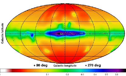
Figure 3: The N(H) predicted by the analytical model at 1 kpc
Positive galactic latitudes are up and $l=0^{\circ}$ is in the center. The N(H)is in units of $10^{22}$cm^-2. For description of the model and discussion see text.

2 Two simple 3D distribution model cubes of the absorbing ISM

Considering the absorption in the Solar neighbourhood, the result by Lallement et al. (2003) is a good starting point representing the currently best database of the local ISM distribution. R. Lallement kindly provided us with the Nai density cube derived using the inversion method developed by Vergely et al. (2001). Due to the smoothing length of 25 pc applied in this method by Lallement et al. (2003), structures smaller than 25 pc cannot be resolved. We note further that even if measurements go up to Hipparcos distances of 350 pc from the Sun, the sampling becomes coarser at larger distances. Thus the sodium density cube has a span of only 250 pc and starting from 200 pc one has to be careful dealing eventually with the a priori density information applied in the inversion method (R. Lallement, personal communication). From the Nai density cube we calculate the column density for the same grid (sampling 3.9 pc). This is then converted to H i column density applying the formula by Ferlet et al. (1985).

It has to be mentioned that there are on-going discussions about how well the sodium D-line absorption actually traces H i . The correlation found between the H i and Na column densities derived from Na-D absorption lines by Ferlet et al. (1985) was doubted by Welty et al. (1994), especially for low column densities ($\log$ N$(NaI)<11$). The region of the Lallement cube that should not be used because it has such low column densities is indicated in Fig. 2.

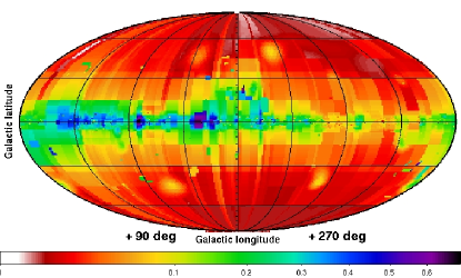
Figure 4: The N(H) predicted by the extinction model based on Hakkila et al. (1997) at 1 kpc
Positive galactic latitudes are up and $l=0^{\circ}$ is in the center. The N(H) scale is in unities of $10^{22}$cm^-2. For description of the model and discussion see text.

However, the lowest known X-ray–measured hydrogen column density for one of the M7 converts to a sodium column density of $\log$ N(Nai) $>11.5$ (applying the formula by Ferlet et al. 1985). Therefore this low-column density uncertainty is not important considering the M7 and negligible for the intended population synthesis with neutron stars (NSs) at usually larger distances.
Vergely et al. (2001) could not always find a correlation of the Nai density with the H i density. They concluded that the correlation is rather weak due to non-constant population ratios for interstellar medium species, thus different abundances. Lallement et al. (2003) noted the size of the Local Bubble revealed by H i is smaller than when derived by Nai. This was explained by the first ionization stage of Nai being below that of H i , resulting in a longer neutral phase of H i (Lallement et al., 2003). Recently, Hunter et al. (2006) presented new ultraviolet Nai observations towards 74 O- and B-type stars in the galactic disk. Where possible they also derived column densities of the Nai D-lines. Then they compared the correlation between the Nai and H i column densities. While there was an excellent agreement with Ferlet et al. (1985) for the D-lines, this was not the case for their ultraviolet absorption lines. Hunter et al. (2006) found a significant offset for the correlation they got from the Nai D-lines compared to the relation derived from the UV transitions, even after accounting for saturation effects in the D-lines. They argue that this offset is due to an underestimation of approximately 30 $\%$ of N(H) in the case of Nai D-lines observations. Recapitulating, one has to be aware of the still not completely solved problems concerning the conversion of Nai to H i column densities when it comes to interpreting individual results. However, we regard the measurements by Lallement et al. (2003) and the conversion to a hydrogen column density according to Ferlet et al. (1985) as the best possibility at hand to take into account the local inhomogenity in the ISM for X-ray astronomy with low spectral resolution.

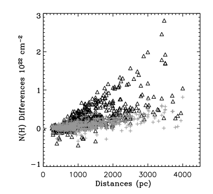
Figure 5: N(H) deviations at different distances
Shown are the differences between the model N(H) at the distances of the open cluster sample and the N(H) obtained directly from the reddening measurements of this sample. The results of the extinction model based on Hakkila et al. (1997) are plotted as grey crosses, those of the analytical model as black triangles. While the scatter at low distances is relatively small, the analytical model has a larger spread at larger distances.

At larger distances we consider two different models – one is based completely on extinction measurements and another one is described by analytical formulae. Hakkila et al. (1997) put several extinction studies carefully together in an easily accessible routine. All studies have been modified to statistically account for unsampled regions. Additionally, a correction method for the systematic underestimation between 1 and 5 kpc was developed. Errors were provided individually for each considered main survey and for their mean. The often large mean error values illustrate the disagreement among individual observations. The model by Hakkila et al. (1997) is a large scale model, capable of identifying e.g. molecular clouds at intermediate distances, but not sensitve to extinction variations of less than 1 degree. It is well suited for statistical studies.
The analytical model we apply is described by Popov et al. (2000). It is based on the formulae by (Zane et al., 1995; Dickey & Lockman, 1990; de Boer, 1991). Popov et al. (2000) included additionally a galactocentric radius dependency for the number density of atomic and molecular hydrogen as estimated by Bochkarev (1992). The Local Bubble was taken into account by Popov et al. (2000) as a sphere of 140 pc radius having a constant low density of 0.1 particles cm^-3. As noted above, there are other more recent theoretical 3D extinction models. However, the analytical $H$ density model by Popov et al. (2000) seems to be at least as good as e.g. the underlying model used by Amôres & Lépine (2005). The model of Drimmel et al. (2003) cannot be applied to distances less than a few hundred parsecs in the Solar neighbourhood and the data of Marshall et al. (2006) has a coarse sampling with distance bins of 1 kpc.
Both described models are applied only for distances larger than 230 pc in case they provide an N(H) larger than derived from the sodium cube at 230 pc. Otherwise the hydrogen column density at 230 pc is taken since the column density can only increase with distance. We use spherical coordinates – the galactic cordinates $l$, $b$ and distance $d$. The nominal sampling is one degree in $l$ and $b$, and 10 pc for the distance. This is technically motivated and does not represent the actually achieved accuracy. Distances are covered up to 4500 pc.

2.1 Testing the models and further improvements

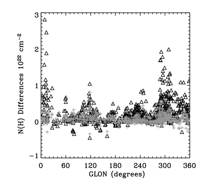
Figure 6: N(H) deviations at different galactic longitudes The symbols for the models are the same as in Fig. 5. For both models a larger scatter is visible at GLON$=0^{\circ}$,$120^{\circ}$, and $300^{\circ}$

To test our models we first consider a relatively large number of test objects with good distances and extinction measurements, not necessarily determined from X-rays. Then we proceed to a few of the rare neutron stars with well known distances, having also small error bars for the absorbing N(H) derived by X-ray observations.
As Hakkila et al. (1997) note, different studies do not agree precisely with each other due to the various applied methods or objects studied. The latter are usually very coarsely scattered and measurement errors can influence the extinction values of a large region. One possibility to overcome this problem is investigating open clusters. An open cluster has the advantage that one can measure a number of stars at approximately the same distance, which is usually well known. Therefore, open clusters are a good choice in aiming to minimize the extinction measurement errors along one line of sight. Usually one measures the reddening $E(B-V)$. We concentrate here on the recent comprehensive reddening measurements for 650 open clusters by Piskunov et al. (2006), representing a complete sample up to distances of about 850 pc from the Sun. Details about this open cluster study can be found in Piskunov et al. (2006); Kharchenko et al. (2005a, b). To convert the reddening $E(B-V)$ we apply the formula by Paresce (1984): $N(H)=5.5\times 10^{21}E(B-V)\left[\rm{cm}^{-2}\right]$. This is quite similar to the slope found in the X-ray study for the extinction $A_{V}$ by Predehl & Schmitt (1995): $N(H)=1.79\pm 0.03\times 10^{21}A_{V}-0.41\left[\rm{cm}^{-2}\right]$ if $A_{V}=3.1E(B-V)$. This is noted here because there is a deviation of the correlation by Predehl & Schmitt (1995) between $A_{V}$, indicator of the dust, and $N(H)$, indicator for cold gas and dust, at low distances. This is probably due to a significantly lower amount of dust in the Local Bubble, as also found by Predehl & Schmitt (1995) for the source LMC X-1. Therefore, we consider only open clusters with distances larger than 230 pc.

Table 1: Testing the models for individual objects
For each object the known distance and hydrogen column density N(H) with references are given. Furthermore are listed for each model: the obtained minimal distance D_MIN for the lowest N(H) value, the maximal distance D_MAX for the largest N(H) value and the expected N(H) for the known distance. The models are the same up to a distance of 230 pc (see text for details). The first 4 objects are neutron stars with VLBI or HST parallaxes and X-ray–obtained N(H). TY CrA lies within the CrA star forming molecular cloud core close to RX J1856.5-37541. HD 18190 is thought to be situated behind MBM 12.
1: Golden et al. (2005); 2: Marshall & Schulz (2002); 3: Dodson et al. (2003); 4: Pavlov et al. (2001); 5: Caraveo et al. (1996); 6: Jackson & Halpern (2005); 7: Kaplan et al. (2002); 8: our EPIC-pn fit; 9: Casey et al. (1998); 10: Forbrich et al. (2006); 11: Hobbs et al. (1988);
^a $log($N(Nai$))=10.6<11$ Ferlet et al. (1985) formula was doubted by Welty et al. (1994), see text; ^b note the recently refined parallax by van Kerkwijk & Kaplan (2006) yielding a distance of $161^{+18}_{-14}$ pc; ^c mean value; ^d lower limit for N(Nai) was converted to N(H); $out$: needed N(H) is not reached up to the here considered 1 kpc distance

Name	Distance	Ref.	N(H)	Ref.	analytical model			extinction model
					DMIN	DMAX	N(H)	DMIN	DMAX	N(H)
	[pc]		[$10^{20}$ cm-2]		[pc]	[pc]	[$10^{20}$ cm-2]	[pc]	[pc]	[$10^{20}$ cm-2]
PSR B0656+14	$288^{+33}_{-27}$	1	$1.73\pm 0.18$	2	240	260	2.68	230	240	2.86
Vela	$287^{+59}_{-34}$	3	$3.3\pm 0.3$	4	300	330	2.73	860	910	1.07
Geminga	$157^{+19}_{-17}$	5	$1.76\pm 0.95$	6	220	300	0.09a	220	240	0.09a
RX J1856.5-37541	${140\pm 40}$b	7	$0.74\pm 0.10$	8	130	140	0.87	130	140	0.87
TY CrA	$129\pm 11$	9	$130\pm 0.3$c	10	out	out	0.08	out	out	0.08
HD 18190	185	11	$>7.21^{d}$	11	440	$\cdots$	5.05	800	$\cdots$	5.05

We compared the hydrogen column densities we inferred from the open cluster reddenings with those obtained by the models. 628 out of the 650 open clusters by Piskunov et al. (2006) lie within the considered data cube with distances larger than 230 pc and smaller than 4.5 kpc. The scatter in the obtained extinction differences increases with distances for both models (see Fig. 5). For the model based on Hakkila et al. (1997) the mean deviation is around $9\cdot 10^{20}$ cm^-2, the corresponding mean value for the analytical model is $27\cdot 10^{20}$ cm^-2. Considering only distances up to 1 kpc these values are $3.3\cdot 10^{20}$ cm^-2 and $8.1\cdot 10^{20}$ cm^-2 respectively. Interestingly at some galactic longitudes ($l\approx 0^{\circ}$, $120^{\circ}$, and $300^{\circ}$; see Fig. 6) and at the galactic latitude $b\approx 0^{\circ}$ the scatter is more pronounced. The extinction routine by Hakkila et al. (1997) predicts the observed properties of the open clusters better than the analytical model. This can be partly explained by the use of (older) open cluster data (e.g. Fitzgerald 1968) in the routine by Hakkila et al. (1997). The analytical model tends to overpredict the extinction by an order of magnitude, especially at larger distances. Due to the convincing advantages of extinction data derived from open clusters, we include them finally as local inhomogenities in our models for distances larger than 230 pc. Again, we take into account that the column density can only increase with distance. If N(H) outside 230 pc is lower than the value at 230 pc in this direction we consequently changed the values based on the Lallement et al. (2003) to the lower value until an N(H) increasing homogeneously with distance is reached. Aiming to apply our N(H)-models to X-ray detected neutron stars their performance for well known sources is interesting. We selected four of the rare NSs having at the same time known parallaxes and hydrogen column densities with small error bars obtained from X-ray observations. In Table 2.1 we present the model-derived distances for the measured N(H) range as well as the model-derived N(H) at the given parallactic distance. While the analytical model gives reasonable results for PSR B0656+14, Vela and RX J1856.5-37541 (RXJ1856 in the following), the extinction model based on Hakkila et al. (1997) underestimates the column density towards Vela significantly. As both ISM models are equal up to 230 pc, both give the same minimal distance of 220 pc towards Geminga which deviates from the claimed distance by Caraveo et al. (1996). Interestingly Walter et al. 2006 (this volume) reported recently a revised distance of $254^{+111}_{-59}$ pc towards Geminga. In the case of RXJ1856 the derived minimal and maximal distances are completely included in the N(H) cube obtained by the Lallement et al. (2003) measurements. Here, an error of 25 pc applies while an error estimate is difficult for the analytical model at distances larger than 230 pc. The Hakkila et al. (1997) model has often a formal mean error of the same order as the obtained N(H) values.

As noted in above it is still debated how good Nai D-lines are as tracer for hydrogen. In particular it is unclear whether molecular hydrogen is well traced. In Table 2.1 we include the results obtained for two further test objects situated in or close to molecular cloud cores – the star-forming site CrA close to RXJ1856 and MBM12 (Magnani et al., 1985). While towards MBM12 there is an enlarged but still underestimated amount of hydrogen (see also Lallement et al. 2003 for discussion of MBM12), the small CrA cloud is clearly missed. Both examples indicate that one has to be cautious in applying the $N(H)$ cube obtained from the Lallement et al. (2003) measurements in the direction of small molecular clouds. However, there are only few such density enhancements of molecular hydrogen in the close Solar neighbourhood. The extinction model as well as the analytical model are in principle sensitive to molecular hydrogen. At large distances $>1$ kpc the extinction model may miss molecular clouds due to their low angular size and bad sampling while the analytical model does not consider individual clouds.

3 Applications of the models

3.1 Distance estimates

A possible application is to estimate the distance to neutron stars without parallaxes or other distance measurements. This is the case of the majority of the M7 where despite for RXJ1856 only a preliminary parallactic distance of $330^{+170}_{-80}$ pc is reported for RX J0720.4-3125 by van Kerkwijk & Kaplan 2006 (this volume). We obtain N(H) by considering the best $XSPEC$-fits for blackbody and absorption lines of all currently available XMM EPIC-pn observations reduced with XMM SAS 6.5 for each neutron star. As noted by Haberl 2006 (this volume), in this respect the XMM EPIC-pn is the best-suited instrument for relative measurements with reasonably small errors ($\approx 0.1\cdot 10^{20}$ cm^-2 for all objects). The model predictions for these column densities can be found in Table 3.1. As noted before, the technical sampling is 10 pc. If a N(H) value lies between two sampling points we indicate this by noting e.g. 235. However, even errors in the best-studied regions ($\leq 230$ pc) are around 25 pc , and can be much larger otherwise.

Table 2: Distances obtained for the M7 The N(H) was obtained by blackbody and absorption line ($tabs$) $XSPEC$-fits from XMM-$Newton$ EPIC-pn observations (abundances and cross-sections are chosen according to Wilms et al. 2000). The number of lines used is indicated in parenthesis. The corresponding model prediction of the distance is given for the analytical model: d_ana, the extinction model based on Hakkila et al. (1997) d_ext, and the analytical model plus consideration of possible 30% underprediction by the sodium D-lines: d_ana130. See also text for discussion.

name	N(H) ($\#$lines)	dana	dext	dana130
	[$10^{20}$ cm${}^{-2}]$	[pc]	[pc]	[pc]
RX J1856.5-3754	0.7 (0L)	135	135	125
RX J0420.0-5022	1.6 (1L)	345	$\cdots$	325
RX J0720.4-3125	1.2 (1L)	270	235	265
RX J0806.4-4123	1.0 (1L)	250	235	240
RBS 1223	4.3 (1L)	$\cdots$	$\cdots$	$\cdots$
RX J1605.3+3249	2.0 (3L)	390	$\cdots$	325
RBS 1774	2.4 (1L)	430	$\cdots$	390

In case of the extinction model based on Hakkila et al. (1997) one cannot always derive a convincing value due to bad sampling with the (low) extinction not changing over a large scale of distances (e.g. up to 1 kpc). For the analytical model only the high latitude object RBS 1223 is a problem where at 1 kpc one arrives only at $3.2\cdot 10^{20}$ cm^-2. The limitations of this large-scale model appear here. However, absorption lines in the spectrum also influence N(H). Schwope 2006 (this volume) fitted the spectrum of RBS 1223 using recent new observations and obtained N(H)$=3.7\cdot 10^{20}$ cm^-2 for one absorption line. This value is comparable to our result in Table 3.1, taking into account the additional data. However, the fit was not very good and Schwope 2006 obtained better fits with two absorption lines N(H), yielding values ranging from $1.2\cdot 10^{20}$ cm^-2 to $1.8\cdot 10^{20}$ cm^-2. The lower value would correspond to a distance of 525 pc when using the analytical model

Overall, the distances derived from both models towards two neutron stars are in acceptable agreement: for RX J0720.4-3125 with 250 pc and for RX J0806.4-4123 with 240 pc. Since both NSs are close to the border of the sodium measurements, an error of $\approx 25$ pc seems reasonable. In general, the values of the analytical model have to be used with caution as local clumpiness of the ISM is not considered by this model at distances $>230$ pc. Considering the open cluster test from above, the mean N(H) deviation of the analytical model up to 500 pc is $0.05\cdot 10^{20}$ cm^-2; the standard deviation, however, is $4.9\cdot 10^{20}$ cm^-2.

3.2 Population synthesis

Figure 7: The log$N$–log$S$ curves for different models Each curve shows the expected number of observable neutron stars at ROSAT PSPC countrates. The solid line represents the curve for the new progenitor distribution but old absorption model; the dotted and the dashed line are the results of the old simulations by e.g. Popov et al. (2003) for Gould Belt radii of $R_{GB}=500$ pc and $R_{GB}=300$ pc respectively. The only difference to the solid curve is the progenitor distribution. The results of taking into account the new progenitor distribution and additionnally the new absorption models are shown by the dashed-dotted line for the refined analytical ISM model and the dot-dot-dot-dashed line for the extinction model based on Hakkila et al. (1997). Furthermore the measurement points of young NSs with thermal X-ray emission are plotted as in Popov et al. (2003). For discussion see text.

The main motivation for us to take into account better absorption treatment is an improved population synthesis model based on that of Popov et al. (2000, 2003) and Popov et al. (2005c). A detailed discussion of the improvements is beyond the scope of this article and will be provided elsewhere (Popov, Posselt, in preparation). Therefore, we summarize here only the new developments and concentrate on illustrating the importance of the interstellar absorption. While Popov et al. (2003, 2005c) modeled the neutron star progenitor distribution as coming from infinitely thin disks, either from the galactic plane or the Gould Belt, the new initial distribution is more realistic. Up to the Hipparcos limit of 400 pc (ESA, 1997) the known B2-O8 stars are considered individually as well as their affiliation to an OB association (de Zeeuw et al., 1999) resulting in birth properties depending on the age of the OB-association. The Gould Belt birth rate is applied here. For distances above 400 pc, the galactic disk is considered for few neutron stars randomly as well as 36 associations (Blaha & Humphreys, 1989; Mel’nik & Efremov, 1995) for most of the neutron stars. Due to the unknown ages of the associations, the birth probability is set proportional to the number of association members. In Fig. 7, the log$N$-log$S$ curves are shown for the old thin-disk Gould Belt models with either 300 pc or 500 pc radius, the new progenitor distribution as well as for the the new progenitor distribution considering both absorption models. All simulations were done for the same mass spectrum as in Popov et al. (2006), the cooling curve set labeled Model I in the same paper, the same abundances and cross-sections (in this case those of Morrison & McCammon (1983) for comparison) and identical remaining parameters. The results for the new progenitor distribution lie in-between those of the two Gould Belt sizes, a little apart from the measured integrated number of objects. This is also true for the curve considering the absorption by the analytical model. At the bright end the differences introduced by the analytical absorption model are only very small. Towards lower countrates, the curve lies significantly below the one without the refined 3D ISM model. Considering the absorption based on the extinction model by Hakkila et al. (1997) gives another picture. At the bright end the curve is much lower than that without the refined 3D ISM model, while the difference becomes smaller towards low countrates. We note here again that both absorption models are the same up to 230 pc, based on the measurements by Lallement et al. (2003). Both also consider the open cluster data, however slightly differently as the column density is only allowed to increase. The curve of the analytical model shows best the influence of an improved ISM distribution model compared to the old absorption treatment (e.g. Popov et al. 2003) where the analytical model without the data by Lallement et al. (2003) and Piskunov et al. (2006) was used). One might have expected that differences should be largest at low distances and hence for bright sources. However, averaging over the small Local Bubble gives apparently the same result as the simpler description before. The influence of the better model for the Solar vicinity is apparent in the expected location likelihoods for neutron stars. Going to larger distances the additive column densities are especially large around $l\approx 300^{\circ}$ to $l\approx 60^{\circ}$ in the galactic plane where many objects could be expected. Thus, the number of predicted neutron stars is reduced. The N(H) model based on the extinction study by Hakkila et al. (1997) shows on average much higher N(H) already at 240 pc compared to the analytical model. Given the nearly rectangular shape of the regions with relatively high values in the $l,b$ plane these seem to be caused at least partly by bad sampling and the necessary statistical treatment. The higher N(H) results in less observable sources bringing the corresponding log$N$-log$S$ much closer to the actually measured number of sources at the bright end. We made similar test plots for the expected neutron star number per square degree like the one presented in Fig. 6 by Popov et al. (2005c). We summarize here only the main results, for detailed discussion see Popov, Posselt 2006 (in prep.). Contrary to the old model the predicted neutron star number is enhanced in regions including the nearby Gould Belt OB associations (e.g. Upp Sco) with the new progenitor distribution. Sources are not anymore homogeneously distributed at all longitudes along the planes of the galactic disk or the Gould Belt. When it comes to consider the 3D ISM models, the influence of the absorption is on much smaller scales. Less sources would be expected at higher latitudes, and towards some small regions the high extinction hinders the possible detection of neutron stars. Differences between the two absorption models are pronounced only in small regions which to discuss in detail is beyond our intention here.

4 Conclusions

An understanding of the interstellar absorption is crucial for the interpretation of low-resolution soft X-ray spectra. Taking into account the 3D distribution of the ISM is important to determine the absorption of known sources as well as for searches of new soft X-ray sources towards a particular direction in the sky. We presented two simple models for 3D ISM distributions together with possible applications: distance estimation and the population synthesis for young isolated thermal, thus soft X-rays emitting neutron stars. Both models are large scale models and have to be used with caution especially considering distance estimations. Concerning population synthesis the two models influence the log$N$–log$S$ curve discriminatively, while the differences for the predicted spatial distribution of observable neutron stars are only small.