On the Age of Stars Harboring Transiting Planets

Results of photometric surveys have brought to light the existence of a population of giant planets orbiting their host stars even closer than the hot Jupiters (HJ), with orbital periods below 3 days. The reason why radial velocity surveys were not able to detect these very-hot Jupiters (VHJ) is under discussion. A possible explanation is that these close-in planets are short-lived, being evaporated on short time-scales due to UV flux of their host stars. In this case, stars hosting transiting VHJ planets would be systematically younger than those in the radial velocity sample. We have used the UVES spectrograph (VLT-UT2 telescope) to obtain high resolution spectra of 5 faint stars hosting transiting planets, namely, OGLE-TR-10, 56, 111, 113 and TrES-1. Previously obtained CORALIE spectra of HD189733, and published data on the other transiting planet-hosts were also used. The immediate objective is to estimate ages via Li abundances, using the Ca II activity-age relation, and from the analysis of the stellar rotational velocity. For the stars for which we have spectra, Li abundances were computed as in Israelian et al. (2004) using the stellar parameters derived in Santos et al. (2006). The chromospheric activity index $S_{US}$ was built as the ratio of the flux within the core of the Ca II H & K lines and the flux in two nearby continuum regions. The index $S_{US}$ was calibrated to Mount Wilson index $S_{MW}$ allowing the computation of the Ca II H & K corrected for the photospheric contribution. These values were then used to derive the ages by means of the Henry et al. (1996) activity-age relation. Bearing in mind the limitations of the ages derived by Li abundances, chromospheric activity, and stellar rotational velocities, none of the stars studied in this paper seem to be younger than 0.5 Gyr.

1 Introduction

Since the discovery of 51Peg b by Mayor & Queloz (1995) the number of new extra- solar planets has been rapidly growing. More than about 160 extra-solar planets have been found and yet none of them look like our paradigm for planetary formation, i.e., the Solar System. On the contrary, these new discoveries provide evidence that a large variety of orbital characteristics probably related to their formation process are actually possible.

Due to the considerable number of giant planets found orbiting their host stars at short periods (typically below 10 days) it was soon realized that migration has to play a key role in their formation, since a solid core massive enough to accrete gas is not able to grow at such a short distance from the parent star (Pollack et al. 1996).With the increasing number of discoveries, statistical trends are arising, revealing interesting imprints thought to be left by the migration mechanism which brought these planets close-in (Udry et al. 2003). An annoying point when dealing with migration is how to stop it. The pile-up of planets with $P_{orb}\sim 3-3.5$ days in the the orbital period distribution was understood as an observational clue indicating the migration parking point. Although appealing, this interpretation was severely challenged by the discovery of the transiting planets. Some of these new transiting planets have more than a Jupiter mass but nevertheless they revolve around their host stars in an even shorter orbital period than the so-called Hot Jupiters (HJ), typically $P_{orb}\la 1-2$ days. For this reason, they have been called Very Hot Jupiters (VHJ).

Why these planets have not been detected more often by the radial velocity surveys is a matter of debate. Gaudi et al. (2005) advocate that the non-detection of VHJ by the radial velocity surveys is a statistical effect due to the much lower frequency of VHJ as compared to that of HJ.

Given their proximity to their host stars, the VHJ may experience some degree of evaporation due to the heating by stellar UV photons. Vidal-Madjar et al. (2004) showed that HD209458b is indeed evaporating, but due to saturation of the spectral lines, only an upper limit on the mass loss of 10${}^{10}\rm\,g\,s^{-1}$ can be derived. According to theoretical calculations, the extreme case of an efficient heating of the planet atmosphere may lead to an energy-limited evaporation $\leavevmode\nobreak\ 10^{12}\rm\,g\,s^{-1}$ for HD209458b (Lammer et al. 2003), and hence to a very efficient evaporation, possibly to the total dissociation of some planets (Lecavelier des Etangs et al. 2004; Baraffe et al. 2004). Conversely, cooling in the atmosphere may well lead to a much more limited mass loss close to the lower limit derived by Vidal-Madjar et al. (Yelle 2004; Hubbard et al. 2005).

Is a catastrophic fate a possible explanation for the lack of planets with periods shorter that 3 days? The existence of the VHJ is an important constraint to this type of scenario. Evaporation scenarios must be able to explain the observed evaporation rate of HD 209458b, while at the same time accounting for the long-term survival of the VHJ on even closer orbits. One possibility is that VHJ are not viable in the long term and are fated to catastrophic evaporation. In this case the three observed VHJ would simply be too young to have evaporated yet.

The aim of the present article is to examine the likelihood of the hypothesis that the three VHJ were found around parent stars that are very young compared to typical planet host stars and to the time scales of evaporation. For this purpose, three indicators of young stellar ages are combined: i) chromospheric activity (e.g. Henry et al. 1996) ii) Lithium abundances and iii) rotational velocity.

The manuscript is organized as follows. Our observations and data reduction are described in Sec. 2. In Sec. 3 our index $S_{US}$ is built and calibrated with respect to the index $S$ of Mount Wilson $(S_{MW})$. In Sec. 4, we derive the Li abundances for the observed stars. Projected rotational velocities available in the literature for stars hosting transiting planets are compiled in Sec. 5. Using the different observables we derive ages in Sec. 6 and discuss the implications of the derived ages for the planetary evolution under evaporation in Sec. 7.

2 Observations

For 5 of the transiting planet host stars (OGLE-TR-10, 56, 111, 113 and TrES-1) the observations were carried out with the UVES spectrograph at the VLT-UT2 Kueyen telescope (program ID 75.C-0185), between April and May 2005 (in service mode). The Dichroic #1 390+580 mode was used. The red arm spectra cover the wavelength domain between 4780 and 6805Å, with a gap between 5730 and 5835Å, whereas the data obtained with blue arm cover the wavelength domain between 3260 and 4450Å. For all stars, we adopted slit widths of 0.9 arcsec and 1.1 arcsec, which provides a spectral resolution ($\lambda$/$\Delta\lambda$) of the order of 50 000 and 40 000 in the red and blue arm, respectively.

For each exposure, both the blue arm CCD and the red mosaic were read in 2x2 bins to reduce the readout noise and increase the number of counts in each bin. This procedure does not compromise the resolving power, since the sampling of the CCD is still higher (by a factor of 2) than the instrumental PSF. For the brighter TrES-1, we choose a 1x1 binning for the red arm CCD.

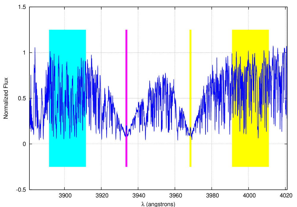
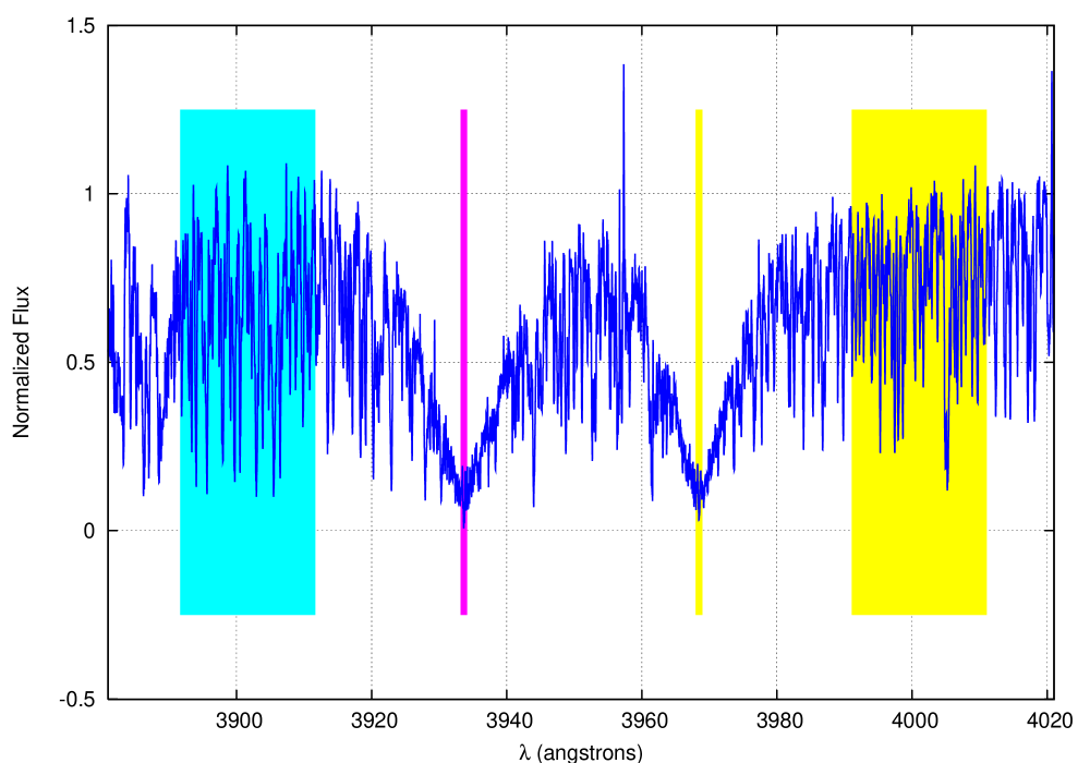
Figure 1: On line and continuum filters used in the computation of $S_{US}$. The UVES spectrum for TrES-1 (top panel) and OGLE-TR-10 are shown in the figure.

For the OGLE stars, particular attention was given to the orientation of the slit given the relative crowdedness of the fields. The angle was chosen in each case using the images available at the OGLE website, in order that no other star was present in the UVES slit.

Data reduction was carried out by the ESO staff using the UVES pipeline as part of the service mode data package.

Finally, for the analysis of HD189733 we have used the same CORALIE spectrum taken by Bouchy et al. (2005b).

3 Chromospheric Activity

Chromospheric ages are commonly derived using the age-chromospheric activity relation constructed based on the Mont Wilson (MW) chromospheric flux index ($S_{MW}$)(e.g. Vaughan et al. 1978; Henry et al. 1996). In order to use MW calibration, one needs first to build a chromospheric flux indicator (here called $S_{US}$) and then calibrate it with respect to the MW system ($S_{MW}$). This procedure has been carried out many times in different papers (e.g. Santos et al. 2000; Wright et al. 2004; Saffe et al. 2005). Here we follow the prescription of Santos et al. (2000).

The $S_{US}$ index is defined as $(F_{H}+F_{K})/(C_{H}+C_{K})$ where $F_{H}$ and $F_{K}$ are the sum of the fluxes within a 1-Å box centered on the Ca H and K lines, respectively. $C_{H}$ and $C_{K}$ are the total flux computed as for $F_{H}$ and $F_{K}$ but for 20-Å boxes centered at 4001.067Å and 3901.67Å , respectively. In order to calibrate $S_{US}$ as a function of $S_{MW}$ a number of common stars in both samples is needed. Our original sample observed with UVES contains only spectra of stars hosting transiting planets, therefore external data for calibrators is needed. HARPS spectra, kindly provided by the HARPS team, were used as calibrators. Therefore, as a prior step before computing the flux index, the HARPS spectra were smoothed to match the UVES blue-arm resolution of 40000 by convolving a gaussian profile with the appropriate width and the UVES data were rebinned to match the HARPS spectral sampling of 0.01Å .

Spectra of calibrators and planet host stars were brought to the rest frame using the radial velocities given by the cross-correlation function fit. The data were then trimmed from 3870Å up to 4070Å and normalized by a straight line within this interval. Finally the $S_{US}$ is computed by adding the relative intensity of the pixels within each filter. Figure 1 shows the spectral region used to compute $S_{US}$.

One might inquire whether a calibration built with data collected with one instrument can be used to calibrate a different one. The index $S$ simply measures the ratio between the flux in the core of the Ca II H and K lines with respect to a continuum region next to these lines. Therefore provided that i) the instrumental responses are correctly subtracted within the region containing the Ca II lines and the continuum, ii) the fluxes are computed exactly in the same way for both instruments and, iii) data have the same sampling and resolution, the indices S will reflect solely the stellar contribution regardless of the instrument used to collect the data.

Most of the instrumental contribution (blaze function, pixel-to-pixel variations, CCD response, etc.) is removed by the division of the extracted spectrum by the flat field spectrum. The remaining effects are subtracted by normalizing the reduced spectrum by a pseudo-continuum. Since the position of the true continuum is not known, the normalization process will certainly introduce errors in our computed $S$ and therefore in the final ages. In order to quantify how changes in the continuum are reflected in the computed $S_{US}$, we compared the $S_{US}$ values determined using the normalized and non-normalized spectra. In the worst cases the variations in the $S_{US}$ were of 5%. This error is much smaller than the variations of $S_{MW}$ which are typically of 20%.

As an additional check of the validity of our $S_{US}-S_{MW}$ calibration, we have compared the $S_{MW}$ derived using spectra collected with HARPS with those computed using spectra from the UVES POP spectral library (Bagnulo et al. 2003) for 6 stars in common. For 5 stars whose $S_{MW}$ is below 0.2, the differences in the $S_{MW}$ are below 6%. For the active star HD 22049 ($S_{MW}=0.467$ computed from our $S_{US}$ using Eq. 1) the relative difference is 15% which is largely due to its intrinsic variability. As discussed in Sec. 6.1, we have conservatively adopted an error on $S_{MW}$ of 20% when estimating our final uncertainty on the derived ages.

Table 1: $S_{MW}$ computed from our chromospheric index flux $S_{US}$ using Eq. 1 and the chromospheric fluxes corrected from the photospheric contribution ($<\log R^{\prime}_{HK}>$).

Star	B-V	$S_{MW}$	$<\log R^{\prime}_{HK}>$
TrES-1	0.848	0.247	-4.785
OGLE-TR-10	0.606	0.192	-4.804
OGLE-TR-56	0.589	0.120	-5.358
OGLE-TR-111	0.933	0.275	-4.812
OGLE-TR-113	1.020	0.448	-4.685
OGLE-TR-132	–	–	–
HD149026	–	–	–
HD189733	0.898	0.437	-4.537
HD209458	0.563	0.154a	-4.988

^aTaken from Wright et al. (2004)

Using the $S_{US}$ computed as above and the $S_{MW}$ given by Henry et al. (1996) we carried out a least-squares linear fit to the data which yields the relation:

$$S_{US}=0.06111\times S_{MW}-0.00341$$ (1)

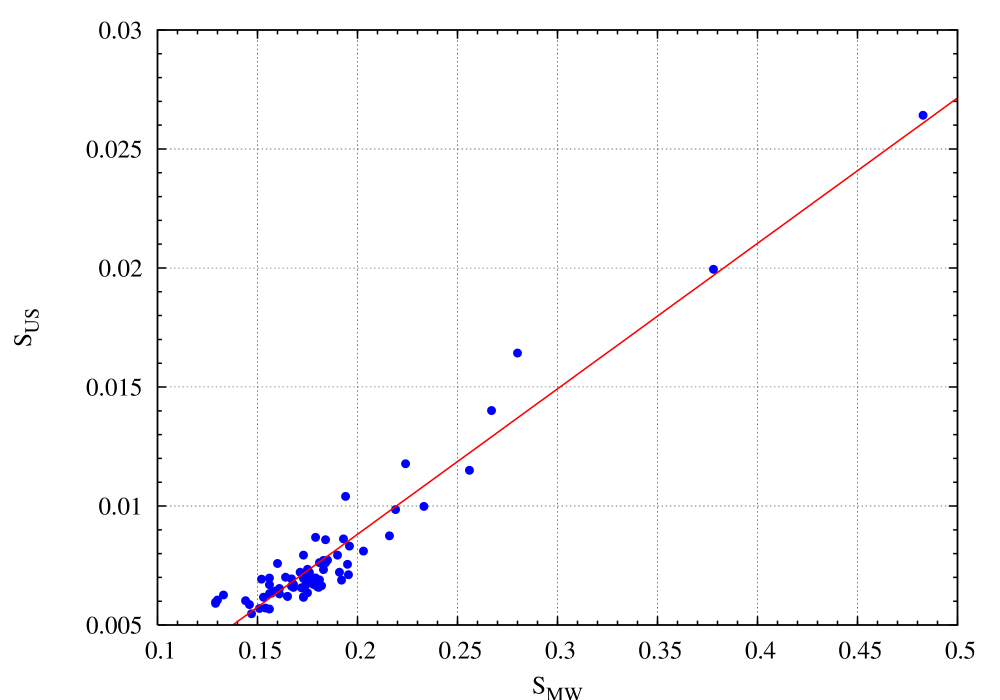
Figure 2: $S_{US}$ compared to the $S_{MW}$ values for a set of calibrators. The solid line is the best least-squared linear fit.

Figure 2 shows our best-fit. The RMS of the residuals of the fit ($\sigma_{fit}$) is $8\times 10^{-4}$. As pointed out by Santos et al. (2000), $\sigma_{fit}$ includes not only uncertainties in the calibration procedure but also intrinsic stellar variation. Eq. 1 can now be used to compute the $S_{MW}$.

The Ca II H and K flux corrected for the photospheric flux ($R^{\prime}_{HK}=R_{HK}-R_{phot}$) is computed using Noyes et al. (1984) prescription. The derived $S_{MW}$ yielded by Eq. 1 and the corrected chromospheric flux $R^{\prime}_{HK}$ are given in Table 1. We note that in this procedure for the OGLE stars and TrES-1 we have used B-V colors that were derived by inverting the B-V vs. (Teff,[Fe/H]) calibration presented in Santos et al. (2004).

No spectra in the CaII-line regions were available for HD149026 and OGLE-TR-132, and no values for the S index are available in the literature for these stars either. For HD209458 we used the value $S_{MW}=0.154$ derived by Wright et al. (2004), the effective temperature and metallicity of Santos et al. (2004) to compute the $R^{\prime}_{HK}$ given in Table 1.

4 Li abundances

Lithium abundances were obtained as in Israelian et al. (2004), from a LTE analysis using a recent version of the radiative transfer code MOOG (Sneden 1973) and a grid of Kurucz (1993) plane-parallel model atmospheres. Equivalent widths (EWs) for the Li line near 6707.8Å (or an upper limit for these) were measured using the IRAF splot routine inside the echelle package. This procedure gives good results since in our spectra the Li line was never strongly blended with any other line in the same spectral region.

The measured EWs (or upper limits for these) were then used to derive the Li abundances. The results are presented in Table 2. We used the stellar parameters listed in Santos et al. (2006), also listed in Table 2 for completeness. For more details on the derivation of Li abundances we refer the reader to Israelian et al. (2004).

For HD209458 we have taken the Li abundance from the study of Israelian et al. (2004). No Li abundances are available for both HD149026 and OGLE-TR-132.

Table 2: Stellar parameters and Li abundances for all known transiting planets. See text for references.

Star	Teff	$\log g$	$\xi_{\mathrm{t}}$	[Fe/H]	Reference	$A(Li)$	Reference
	(K)	(c.g.s)	[km s-1]		Stellar Parameters		$A(Li)$
TrES-1	5226$\pm$38	4.40$\pm$0.10	0.90$\pm$0.05	0.06$\pm$0.05	Santos et al. (2006)	$<0.5$	This paper
OGLE-TR-10	6075$\pm$86	4.54$\pm$0.15	1.45$\pm$0.14	0.28$\pm$0.10	Santos et al. (2006)	2.3$\pm$0.1	This paper
OGLE-TR-56	6119$\pm$62	4.21$\pm$0.19	1.48$\pm$0.11	0.25$\pm$0.08	Santos et al. (2006)	2.7$\pm$0.1	This paper
OGLE-TR-111	5044$\pm$83	4.51$\pm$0.36	1.14$\pm$0.10	0.19$\pm$0.07	Santos et al. (2006)	$<0.5$	This paper
OGLE-TR-113	4804$\pm$106	4.52$\pm$0.26	0.90$\pm$0.18	0.15$\pm$0.10	Santos et al. (2006)	$<0.2$	This paper
OGLE-TR-132	6411$\pm$179	4.86$\pm$0.14	1.46$\pm$0.36	0.43$\pm$0.18	Bouchy et al. (2004)	–
HD149026	6147$\pm$50	4.26$\pm$0.07	–	0.36$\pm$0.05	Sato et al. (2005)	–
HD189733	5050$\pm$50	4.53$\pm$0.14	0.95$\pm$0.07	$-$0.03$\pm$0.04	This paper	$<-0.1$	This paper
HD209458	6117$\pm$26	4.48$\pm$0.08	1.40$\pm$0.06	0.02$\pm$0.03	Santos et al. (2004)	2.7$\pm$0.1	Israelian et al. (2004)

5 Projected rotational velocity

For most of our candidates the projected rotational velocities and the respective errors listed in Table 3 were taken from the literature (Queloz et al. 2000; Pont et al. 2004; Bouchy et al. 2004, 2005a; Sato et al. 2005; Laughlin et al. 2005). For OGLE-TR-10 and OGLE-TR-56 the projected rotational velocities were derived from HARPS spectra using a calibration based on the Cross-Correlation Function width (see e.g. Santos et al. 2002).

Table 3: Estimated $V\sin i$ for the transiting planet host stars studied in this paper.

Star	$V_{rot}$ (km s-1)	Reference
TrES-1	1.08$\pm$0.3	Laughlin et al. (2005)
OGLE-TR-10	7.0$\pm$1.0	HARPS CCF
OGLE-TR-56	3.2$\pm$1.0	HARPS CCF
OGLE-TR-111	$<$5	Pont et al. (2004)
OGLE-TR-113	$<$5	Bouchy et al. (2004)
OGLE-TR-132	$<$5	Bouchy et al. (2004)
HD149026	6.0$\pm$0.5	Sato et al. (2005)
HD189733	3.5$\pm$1.0	Bouchy et al. (2005a)
HD209458	3.75$\pm$1.25	Queloz et al. (2000)

We note that in our case the $V\sin i$ values correspond to the real equatorial rotational velocity, as long as the rotational axis of the star is perpendicular to the orbital plane of the transiting planet. This hypothesis is supported by observations of the Rossiter-McLauglin effect on HD209458 and HD189733 (Queloz et al. 2000; Bouchy et al. 2005a).

6 Age of stars hosting Transiting planets

6.1 Chromospheric ages

The formulae used in deriving stellar ages from chromospheric activity indices are summarized in Wright et al. (2004). A typical projection of the age-activity relation is shown in Fig. 3. The relation between activity and age is steep for young ages and gets flatter for older ages. Additionally, stellar activity follows long-term cycles, and the use of instantaneous chromospheric flux instead of the flux averaged over an entire magnetic cycle leads to an over or under estimation of age depending on which moment of its cycle the star is observed. The classical example being the case of the Sun whose $\log R^{\prime}_{HK}$ varied from -4.75 to -5.10 during the ”Maunder Minimum”, corresponding to ages of 8.0 and 2.2 Gyr, respectively (e.g. Henry et al. 1996).

Pace & Pasquini (2004) have studied empirically the reliability of chromospheric ages by measuring the chromospheric activity level in dwarfs belonging to 5 different open clusters with ages spanning from 0.6 Gyr up to 4.5 Gyr. They found that after a strong decrease in chromospheric activity taking place in solar-type stars between the Hyades and the IC 4651 age (i.e., 0.6 Gyr and 1.7 Gyr), activity remains virtually constant for more than 3 Gyr. Hence an activity-age relation holds up to only about 2.0 Gyr. Therefore, as cautioned by many authors, chromospheric activity indices are good indicators of youth, but cannot yield reliable age estimates beyond $\sim 2-3$ Gyr - as illustrated graphically on Fig.3.

Consequently, since all stars in our sample show low levels of activity, we only derive lower age limits rather than specific age estimates from chromospheric activity. We used the $R^{\prime}_{HK}$ values listed in Table 1 and the calibration of Henry et al. (1996). We calculated the 2-sigma lower limits on the ages by including as far as possible the sources of error on all intermediate steps between the computation of the $S_{US}$ and the final ages and allowed for an intrinsic dispersion of 20% for the activity level of stars with identical mass and age.

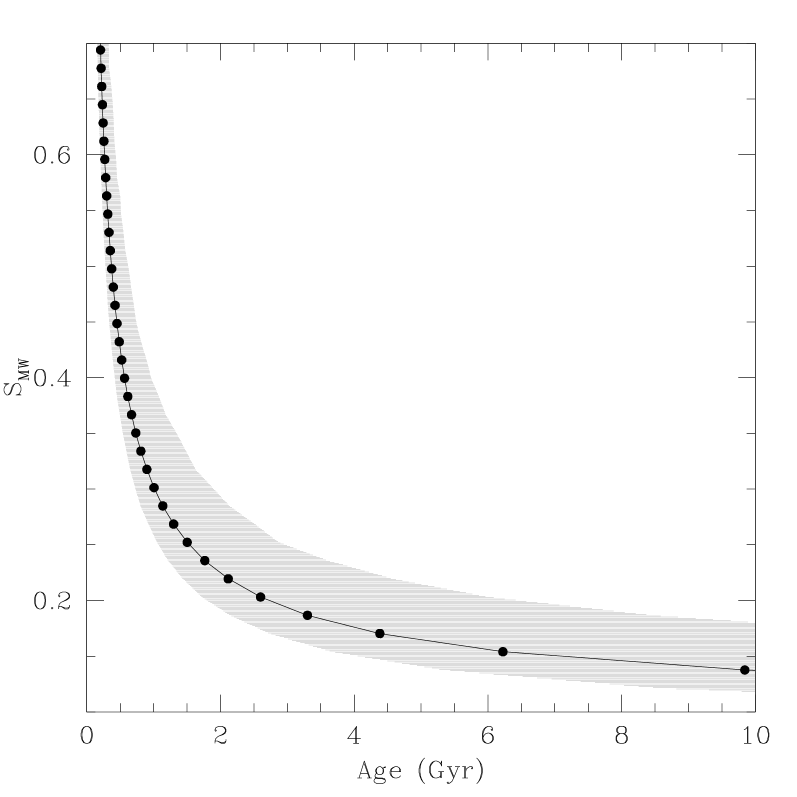
Figure 3: The projection of the age-activity relation for a $B-V=0.63$ star is shown by the circles and solid line. The shaded area around the solid line is the 95% confidence region for the true stellar age computed assuming a 20% variability level on the $S_{US}$. Due to the the flatness of the activity-age calibration it is clearly seen that after 2-3Gyr only a minimum age can be computed by this method.

6.2 Li ages

Li ages given in Table 4 were derived by comparison with abundance curves of Li as a function of effective temperature for clusters of different ages (Jeffries et al. 2002; Sestito & Randich 2005). Due to its fragility, Li is quickly destroyed during the pre-main sequence inside solar-mass stars which are (almost) fully convective at the beginning of their lives. Li depletion also occurs on the main-sequence although its causes are still under strong debate (see review by Deliyannis et al. 2000). For this reason Li is widely used a youth indicator (e.g. Martin 1997).

For stars hotter than 6000 K (i.e., earlier than G), the convective zones are not deep enough to bring Li to warmer regions thus Li is not depleted (with exception of the Li gap; Boesgaard & Tripicco 1986). Hence Li abundance cannot be used as an age indicator. This is the case for OGLE-TR-10 and OGLE-TR-56.

The recent results of Sestito & Randich (2005) seem to indicate that Li-depletion occurs by quick episodes rather than at a monotonic pace. This could imply that Li abundances can only yield lower limits for the ages.

Table 4: Age constraints yielded by each method. The 95%-confidence interval (2-sigma) for the chromospheric age computed using the mean value of $\log R^{\prime}_{HK}$ is shown along with and the age constraint from Li abundances. Whenever available age estimates found in the literature are also given.

Star	ageCaII	ageLi	age	Ref
	$2-\sigma$ lower lim.		other	other
TrES-1	$>$ 1.1	$>$0.6	$2.5\pm 1$	1
OGLE-TR-10	$>$ 1.1	–
OGLE-TR-56	$>$ 2	–	$3\pm 1$	2
OGLE-TR-111	$>$ 1.1	$>$0.6
OGLE-TR-113	$>$ 0.7	$>$0.6
OGLE-TR-132	–	–
HD149026	–	–	$2\pm 0.8$	3
HD189733	$>$ 0.5	$>$0.6
HD209458	$>$ 2	-	4.5	4

1-Sozzetti et al. (2004); 2–Sasselov (2003);
3–Sato et al. (2005); 4–Mazeh et al. (2000)

6.3 $V\sin i$ ages

During the pre-main sequence phase, angular momentum evolution is mainly driven by the magnetic coupling between the star and its disk (e.g. Königl 1991). Due to differences in the disk-locking time-scales, solar type stars arrive on the zero age main sequence presenting a large spread in their rotation rates. From this point on, any angular momentum evolution is dictated by stellar winds whose intensity is itself a function of magnetic activity and rotation (e.g. Kawaler 1988). This creates a regulation mechanism leading to a steady decrease and to the eventual convergence of the rotation rate at about 1Gyr.

Therefore the use the rotation rate as a qualitative age diagnostic is limited. Nevertheless, comparing our $V_{rot}$ given in Table 3 with Figure 2 of Bouvier (1997) we see that despite the large dispersion in the points, the F and G stars with $V_{rot}<5$ km s^-1 are likely to be older than the Hyades ($\sim 600$ Myr), whereas for the cooler stars a $V_{rot}$ of 5 km s^-1 is still compatible with the age of the Pleiades ($\sim 100$ Myr). Similar conclusions can be drawn for OGLE-TR-10 or HD149026 whose $V_{rot}=7$ and 6 km s^-1, respectively, can still be found (although unlikely) among the Pleiades members.

The utility of the $V_{rot}$ values to derive stellar ages is limited, but our results show that globally speaking our sample stars, and in particular those orbited by VHJ, are very unlikely to be younger than the Pleiades (see Figure 2 of Bouvier 1997).

A summary of the age constraints yielded by each method is given in Table 4. As dicussed in Sec. 6.1, any attempt to assign a precise age based on the chromospheric activity is meaningless due to the flatness of the age-activity calibration beyond 2-3Gyr. Therefore, only the lower limit (2-sigma level) from chromospheric activity and the age constraint from Li abundances are given rather than a precise age. Age estimates found in the literature, quoted in Table 4, are consistent with these values.

7 Constraining planetary evaporation rates from stellar ages?

The lower limits given in Table 4 allow us to state that the stars harboring transiting planets studied here are not younger than 0.5 Gyr and for most of them not younger than 1 Gyr at a 2-sigma level. Is this compatible with a very efficient evaporation of these objects?

Efficient evaporation scenarios (Lammer et al. 2003; Lecavelier des Etangs et al. 2004; Baraffe et al. 2004) imply that a fraction of the close-in planets do not survive, at least not as gaseous giants. Therefore those planets seen in present-day transit surveys correspond to the lucky ones that were initially massive enough to escape (so far) evaporation. Our age determinations allow us in principle to constrain the magnitude of the evaporation: stars harboring very close-in planets (and in particular the transiting planets discovered so far) should be on average younger if an efficient evaporation indeed took place. For very large evaporation rates, old stars should have lost their close-in planetary companions, except for the rare ones with very large initial masses.

In order to estimate how the mean age of stars harboring very close-in planets depends on the magnitude of the planetary mass-loss, we proceed as follows. First, it is assumed that the initial masses of the planets are set according to a fixed planetary mass function (see below). Monte-Carlo approach is then used to draw a large number of star-planet systems for which we calculate the fraction of planets that have evaporated away as a function of stellar age and evaporation rate. By re-normalizing this fraction we derive a distribution of the age of stars with planets as a function of the assumed planetary evaporation rate.

The process described above is carried out assuming the following hypotheses:

1. The initial planetary mass function for very-close in planets is the same as for planets observed by radial velocimetry with periods smaller than 365 days (a value chosen to avoid biases for planets with masses $>0.5\rm\,M_{Jup}$, and which is found to affect the results only moderately). The sample used is taken from J. Schneider’s web page (www.obspm.fr/planets) and contains 99 planets.

2. Planets disappear from the sample when their mass becomes smaller than 0.5 M_Jup, either because of a runaway evaporation (Baraffe et al. 2004), or because the presence of a core makes them too small to be detected by the transit method (e.g. Guillot 2005).

3. The stellar formation rate (including stars with planets) has been constant for the past 10 Gyr.

With the present understanding of planet formation and migration, our first hypothesis should be conservative (i.e. allow for higher evaporation rates), as more massive planets are expected to migrate less rapidly and efficiently to become HJ or VHJ planets (Udry et al. 2003; Ida & Lin 2004, e.g.). This is also the case of the third hypothesis, as the progressive enrichment of the Galaxy in metals by stellar nucleosynthesis implies that stars with planets should be on average younger. More detailed studies are needed to address more precisely these points and assess their effect on the results.

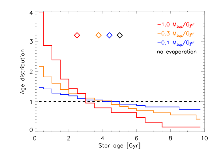
Figure 4: Age distribution of stars with planets, as a function of the planetary evaporation rate. We assume that the unperturbed sample of stars with planets have a uniform age distribution between 0 and 10 Gyr (dashed line). The progressively steeper distributions correspond to evaporation rates of 0.1 (blue), 0.3 (orange) and 1.0 M_Jup/Gyr (red), respectively. The diamonds represent the mean ages of the different distributions.

Figure 4 shows the resulting age distribution of stars with planets for different planetary evaporation rates. For the most extreme case of a 1 M_Jup/Gyr mass loss, the mean of the age distribution is lowered to only 2.5 Gyr. For comparison, according to (Baraffe et al. 2004), the (maximal) evaporation rates derived from an energy-limited approach is almost constant in time and range from 0.1 M_Jup/Gyr (HD209458b, OGLE-TR-10b) to almost 0.7 M_Jup/Gyr (OGLE-TR-132b).

In addition to the age distribution derived in Figure 4, one can now check whether the sample of stars with age determinations derived in this paper is consistent with an energy-limited evaporation scenario. Using again a Monte-Carlo approach and adopting the evaporation rates derived by Baraffe et al. (2004), the distribution of possible ages for each star with transiting planet studied is derived. We then compute the number of times that these ”Monte-Carlo” stellar ages are compatible with the inferred minimal ages, both in the energy-limited evaporation scenario and in the no-evaporation scenario. We found that the latter was between 2 and 3 times more likely, i.e. that the energy-limited evaporation scenario was, in this case, marginally inconsistent with the observations.

Unfortunately, an additional limitation has to be considered, namely, the fact that stars with young ages ($<0.5$ Gyr) are quite active and as such are unlikely to be detected as having a planet (both by the transit method and by radial velocimetry). Due to this further constraint and given the small sample used in this work, we cannot conclude in favor or against the energy-limited evaporation scenario.

8 Conclusions

We have shown that the analysis of high resolution spectra of stars with planets could be used to determine lower limits on their age using Li abundances, the Ca II activity-age relation and from the analysis of the stellar rotational velocity. Applied to six stars known to host transiting giant planets, OGLE-TR-10, 56, 111, 113, TrES-1, and HD189733, we were able to show that none appears to be younger than 1 Gyr at the 2-sigma level.

In principle, this could be used to constrain the amount of mass loss experienced by the planets, since high evaporation rates should yield smaller average ages for the stars with very close-in giant planets. Because of the various uncertainties and small size of the sample studied here, the results remain inconclusive concerning evaporation. However, it highlights the importance of a careful determination of the ages of stars with planets, in particular for the stars harboring very close-in planets (“Pegasids”), but also, as a means of comparison, for stars with planets on orbits with longer-periods.

We hence recommend to pursue the fine determination of the ages of stars with planets, in priority for the transiting planets as they are progressively being detected (for a direct application see Guillot et al. 2006), for non-transiting very close-in giant planets (at less than 0.1 AU from their star), and then for a sample of stars with planets that are orbiting at larger distances.