ZKDR Distance, Angular Size and Phantom Cosmology

Abstract

The influence of mass inhomogeneities on the angular size-redshift test is investigated for a large class of flat cosmological models driven by dark energy plus a cold dark matter component. The results are presented in two steps. First, the mass inhomogeneities are modeled by a generalized Zeldovich-Kantowski-Dyer-Roeder (ZKDR) distance which is characterized by a smoothness parameter $\alpha(z)$ and a power index $\gamma$, and, second, we provide a statistical analysis to angular size data for a large sample of milliarcsecond compact radio sources. By marginalizing over the characteristic angular size $l$, fixing $\Omega_{M}=0.26$ and assuming a Gaussian prior on $\omega$, i.e., $\omega=-1\pm 0.3$, the best fit values are $\omega=-1.03$ and $\alpha=0.9$. By assuming a Gaussian prior on the matter density parameter, i.e., $\Omega_{M}=0.3\pm 0.1$, the best fit model for a phantom cosmology with $\omega=-1.2$ occurs at $\Omega_{M}=0.29$ and $\alpha=0.9$ when we marginalize over the characteristic size of the compact radio sources. The results discussed here suggest that the ZKDR distance can give important corrections to the so-called background tests of dark energy.

1 Introduction

An impressive convergence of recent astronomical observations are suggesting that our world behaves like a spatially flat scenario dominated by cold dark matter (CDM) plus an exotic component endowed with large negative pressure, usually named dark energy (Perlmutter et al. 1998; Efstathiou et al. 2002; Riess et al. 1999, 2004; Allen et al. 2004; Astier et al. 2006; Riess et al. 2007). In the framework of general relativity, besides the cosmological constant, there are several candidates for dark energy, among them: a vacuum decaying energy density, or a time varying $\Lambda(t)$ (Ozer & Taha 1986, 1987; Bertolami 1986; Freese et al. 1987; Carvalho et al. 1992; Lima & Maia 1994; Lima & Trodden 1996; Lima 1996; Torres & Waga 1996; Overduin & Cooperstock 1998; Cunha & Santos 2004; Shapiro et al. 2005, Costa et al. 2007), the so-called “X-matter” (Turner & White 1997; Chiba et al. 1997, Alcaniz & Lima 1999, 2001, Cunha et al. 2003, Da̧browski 2007), a relic scalar field (Peebles & Ratra 1998; Caldwell et al. 1998; Ulam et al. 2004), and a Chaplygin Gas (Kameshchik et al. 2001; Bilíc et al. 2002; Bento et al. 2002; Alcaniz & Lima 2005). Some recent review articles discussing the history, interpretations, as well as, the major difficulties of such candidates have also been published in the last few years (Padmanabhan 2003; Peebles & Ratra 2003; Lima 2004; Turner & Huterer 2007).

In the case of X-matter, for instance, the dark energy component is simply described by an equation of state $p_{x}=\omega\rho_{x}$. The case $\omega=-1$ reduces to the cosmological constant, and together the CDM defines the scenario usually referred to as “cosmic concordance model” ($\Lambda$CDM). The imposition $\omega\geq-1$ is physically motivated by the classical fluid description (Hawking & Ellis 1973). However, as discussed by several authors, such an imposition introduces a strong bias in the parameter determination from observational data. In order to take into account this difficulty, superquintessence or phantom dark energy cosmologies have been recently considered where such a condition is relaxed (Faraoni 2002; Caldwell et al. 2003; Gonzales-Diaz 2003, Santos & Alcaniz 2005, Linder 2007). In contrast to the usual quintessence model, a decoupled phantom component presents an anomalous evolutionary behavior. For instance, the existence of future curvature singularities, a growth of the energy density with the expansion, or even the possibility of a rip-off of the structure of matter at all scales are theoretically expected (see, however, Alcaniz & Lima 2004; Gonzalez-Diaz & Siguenza (2004), de Freitas Pacheco & Hovarth (2007) for a thermodynamic discussion). Although possessing such strange features, the phantom behavior is theoretically allowed by some kinetically scalar field driven cosmology (Chiba et al. 2000), as well as, by brane world models (Shani & Shtanov 2002, 2003, Wu et al. 2007), and, perhaps, more important to the present work, a PhantomCDM cosmology provides a better fit to type Ia Supernovae observations than does the $\Lambda$CDM model(Alam et al. 2003; Choudury & Padmanabhan 2004; Astier et al. 2006). Many others observational and theoretical properties of phantom driven cosmologies have also been successfully confronted to standard results (see, for instance, Alcaniz 2004; Piao & Zhang 2004; Choudury and Padmanabhan 2005; Perivolaropoulos 2005; Nesseris & Perivolaropoulos 2007).

In this context, one of the most important tasks for cosmologists nowadays is to confront different cosmological scenarios driven by cold dark matter (CDM) plus a given dark energy candidate with the available observational data. As widely known, a key quantity for some cosmological tests is the angular distance-redshift relation, $D_{A}(z)$, which for a homogeneous and isotropic background, can readily be derived by using the Einstein field equations for the Friedmann-Robertson-Walker (FRW) geometry. From $D_{A}(z)$ one obtains the expression for the angular diameter $\theta(z)$ (see section 3) which can be compared with the available data for different samples of astronomical objects (Gurvits et al. 1999; Lima & Alcaniz 2000, 2002; Gurvits 2004; Alcaniz & Lima 2005).

Nevertheless, the real Universe is not perfectly homogeneous, with light beams experiencing mass inhomogeneities along their way. Actually, from small to intermediate scales ($\leq 100$Mpc), there is a lot of structure in form of voids, clumps and clusters which is probed by the propagating light. Since the perturbed metric is unknown, an interesting possibility to account for such an effect is to introduce the smoothness parameter $\alpha$ which is a phenomenological representation of the magnification effects experienced by the light beam. From general grounds, one expects a redshift dependence of $\alpha$ since the degree of smoothness for the pressureless matter is supposed to be a time varying quantity (Linder 1988). When $\alpha=1$ (filled beam), the homogeneous FRW case is fully recovered; $\alpha<1$ stands for a defocusing effect while $\alpha=0$ represents a totally clumped universe (empty beam). The distance relation that takes these mass inhomogeneities into account was discussed by Zeldovich (1964) followed by Kantowski (1969), although a clear-cut application for cosmology was given only in 1972 by Dyer & Roeder (many references may be found in the textbook by Schneider, Ehlers & Falco 1992; Kantowski 2003). Many studies involving the ZKDR distances in dark energy models have been published in the literature. Analytical expressions for a general background in the empty beam approximation ($\alpha=0$) were derived by Sereno et al. (2001). By assuming that both dominant components may be clustered they also discussed how the critical redhift, i.e., the value of $z$ for which $D_{A}(z)$ is a maximum (or $\Theta(z)$ minimum), and compared to the homogeneous background results as given by Lima & Alcaniz (2000), and, further discussed by Lewis & Ibata (2002), and Araújo & Stoeger (2007). More recently, Demianski et al. (2003), derived an useful analytical approximate solution for a clumped concordance model ($\Lambda$CDM) valid on the interval $0\leq z\leq 10$. Additional studies on this subject involving time delay (Giovi & Amendola 2001; Lewis & Ibata 2002) gravitational lensing (Kochanek 2002; Kochanek & Schechter 2003) or even accelerated models driven by particle creation (Campos & Souza 2004) have also been considered.

Although carefully investigated in many of their theoretical and observational aspects, an overview in the literature shows that a quantitative analysis on the influence of dark energy in connection with inhomogeneities present in the observed universe still remains to be studied. Recently, the ZKDR distance was applied for the $\theta(z)$ statistics with basis on a $\Lambda$CDM cosmology with constant $\alpha$ (Alcaniz et al. 2004). It was concluded that the best fit model occurs at $\Omega_{M}=0.2$ and $\alpha=0.8$ whether the characteristic angular size $\l$ of the compact radio sources is marginalized.

In this paper, we focus our attention on X-matter cosmologies with special emphasis to phantom models ($\omega<-1$) by taking into account the presence of a clustered cold dark matter. The mass inhomogeneities will be described by the ZKDR distance characterized by a smoothness parameter $\alpha(z)$ which depends on a positive power index $\gamma$. The main objective is to provide a statistical analysis to angular size data from a large sample of milliarcsecond compact radio sources distributed over a wide range of redshifts ($0.011\leq z\leq 4.72$) whose distance is defined by the ZKDR equation. As an extra bonus, it will be shown that a pure CDM model ($\Omega_{M}=1$) is not compatible with these data even for the empty beam approximation ($\alpha=0$). The manuscript is organized as follows. In section 2 we derive the ZKDR equation. We also provide some arguments for a locally nonhomogeneous Universe where the homogeneous contribution of the dark matter obeys the relation $\rho_{h}=\alpha\rho_{o}(\rho_{m}/\rho_{o})^{\gamma}$ where $\gamma$ is a positive number. In section 3 we analyze the constraints on the free parameters $\alpha$, $\gamma$ and $\Omega_{M}$. We end the paper by summarizing the main results in section 4.

2 The Extended ZKDR Equation

Let us now consider a flat FRW geometry ($c=1$)

$$ds^{2}\ =\ dt^{2}\ -\ R^{2}(t)\left(dr^{2}+r^{2}d\theta^{2}+r^{2}\sin^{2}\theta\,d\phi^{2}\right),$$ (1)

where $R(t)$ is the scale factor. Such a spacetime is supported by the pressureless CDM fluid plus a X-matter component of densities $\rho_{M}$ and $\rho_{x}$, respectively. Hence, the total energy momentum tensor, $T^{\mu\nu}={T^{\mu\nu}}_{({M})}+{T^{\mu\nu}}_{({x})}$, can be written as

$$T^{\mu\nu}=[\rho_{M}+(1+\omega)\rho_{x}]U^{\mu}U^{\nu}-\omega\rho_{x}g^{\mu\nu},$$ (2)

where $U^{\mu}=\delta^{\mu}_{o}$ is the hydrodynamics 4-velocity of the comoving volume elements. In this framework, the Einstein Field Equations (EFE)

$$G^{\mu\nu}\equiv R^{\mu\nu}-\frac{1}{2}g^{\mu\nu}R=8\pi GT^{\mu\nu},$$ (3)

take the following form:

$$({\dot{R}\over R})^{2}=H_{o}^{2}\left[\Omega_{\rm{M}}({R_{o}\over R})^{3}+\Omega_{x}({R_{o}\over R})^{3(1+\omega)}\right],$$ (4)

$${\ddot{R}\over R}=-{1\over 2}H_{o}^{2}\left[\Omega_{\rm{M}}({R_{o}\over R})^{3}+(3\omega+1)\Omega_{x}({R_{o}\over R})^{3(1+\omega)}\right],$$ (5)

where an overdot denotes derivative with respect to time and $H_{o}=100h{\rm{Kms^{-1}Mpc^{-1}}}$ is the Hubble parameter. By the flat condition, $\Omega_{x}=1-\Omega_{\rm{M}}$, is the present day dark energy density parameter. As one may check from (2)-(5), the case $\omega=-1$ describes effectively the favored “cosmic concordance model” ($\Lambda$CDM).

On the other hand, in the framework of a comformally flat FRW metric, the optical scalar equation in the geometric optics approximation reads (Optical shear neglected)

$${\sqrt{A}}^{\prime\prime}+\frac{1}{2}R_{\mu\nu}k^{\mu}k^{\nu}\sqrt{A}=0,$$ (6)

where $A$ is the beam cross sectional area, plicas means derivative with respect to the affine parameter describing the null geodesics, and $k^{\mu}$ is a 4-vector tangent to the photon trajectory whose divergence determines the optical scalar expansion (Linder 1988; Giovi & Amendola 2001; Demianski et al. 2000, Sereno et al. 2001). The circular frequency of the light ray as seen by the observer with 4-velocity $U^{\alpha}$ is $\omega=U^{\alpha}k_{\alpha}$, while the angular diameter distance, $D_{A}$, is proportional to $\sqrt{A}$ (Schneider, Ehlers & Falco 1992).

As widely known, there is no an acceptable averaging procedure for smoothing out local inhomogeneities. After Dyer & Roeder (1972), it is usual to introduce a phenomenological parameter, $\alpha(z)=1-{\rho_{cl}\over<\rho_{m}>}$, called the “smoothness” parameter. For each value of $z$, such a parameter quantifies the portion of matter in clumps ($\rho_{cl}$) relative to the amount of background matter which is uniformly distributed ($\rho_{m}$). As a matter of fact, such authors examined only the case for constant $\alpha$, however, the basic consequence of the structure formation process is that it must be a function of the redshift. Combining equations (2), (3) and (6), after a straightforward but lengthy algebra one finds that the angular diameter distance, $D_{A}(z)$, obeys the following differential equation

$$\left(1+z\right)^{2}{\cal{F}}\frac{d^{2}D_{A}}{dz^{2}}+\left(1+z\right){\cal{G}}\frac{dD_{A}}{dz}+{\cal{H}}D_{A}=0,$$ (7)

which satisfies the boundary conditions:

$$\left\{\begin{array}[]{c}D_{A}\left(0\right)=0,\\ \\ \frac{dD_{A}}{dz}|_{0}=1.\end{array}\right.$$ (8)

The functions ${\cal{F}}$, ${\cal{G}}$ and ${\cal{H}}$ in equation (7) read

$${\cal{F}} = \Omega_{M}(1+z)^{3}+(1-\Omega_{M})(1+z)^{3(\omega+1)}$$

$${\cal{G}} = \frac{7}{2}\Omega_{M}(1+z)^{3}+\frac{3\omega+7}{2}(1-\Omega_{M})(1+z)^{3(\omega+1)}$$

$${\cal{H}} = \frac{3\alpha(z)}{2}\Omega_{M}(1+z)^{3}+$$ (9)

$$+\frac{3(\omega+1)}{2}(1-\Omega_{M})(1+z)^{3(\omega+1)}.$$

The smoothness parameter $\alpha(z)$, appearing in the expression of ${\cal{H}}$, assumes the form below (see Appendix A for a detailed discussion)

$$\alpha(z)=\frac{\beta_{o}(1+z)^{3\gamma}}{1+\beta_{o}(1+z)^{3\gamma}},$$ (10)

where $\beta_{o}$ and $\gamma$ are constants. Note that the fraction $\alpha_{o}=\beta_{o}/(1+\beta_{o})$ is the present day value of $\alpha(z)$. In Fig. 1 we show the general behavior of $\alpha(z)$ for some selected values of $\beta_{o}$ and $\gamma$.

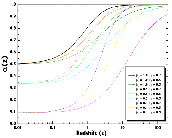
Figure 1: The smoothness parameter as a function of the redshift for some selected values of $\beta_{o}$ and $\gamma$. All curves approach the filled beam result ($\alpha=1$) at high redshifts regardless of the values of $\beta_{o}$ and $\gamma$. Note that $\beta_{o}$ determines $\alpha_{o}=\alpha(z=0)$. For a given $\beta_{o}$ the curves starts at the same point but the rate approaching unit (filled beam) depends on the $\gamma$ parameter.

At this point, it is interesting to compare Eq. (7) together the subsidiary definitions (8)-(10) with other treatments appearing in the literature. For $\gamma=0$ (constant $\alpha$) and $\omega=-1$ ($\Lambda$CDM) it reduces to Eq. (2) as given by Alcaniz et al. (2004). In fact, for $\omega=-1$ the function ${\cal{H}}$ is given by ${\cal{H}}=\frac{3\alpha}{2}\Omega_{M}(1+z)^{3}$. A more general expression for $\Lambda$CDM model (by including the curvature term) has been derived by Demianski et al. (2004). As one may check, by identifying $\omega\equiv m/3-1$, our Eq. (7) is exactly Eq.(10) presented by Giovi & Amendola (2001) in their time delay studies (see also Eq. (2) of Sereno et al. (2002)). It is worth notice that in this paper the $\alpha$ parameter is greater than unity. This means that the light rays are demagnified along the path (for $\alpha<1$ the light rays are magnified). In addition, the $\alpha$ parameter may also depend on the direction along the line of sight (for a discussion of such effects see Wang 1999, Sereno et al. 2002).

Let us now discuss the integration of the ZKDR equation with emphasis in the so-called phantom dark energy model ($\omega<-1$). In what follows, assuming that $\omega$ is a constant, we have applied for all graphics a simple Runge-Kutta scheme (see, for instance, the rksuite package from www.netlib.org).

In Figure 2 one can see how the equation of state parameter, $\omega$, affects the angular diameter distance. For fixed values of $\Omega_{M}=0.3$, $\beta_{o}=0.5$ and $\gamma=0$, all the distances increase with the redshift when $\omega$ diminishes and enters in the phantom regime ($\omega<-1$). For comparison we have also plotted the case for $\Lambda$CDM cosmology ($\omega=-1$).

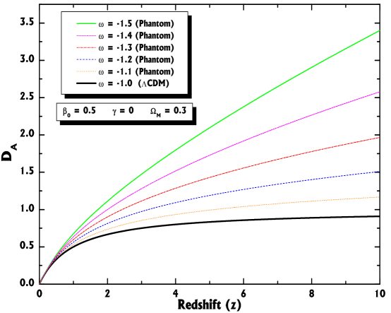
Figure 2: Angular diameter distance for a flat FRW phantom cosmology. The curves display the effect of the equation of state parameter for $\beta_{o}=0.5$ and $\gamma=0$. The thick curve corresponds to the $\Lambda$CDM model. Note that for a given redshift, the distances always increase for $\omega$ beyond the phantom divide line ($\omega<-1$).

In Fig. 3 we show the effect of the $\gamma$ parameter on the angular diameter distance for a specific phantom cosmology with $\omega=-1.3$, as requested by some recent analyzes of Supernovae data (Riess 2004, Perivolopoulus 2004). For this plot we have considered $\beta_{o}=0.5$. As shown in Appendix A, $\beta_{o}=(\rho_{h}/\rho_{cl})_{z=0}$, is the present ratio between the homogeneous ($\rho_{h}$) and the clumped ($\rho_{cl}$) fractions. It was fixed in such a way that $\alpha_{o}$ assumes the value $0.33$. Until redshifts of the order of 2, the distance grows for smaller values of $\gamma$, and after that, it decreases following nearly the same behavior.

In Fig. 4 we display the influence of the $\beta_{o}$ parameter on the angular diameter distance for two distinct sets of $\gamma$ values. The cosmological framework is defined $\Omega_{M}=0.3$ and the same equation of state parameter $\omega=-1.3$ (phantom cosmology). For each branch (a subset of 3 curves with fixed $\gamma$) the distance increases for smaller values of $\beta_{o}$, as should be expected.

3 ZKDR distance and Angular Size Statistics

As we have seen, in order to apply the angular diameter distance to a more realistic description of the universe it is necessary to take into account local inhomogeneities in the distribution of matter. Similarly, such a statement remains true for any cosmological test involving angular diameter distances, as for instance, measurements of angular size, $\theta(z)$, of distant objects. Thus, instead of the standard FRW homogeneous diameter distance one must consider the solutions of the ZKDR equation.

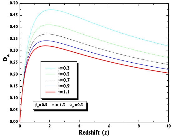
Figure 3: Effects of the $\gamma$ parameter on the angular diameter distance. For all curves we fixed $\omega=-1.3$, $\beta_{o}=0.5$ and $\Omega_{M}=0.3$. Note that the distances increase for smaller values of $\gamma$.

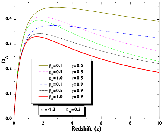
Figure 4: Influence of the $\beta_{o}$ parameter on the angular diameter distance for $\Omega_{M}=0.3$ and $\omega=-1.3$. The curves are separated in two sets corresponding to the values of $\gamma=0.5,0.9$ as indicated in the box. As expected, both sets present the same behavior at low redshifts.

Here we are concerned with angular diameters of light sources described as rigid rods and not isophotal diameters. In the FRW metric, the angular size of a light source of proper length ${\l}$ (assumed free of evolutionary effects) and located at redshift $z$ can be written as

$$\theta(z)=\frac{\ell}{{D_{A}}(z)},$$ (11)

where $\ell=100{\l}$h is the angular size scale expressed in milliarcsecond (mas) while ${\l}$ is measured in parsecs for compact radio sources (see below).

Let us now discuss the constraints from angular size measurements of high $z$ objects on the cosmological parameters. The present analysis is based on the angular size data for milliarcsecond compact radio sources compiled by Gurvits et al. (1999). This sample is composed by 145 sources at low and high redshifts ($0.011\leq z\leq 4.72$) distributed into 12 bins with 12-13 sources per bin (for more details see Gurvits et al. 1999). In Figure 5 we show the binned data of the median angular size plotted as a function of redshift $z$ to the case with $\gamma=0$ and some selected values of $\Omega_{M}$ and $\alpha_{o}=\beta_{o}/(1-\beta_{o})$ = constant. As can be seen there, for a given value of $\Omega_{M}$ the corresponding curve is slightly modified for different values of the smoothness parameter $\alpha$.

Now, in order to constrain the cosmic parameters, we first fix the central value of the Hubble parameter obtained by the HST key project $H_{o}=72\pm 8$ ${\rm{km.s^{-1}.Mpc^{-1}}}$ (Freedman et al. 2001). Note that this value is greater that the recent determination by Sandage and collaborators (see astro-ph/0603647), and it is in accordance with the 3 years release of the WMAP team. Following standard lines, the confidence regions are constructed through a $\chi^{2}$ minimization

$$\chi^{2}(l,\omega,\alpha)=\sum_{i=1}^{12}{\frac{\left[\theta(z_{i},\l,\omega,\alpha)-\theta_{oi}\right]^{2}}{\sigma_{i}^{2}}},$$ (12)

where $\theta(z_{i}$, $\l$, $\omega$, $\alpha)$ is defined from Eq. (7) and $\theta_{oi}$ are the observed values of the angular size with errors $\sigma_{i}$ of the $i$th bin in the sample. The confidence regions are defined by the conventional two-parameters $\chi^{2}$ levels. In this analysis, the intrinsic length $\l$, is considered a kind of “nuisance” parameter, and, as such, we have also marginalized over it.

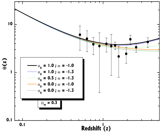
Figure 5: Angular size versus redshift according to the ZKDR distance. Curves for $\Omega_{M}=0.3$, $\gamma=0$ and different values of $\omega$ are shown. The data points correspond to 145 compact radio sources binned into 12 bins (Gurvits et al. 1999). For comparison the filled beam $\Lambda$CDM has been included.

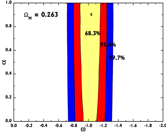
Figure 6: Confidence regions in the $\omega-\alpha$ plane according to the sample of angular size data by Gurvits et al. (1999) and fixed $\Omega_{M}=0.263$ as shown in panel. The confidence levels of the contours are indicated. The point “x” marks the best fit values, $\omega=-1.03$ and $\alpha=0.90$.

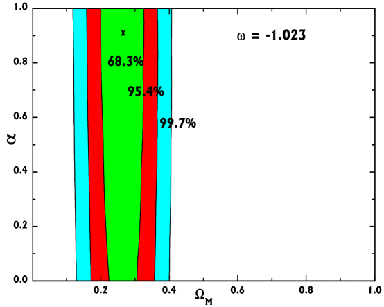
Figure 7: Confidence regions in the $\Omega_{M}-\alpha$ plane according to the sample of angular size data by Gurvits et al. (1999). For a phantom cosmology with $\omega=-1.2$, the confidence levels of the contours are indicated. As in Fig. 6, the “x” also points to the best fit values shown in the panel.

In Fig. 6 we show confidence regions in the $\omega-\alpha$ plane fixing $\Omega_{M}=0.263$, and assuming a Gaussian prior on the $\omega$ parameter, i.e., $\omega=-1\pm 0.3$ (in order to accelerate the universe). The “$\times$” indicates the best fit model that occurs at $\omega=-1.03$ and $\alpha\simeq 0.9$.

In Fig. 7 the confidence regions are shown in the $\Omega_{M}-\alpha$ plane. We have now assumed a Gaussian prior on $\Omega_{M}$, i.e., $\Omega_{M}=0.3\pm 0.1$ from the large scale structure. From Figs. 6 and 7, it is also perceptible that while the parameters $\omega$ and $\Omega_{M}$ are strongly restricted, the entire interval of $\alpha$ is still allowed. This shows the impossibility of tightly constraining the smoothness parameter $\alpha$ with the current angular size data. This result is in good agreement with the one found by Lima & Alcaniz (2002) where the same data set were used to investigate constraints on quintessence scenarios in homogeneous background, and is also in line with the one obtained by Barber et al. (2000) who argued in favor of $\alpha_{o}=\alpha(z=0)$ near unity (see also Alcaniz, Lima & Silva 2004 for constraints on the $\Lambda$CDM model).

4 Summary and Concluding Remarks

All cosmological distances must be notably modified whether the space-time is filled by a smooth dark energy component with negative pressure plus a clustered dark matter. Here we have addressed the question of how the angular diameter distance of extragalactic objects are modified by assuming a slightly inhomogeneous universe. The present treatment complements our previous studies (Alcaniz & Lima 2000, 2002) by considering that the inhomogeneities can be described by the Zeldovich-Kantowski-Dyer-Roeder distance (in this connection see also, Giovi & Amendola 2001; Lewis & Ibata 2002; Sereno et al. 2001; Demianski et al. 2003). The dark energy component was described by the equation of state $p_{x}=\omega\rho_{x}$. A special emphasis was given to the case of phantom cosmology ($\omega<-1$) when the dominant energy condition is violated. The effects of the local clustered distribution of dark matter have been described by the “smoothness” phenomenological parameter $\alpha(z)$, and a simple argument for its functional redshift dependence was given in the Appendix A (see also Figure 1).

The influence of the dark energy component was quantified by considering the angular diameters for sample of milliarcsecond radio sources (Fig. 5) as described by Gurvits et al. (1999). By marginalizing over the characteristic angular size $l$ and assuming a Gaussian prior on the matter density parameter, i.e., $\Omega_{M}=0.263\pm 0.07$(stat) $\pm 0.032$ (sys), the best fit model occurs at $\omega=-1.03$ and $\alpha=0.9$. This phantom model coincides with the central value recently determined by the Supernova Legacy Survey (Astier et. al. 2006). On the other hand, fixing $\omega=-1.3$ and assuming a Gaussian prior for $\Omega_{M}$, that is, $\Omega_{M}=0.3\pm 0.1$, we obtained the best fit values ($\Omega_{M}=0.29$, $\alpha=0.9$).

Finally, it should be stressed that measurements from the angular size combined with the ZKDR approach may provide an important and more rigorous cosmological test in the near future. However, it is necessary a statistical study for determining the intrinsic length of the compact radio sources in order to improve the present results.

Appendix A On the redshift dependence of $\alpha(z)$

In this Appendix we discuss the functional redshift dependence of the smoothness parameter, $\alpha(z)$, adopted in this work. By definition

$$\alpha(z)=1-\frac{\rho_{cl}(z)}{\rho_{m}(z)},$$ (A1)

where $\rho_{cl}$ denotes the clumped fraction of the total matter density, $\rho_{m}$, present in the considered FRW type Universe. This means that the ratio between the homogeneous ($\rho_{h}$) and the clumped fraction can be written as $\rho_{h}/\rho_{cl}=\alpha(z)/1-\alpha(z)$. How this ratio depends on the redshift? In this concern, we first remember that $\alpha(z)$ lies on the interval [0,1]. Secondly, in virtue of the structure formation process, one expects that the degree of homogeneity must increase for higher redshifts, or equivalently, the clumped fraction should be asymptotically vanishing at early times, say, for $z\geq 100$. This means that $\alpha(z)\rightarrow 1$ at high z. At present, ($z=0$), this fraction may have an intermediate value, say, $\beta_{o}$. In addition, it is also natural to suppose that the redshift dependence of the total matter density, $\rho_{m}$, must play an important role in the evolution of their fractions. In this way, for the sake of generality, we will assume a power law

$$\frac{\rho_{h}}{\rho_{cl}}\equiv\frac{\alpha(z)}{1-\alpha(z)}=\beta_{o}(\frac{\rho_{m}}{\rho_{o}})^{\gamma}.$$ (A2)

where $\beta_{o}=(\rho_{h}/\rho_{cl})_{z=0}$ and $\gamma$ are dimensionless numbers. Finally, inserting $\rho_{m}(z)$, and solving for $\alpha(z)$ we obtain:

$$\alpha(z)=\frac{\beta_{o}(1+z)^{3\gamma}}{1+\beta_{o}(1+z)^{3\gamma}},$$ (A3)

which is the expression adopted in this work (see Eq. (9)).

As one may check, for positive values of $\gamma$, the smoothness function (A.3) has all the physically desirable properties above discussed. In particular, the limit for high values of $z$ does not depend on the values of $\beta_{o}$ and $\gamma$ (both of the order of unity). Note also that if the clumped and homogeneous portions are contributing equally at present ($\beta_{o}=1$), we see that $\alpha(z=0)=1/2$ regardless of the value of $\gamma$. Figure 1 display the general behavior of $\alpha(z)$ with the redshift for different choices of $\beta_{o}$ and $\gamma$. The above functional dependence should be compared with the other ones discussed in the literature (Linder 1988, 1998; Campos & de Souza 2004 and Refs. therein). One of the most interesting features of (A.3) is that its validity is not restricted to a given redshift interval.

References

- (1) Alam, A., Sahni, V. & Starobinsky, A. A. 2004, JCAP 0406, 008
- (2) Alcaniz, J. S. & Lima, J. A. S. 1999, ApJ 521, L87; ibdem 2001, ApJ 550, L133
- (3) Alcaniz, J. S. 2004, PRD 69, 083521
- (4) Alcaniz, J. S. & Lima, J. A. S. 2005, ApJ 618, 16
- (5) Alcaniz, J. S., Lima, J. A. S. & Silva, R. 2004, IJMPD 13, 1309
- (6) Araújo M. E. & Stoeger W. R. 2007, arXiv:0705.1846
- (7) Allen, S. W. et al. 2004, MNRAS 353, 457
- (8) Asada, H. 1998, ApJ 501, 473
- (9) Astier, P. et al. 2006, A&A 447, 31
- (10) Bertolami, O. 1986, N. Cim. B 93, 36
- (11) Barber, A. J. et al. 2000, MNRAS 319, 267
- (12) Bento, M. C., Bertolami, O. & Sen, A. A. 2002, PRD 66, 043507
- (13) Bilíc, N., Tupper, G. B., & Viollier, R. D. 2002, Phys. Lett. B 535, 17
- (14) Boisseau, B., Esposito-Farese, G., Polarski, D. & Starobinski, A. 2000, Phys. Rev. Lett. 85, 2236
- (15) Caldwell, R. R., Steinhardt, P. J. 1998, PRD 57, 6057
- (16) Caldwell, R. R., Kamionkowski, M., Weinberg, N. N. 2003, PRL 91, 071301
- (17) Campos, M. & de Souza, J. A. 2004, A&A 422, 401
- (18) Carvalho, J. C., Lima, J. A. S. & Waga, I. 1992, PRD 46, 2404
- (19) Chiba, T., Sugiyama, N. & Nakamura, T. 1997, MNRAS 289, L5
- (20) Chiba, T., Okabe, T., Yamaguchi, M. 2000, PRD 62, 023511
- (21) Choudhury, T. R., Padmanabhan, T. 2004, PRD 69, 064033
- (22) Choudhury, T. R., Padmanabhan, T. 2005, ASP Conference Series 342, 497; 2005, A&A 429, 807
- (23) Costa, F. E. M., Alcaniz J. S. & Maia J. M. F. 2007, arXiv:0708.3800
- (24) Covone, G., Sereno, M. & de Ritis, R. 2005, MNRAS 357, 773
- (25) Cunha, J. V., Santos, R. C. 2004, IJMPD 13, 1321
- (26) Da̧browski, M. P. 2007, arXiv:gr-qc/0701057
- (27) de Freitas Pacheco, J. A., Hovarth, J. 2007, arXiv:0709.1240
- (28) Demianski, M., de Ritis, R., Marino, A. A., Piedipalumbo, E. 2003, A&A 411, 33
- (29) Dyer, C. C. & Roeder, R. C. 1972, ApJ 174, L115; 1972, ApJ 180, L31
- (30) Efstathiou, G. et. al. 2002, MNRAS 330, L29
- (31) Faraoni, V. 2002, IJMP D 11, 471
- (32) Freedman, W. et al. 2001, ApJ 553, 47
- (33) Freese, K., Adams, F. C., Frieman, J. A., & Mottola, E. 1987, Nucl. Phys. B 287, 797
- (34) Giovi, F. & Amendola, L. 2001, MNRAS 325, 1097
- (35) Gonz alez-Diaz, P.F. and Siguenza, C.L., 2004, Nucl. Phys. B697, 363
- (36) Gurvits, L. I. 2004, New Astron. Rev. 48, 1511
- (37) Gurvits, L. I., Kellermann, K. I. & Frey, S. 1999 A&A 342, 378
- (38) Hawking, S. W. & Ellis, G. F. R. 1973, The large scale structure of space-time, Cambridge UP, Cambridge
- (39) Kamenshchik, A., Moschell, U., & Pasquier, V. 2001, Phys. Lett. B 511, 265
- (40) Kantowski, R. 1969, ApJ 155, 89
- (41) Kantowski, R. 2003, PRD 68, 123516
- (42) Kochanek, C. S. 2002, ApJ 578, 25
- (43) Kochanek, C. S. & Schechter, P. L. 2003, astro-ph/0306040
- (44) Lewis, G. F. & Ibata, R. A. 2002, MNRAS 337, 26
- (45) Lima, J. A. S., Cunha, J. V. & Alcaniz, J. S. 2003, PRD 68, 023510, astro-ph/0303388
- (46) Lima, J. A. S. & Maia, J. M. F. 1994, PRD 49, 5597
- (47) Lima, J. A. S. & Trodden, M. 1996, PRD 53, 4280
- (48) Lima, J. A. S. 2004, Braz. Jour. Phys. 34, 194 astro-ph/0402109
- (49) Lima, J. A. S. & Alcaniz, J. S. 2000, A&A 357, 393; ibdem 2000 Gen. Relativ. Gravit. 32, 1851
- (50) Lima, J. A. S. & Alcaniz, J. S. 2002, ApJ 566, 15
- (51) Lima, J. A. S. & Alcaniz, J. S. 2004, Phys. Lett. B 600, 191, astro-ph/0402265
- (52) Linder, E. V. 1988, A&A 206, 190
- (53) Linder, E. V. 1998, ApJ 497, 28
- (54) Linder, E. V. 2007, arXiv:0704.2064
- (55) Nesseris, S., Perivolaropoulos, L. 2004, PRD 70, 043531
- (56) Overduin, F. M. & Cooperstock, F. I. 1998, PRD 58, 043506
- (57) Özer, M. & Taha, M. O. 1986, Phys. Lett. B 171, 363; ibdem; 1987, Nucl. Phys. B 287, 776
- (58) Padmanabhan, T. 2003, Phys. Rept. 380, 235
- (59) Padmanabhan, T. & Choudhury, T. R. 2003, MNRAS, 344, 823
- (60) Peebles, P. J. E. & Ratra, B. 2003, Rev. Mod. Phys. 75, 559
- (61) Perlmutter, S. et al. 1998, Nature 391, 51
- (62) Perivolaropoulos, L. 2005, PRD 71, 063503
- (63) Nesseris, S. & Perivolaropoulos, L. 2007, JCAP 0701, 018
- (64) Perrotta, F. et al. 2002, MNRAS 329, 445
- (65) Piao, Yun-Song; Zhang, Yuan-Zhong 2004, PRD 70, 063513
- (66) Riess, A. G. et al. 1998, AJ 116, 1009
- (67) Riess, A. G. et al. 2004, ApJ 607, 665
- (68) Riess A. G. et al., 2007, ApJ 659, 98
- (69) Sandage, A. et al. 2006, astro-ph/0603647
- (70) Santos, J. & Alcaniz, J. S. 2005, Phys. Lett. B 619, 11
- (71) Schneider, P., Ehlers, J. & Falco, E. E. 1992, Gravitational lenses, Springer - Verlag, Berlin
- (72) Sereno, M., Covone, G., Piedipalumbo, E., de Ritis, R. 2001, MNRAS 327, 517
- (73) Sereno, M., Piedipalumbo, E. & Sazhin, M. V. 2002, MNRAS 335, 1061
- (74) Shani, V. & Shtanov, Y. 2002, IJMP A 11, 1
- (75) Shani, V. & Shtanov, Y., 2003 JCAP 0311, 014, astro-ph/0202346
- (76) Turner M. S., Huterer D., 2007, arXiv:0706.2186
- (77) Torres, L. F. B. & Waga, I 1996, MNRAS, 279, 712
- (78) Turner, M. S., & White, M. 1997, PRD 56, R4439
- (79) Wang, Y. 1999, ApJ. J. 525, 651
- (80) Wu S.-F., Chatrabhuti A., Yang G.-H., Zhang P-M 2007, arXiv:0708.1038
- (81) Zeldovich, Ya. B. 1964, Sov. Astron. 8, 13