VLT-UVES abundance analysis of four giants in NGC 6553

Abstract

Context. Metal-rich globular clusters trace the formation of bulges. Abundance ratios in the metal-rich globular clusters such as NGC 6553 can constrain the formation timescale of the Galactic bulge.

Aims. The purpose of this study is determine the metallicity and elemental ratios in individual stars of the metal-rich bulge globular cluster NGC 6553.

Methods. A detailed abundance analysis of four giants in NGC 6553 is carried out, based on optical high-resolution échelle spectra obtained with UVES at the ESO VLT-UT2 Kueyen telescope.

Results. A metallicity [Fe/H]= $-$0.20 dex is derived, together with $\alpha$-element enhancement of Mg and Si ([Mg/Fe]=+0.28, [Si/Fe]=+0.21), solar Ca and Ti ([Ca/Fe]=+0.05, [Ti/Fe]=$-$0.01), and a mild enhancement of the r-process element Eu with [Eu/Fe] = $+$0.10. A mean heliocentric radial velocity of $-$1.86 km s^-1 is measured. We compare our results with previous investigations of the cluster.

1 Introduction

Metal-rich red globular clusters trace the build up of bulges and possibly of disks (Brodie & Strader 2006). They may be formed during an early collapse (Forbes et al. 1997; Côté et al. 1998); otherwise, in hierarchical scenarios the metal-rich globular clusters would be direct probes of the merging events and assembly of the host galaxy (Ashman & Zepf 1992; Beasley et al. 2002; Bekki 2005). Another possibility is bulge formation via the secular evolution of a bar (Kormendy & Kennicutt 2004). Their detailed study should help constrain models of globular cluster formation in the early Galaxy.

Several studies have tried to infer some of the main properties of NGC 6553. Minniti (1995) argues that the metal-rich globular clusters in the inner spheroid are associated with the galactic bulge. Zoccali et al. (2001, 2003) determined the proper motion of NGC 6553 and conclude that this cluster follows the mean rotation of both disk and bulge stars, whereas Dinescu et al. (2003) conclude that this cluster belongs to a rotationally supported disk system. Ortolani et al. (1995) show that NGC 6528 and NGC 6553 are old. Another tool for better understanding the origin of these metal-rich clusters is the chemical composition of individual member stars.

The globular clusters in the bulge NGC 6553, NGC 6528, NGC 6440, and Liller 1 are among the most metal-rich clusters in the Galaxy (Barbuy et al. 1998). Ortolani et al. (1990) point out the turnover and fainter red giant branch (RGB) of NGC 6553, relative to less metal-rich clusters, indicating that TiO blanketing should contribute to the RGB behaviour, being in itself an indicator of high metallicity. These metal-rich clusters constitute the only available calibrators for metallicity and abundance ratio measurement methods based on low-resolution spectra and/or population synthesis of composite spectra of star clusters and galaxies.

NGC 6553 is the most studied bulge globular cluster, and yet only few stars were analysed at high resolution. The CCD analyses were carried out for one giant by Barbuy et al. (1992) and two giants by Barbuy et al. (1999) at moderate resolution (R$\sim$20 000), five red horizontal branch stars by Cohen et al. (1999) at high resolution (R$\sim$34 000), whereas in the H band two giants were analysed by Origlia et al. (2002) at moderate resolution (R$\sim$25 000) and five giants by Meléndez et al. (2003) at high resolution (R$\sim$50 000). Carretta et al. (2001) revised the Cohen et al. (1999) analysis. These previous results gave metallicities in the range $-$0.55 $<$ [Fe/H] $<$ $-$0.06.

We present the analysis of four giants based on high-resolution (R = 55 000) spectra obtained at the VLT-UT2 Kueyen telescope equipped with the UVES spectrograph. These are the highest resolution observations available for stars in this cluster. Since we are dealing with cool metal-rich giants, high-resolution spectroscopy is mandatory.

The observations and radial velocity derivation are described in Sect. 2. In Sect. 3 the stellar parameters are presented, the abundances are derived in Sect. 4, the results are discussed in Sect. 5, and a summary is given in Sect. 6.

2 Observations

2.1 Imaging

NGC 6553 ($\alpha_{\rm J2000}$ = 18^h09^m17.6^s, $\delta_{\rm J2000}$ = $-$25^o54^′31^′′, l = 5.25^∘, b = $-$3.03^∘) is located at low galactic latitude and is projected in the direction of the Galactic centre with X = +5.9kpc, Y = +0.5kpc, and Z = $-$ 0.3kpc. It has a relatively low extinction of E_B-V= 0.70 mag (Guarnieri et al. 1998) and a high luminosity of M_V = $-$7.77 mag, (Harris 1996).

The $BVI$ observations of NGC 6553 were obtained in June 2002 with the wide-field imager (WFI) at the 2.2m ESO-MPI telescope (La Silla, Chile). The data were obtained within our program dedicated to surveying the Galactic globular clusters with the WFI (Zoccali et al. 2001). The $J$$H$$K_{S}$ colours are from the 2MASS Atlas (Cutri et al. 2003). No J,H,K photometry for the sample stars II-64 and 267092 are currently available.

In Fig. 1 we show the location of target sample stars on the colour-diagram magnitude (CMD) of NGC 6553 using Hubble Space Telescope (HST) data (Ortolani et al. 1995), with three stars located at the horizontal branch (HB) level and one of them at the tip of the RGB. The identifications follow the notation given in Hartwick (1975) and in the WFI data obtained with the ESO-MPI telescope.

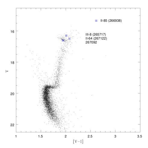
Figure 1: $V$ vs. $V-I$ CMD of NGC 6553 with the target stars indicated.

2.2 High-resolution spectra

High-resolution spectra of four giants in NGC 6553, in the wavelength range $\lambda\lambda$ 4800-6800 Å, were obtained with the UVES spectrograph (Dekker et al. 2000) at the ESO VLT-UT2 Kueyen telescope. The red portion of the spectrum (5800-6800 Å) was obtained with the MIT backside-illuminated ESO CCD # 20, of 4096x2048 pixels, and pixel size 15x15$\mu$m. The blue portion of the spectrum (4800-5800 Å) used ESO Marlene EEV CCD-44, backside illuminated, 4102x2048 pixels, and pixel size 15x15$\mu$m. With the UVES standard setup 580, the resolving power (R=$\lambda/\Delta\lambda$) is R $\simeq$ 55 000 for a slit of 0.8”. Typical signal-to-noise (S/N) ratios for the spectra were obtained considering average values at different wavelengths. The pixel scale is 0.0147 Å/pix. Spectra of rapidly rotating hot B stars at similar airmasses as the target were also observed, in order to correct for telluric lines. Table 1 shows the log of observations.

Table 1: Log of spectroscopic observations. The S/N ratio is given per resolution element (7 pixels); the value per pixel is the value per resolution element divided by $\sim$ 2.8.

star	$\alpha_{\rm J2000}$	$\delta_{\rm J2000}$	date	UT	exp	Seeing	Airmass	(S/N)/res.el.
	[h m s]	[d m s]			[s]	$[\arcsec]$
II-64 267122	18:09:18.31	-25:55:01.15	2000 June 26	14:21:25.00	2 $\times$ 3600	0.8	1.4	110
II-85 266938	18:09:17.96	-25:55:04.89	2000 June 26	14:21:25.00	2 $\times$ 3600	0.8	“	200
III-8 265717	18:09:13.05	-25:55:30.00	2000 June 26	17:37:49.00	2 $\times$ 5400	0.8	1.02	170
——267092	18:09:13.42	-25:55:01.85	2000 June 26	17:37:49.00	2 $\times$ 5400	0.8	1.02	110

The spectra were reduced using the UVES context of the MIDAS reduction package, including bias and inter-order background subtraction, flatfield correction, extraction and wavelength calibration (Ballester et al. 2000). The stars were observed in pairs, II-64 together with II-85 and III-8 and 267092, and reduced taking this into account. In Fig. 2 typical sample spectra are shown.

Figure 2: Typical raw spectra of NGC 6553 with some atomic lines identified. In each panel the heliocentric radial velocity is given.

2.3 Radial velocities

The radial velocities v_r were measured with the automatic code DAOSPEC (Stetson & Pancino 2006, in preparation) based on line shifts of a given list of wavelengths in the range 5800$<$$\lambda$$<$6800 $\rm\AA$. The heliocentric radial velocities v${}_{\rm r}^{\rm h}$ were determined using the IRAF task rvcorrect. With these methods, the standard errors of the average velocities are $\sim$ 0.5 km s^-1. A mean v_r = $-$ 0.27 $\pm$ 1.99 ($\sigma$ = 3.98, 4 stars) km s^-1 or heliocentric v${}^{\rm hel}_{\rm r}$ = $-$ 1.86 $\pm$ 2.01 ($\sigma$ = 4.02, 4 stars) km s^-1 was found for NGC 6553. Combining high-resolution radial velocities of stars from the present work and from Origlia et al. (2002), Barbuy et al. (1999), Cohen et al. (1999), and Meléndez et al. (2003), a mean value of v${}_{\rm r}^{\rm h}$ = +1.30 $\pm$ 1.41 ($\sigma$ = 6.50 km s^-1) was found. This result is in good agreement with the value of $-$1 km s^-1, based on different methods and from low-resolution spectra of Coelho et al. (2001), and the value 8.4 ($\sigma$ = +8.4, 21 stars) km s^-1 derived by Rutledge et al. (1997).

3 Stellar Parameters

3.1 Photometric parameters

Adopting a reddening E_B-V = 0.70 for NGC 6553 (Guarnieri et al. 1998; Sagar et al. 1999; Meléndez et al. 2003) and reddening ratios E_V-I/E_B-V=1.33 (Dean et al. 1978), E_V-K/E_B-V=2.744, and E_J-K/E_B-V=0.52 (Rieke & Lebofsky 1985), we obtained dereddened colours to derive photometric temperatures. The 2MASS K_s magnitudes were transformed to the TCS (Telescopio Carlos Sánchez) system using relations by Carpenter (2001) and Alonso et al. (1998). Effective photometric temperatures were then determined based on the infrared flux method (IRFM) using the empirical transformations of Alonso et al. (1999, 2001, hereafter AAM99), where metallicity values provided by Meléndez et al. (2003) were initially adopted. If we take into account the 1 $\sigma$ uncertainties provided by AAM99 on $V-I$ ($\sigma_{V-I}$ = 125 K), $V-K$ ($\sigma_{V-K}$ = 40 K), and $J-K$ ($\sigma_{J-K}$ = 125 K), the uncertainty in the photometric temperatures is about 130 K. Table 2 lists the photometric data for the programme stars, together with the temperature estimated from each colour. The final photometric temperature for each star was averaged from these individual values.

Table 2: Photometric effective temperatures T_eff derived using $V-I$, $V-K$, and $J-K$ based on relations from AAM99. ($V-I$)${}^{\rm C}_{0}$ and ($V-I$)${}^{\rm J}_{0}$ refer to reddening-corrected Johnson-Cousins and Johnson photometric systems.

Parameter	II-64	II-85	III-8	267092
Magnitudes and Colours
V [mag]	16.492	15.339	16.297	16.608
I [mag]	14.418	12.724	14.285	14.663
J [mag]	—	10.979	12.798	—
H [mag]	—	9.975	11.983	—
KS [mag]	—	9.647	11.749	—
($V-I$)${}^{\rm C}_{0}$	1.143	1.684	1.081	1.014
($V-I$)${}^{\rm J}_{0}$	1.469	2.172	1.389	1.303
Effective Temperatures
TV-I [K]	4448	3773	4564	4700
TV-K [K]	—	3853	4500	—
TJ-K [K]	—	3901	4564	—
$T_{mean}$ [K]	4448	3842	4543	4700

The surface gravities $\log g$ were derived with the classical relation

$$\log({\frac{g_{*}}{g_{\odot}}})=+4\log(\frac{T_{*}}{T_{\odot}})+0.4(M_{\rm bol}^{*}-M_{\rm bol}^{\odot})+\log(\frac{M_{*}}{M_{\odot}})$$

by adopting $T_{\odot}$ = 5780 K, M${}_{\rm bol^{\odot}}$ = 4.75, $\log g_{\odot}$ = 4.44 dex, and M_∗ = 0.80 M_⊙. To determine $M_{\rm bol}^{*}$ we assume a distance modulus of $(m-M)_{\rm 0}$ = 13.60, visual selective-to-total extinction A_V = 2.17, and bolometric correction $BC_{V}$ values from AAM99.

We adopt errors due to uncertainties in the photometric effective temperature of T_eff ($\sigma_{T_{\rm eff}}$ = 130 K, according to AAM99) and in the stellar mass of M_∗ ($\sigma_{M_{*}}$= 0.2M_⊙). The error in M_bol = (M_V - A_V) + BC(V) is mostly due to the M_V value and total extinction A_V, the latter with an uncertainty around $\pm$0.05 mag. For M_V, adopting an error in distance as large as 20%, we get $\sigma_{M_{\rm bol}}$ $\sim$ 0.2 mag, and errors on the adopted photometric gravities of $\pm$0.2 dex.

3.2 Spectroscopic parameters

3.2.1 Equivalent widths, oscillator strengths, and damping constants

Equivalent widths W_λ of Fe I and Fe II lines were measured using the automatic code DAOSPEC developed by P. Stetson & E. Pancino (2006, in preparation). Given a reference line list and a first estimate of FWHM by an iterative process, DAOSPEC fits a continuum and measures W_λ by fitting a Gaussian profile of fixed width. The overall uncertainty is $<$ 10%. A comparison of W_λs measured with both IRAF and DAOSPEC was presented in Fig. 3 of Alves-Brito et al. (2005). Lines with 10$<$ W_λ $<$ 150 m$\rm\AA$ were selected.

The oscillator strengths $\log gf$ of FeI lines were taken from the National Institute of Standards & Technology (NIST) atomic database (Martin et al. 2002), while those of the Fe II lines were adopted according to the renormalized values from Meléndez & Barbuy (2002; 2006, in preparation) and Meléndez et al. (2006). The Ba II 6141, 6496, La II 6390, and Eu II 6645 ${\rm\AA}$ lines show a hyperfine splitting structure, and those were taken into account when adopting data from Biehl (1976) and Lawler (2001), together with solar isotopic ratios. Damping constants and oscillator strengths for the elements other than Fe were adopted from Barbuy et al. (2006). Solar abundances were adopted from Grevesse & Sauval (1998).

3.2.2 Derivation of spectroscopic parameters

The effective temperatures were then checked by imposing an excitation equilibrium on FeI and FeII lines of different excitation potentials. The FeI and FeII lines employed in this analysis are listed in Table A.2, together with their equivalent widths for the sample stars. Hereafter we refer to the atmospheric parameters [$T_{\rm eff}$, $v_{t}$, $\log g$] obtained by imposing constraints on Fe I and/or Fe II abundances as spectroscopic parameters. A change of 100 K on $T_{\rm eff}$ causes a recognisable trend in the plane FeI abundance versus excitation potential, such that this can be considered as a reasonable uncertainty value. The microturbulent velocities $v_{t}$ were determined using FeI lines. The uncertainty derived from the FeI abundance versus W_λ is 0.2 km s^-1.

The spectroscopic gravity $\log g$ was derived from ionization equilibrium of FeI and FeII lines. We found a mean offset between the spectroscopic and photometric (Sect. 3.2.1) values of $\Delta\log g$ (spectro - photo) = +0.17 $\pm$ 0.08 ($\sigma$ = +0.17, 4 stars). However, this procedure is affected by several uncertainties, amounting to an upper limit of $\pm$ 0.30 dex. This value corresponds to a difference higher than 1 $\sigma$ in the value of [FeII/H]. In Fig. 3 an example of determination of the atmospheric parameters for the star II-64 is shown.

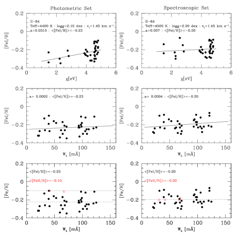
Figure 3: Demonstration of the offset in temperature, surface gravity, and metallicity found for the star II-64 based on photometric and spectroscopic methods. The constant $\tt a$ is the slope of the least-squares fit to the data. $\it Top$: FeI vs. $\chi$. $\it Middle$: FeI vs. W_λ. $\it Bottom$: FeI ($\it circles$) and FeII ($\it squares$) vs. W_λ. The dotted line corresponds to the mean values found using only those measured within 1 $\sigma$, as employed by the $\sigma$ clipping method.

3.3 Final parameters and metallicity

To derive metallicities, Fe I and Fe II lines with 15 $<$ W_λ $<$ 150 m$\rm\AA$ and $\lambda>$ 5800 $\rm\AA$ were selected. Photospheric 1D models for the sample giants were extracted from the NMARCS grid (Plez et al. 1992).

The LTE abundance analysis and the spectrum synthesis calculations were performed using the codes by Spite (1967) and subsequent improvements in the last thirty years, described in Cayrel et al. (1991) and Barbuy et al. (2003).

Stellar parameters were derived by initially adopting the photometric effective temperature and gravity and then further constraining the temperature by imposing excitation equilibrium for Fe I lines and the gravity by imposing ionization equilibrium for Fe I and Fe II, as described in previous sections. The entire process of defining the atmospheric parameters is iterated until a consistent set of model atmosphere parameters is finally obtained. Table  3 summarises the derived atmospheric parameters. We adopt the spectroscopic parameters for the subsequent analysis, having used the photometric parameters only as initial values; therefore, the uncertainties on the reddening described in Sect. 3.1 do not affect the final results. We point out otherwise that the good agreement between the spectroscopic and photometric parameters indicates that the reddening value adopted is satisfactory.

Table 3: Photometric and adopted spectroscopic stellar parameters

Star	Mbol	$T_{\rm eff}$	$v_{t}$	$\log g^{\rm a}$	[FeI/H]	[FeII/H]
	mag	K	km s-1	dex	dex	dex
Photometric
II-64 267122	+0.1987	4448	1.45	2.07	$-0.23$ $\pm$ 0.15	$-0.10$ $\pm$ 0.03
II-85 266938	$-1.6190$	3842	1.38	1.08	$-0.23$ $\pm$ 0.15	$-0.29$ $\pm$ 0.09
III-8 265717	+0.0653	4543	1.32	2.05	$-0.21$ $\pm$ 0.16	$-0.23$ $\pm$ 0.09
267092	+0.4672	4700	1.50	2.27	$-0.19$ $\pm$ 0.11	$-0.46$ $\pm$ 0.06
Spectroscopic
II-64 267122	—	4500	1.45	2.20	$-0.20$ $\pm$ 0.15	$-0.20$ $\pm$ 0.01
II-85 266938	—	3800	1.38	1.10	$-0.23$ $\pm$ 0.15	$-0.29$ $\pm$ 0.09
III-8 265717	—	4600	1.40	2.40	$-0.17$ $\pm$ 0.15	$-0.17$ $\pm$ 0.04
267092	—	4600	1.50	2.50	$-0.21$ $\pm$ 0.12	$-0.22$ $\pm$ 0.06

The mean offset in the $T_{\rm eff}$ values is 25 $\pm$ 48 K ($\sigma$ = 96, 4 stars) in the sense of spectroscopic minus photometric temperature. This means that the mean $T_{\rm eff}$ based on photometry is $\sim$25 K cooler than the spectroscopic ones. Along the iterative process of [Fe/H] determination, discrepant lines were clipped out within 1 $\sigma$ of the mean. Tests on the sample stars showed that a 2 $\sigma$ clipping gives differences of [Fe/H]$<\pm$0.01. A mean metallicity of [Fe/H] = $-0.20$ $\pm$ 0.01 ($\sigma$ = 0.02, 4 stars) is found for the sample stars. The spectroscopic parameters were adopted for the abundance analysis.

4 Spectrum synthesis

Abundance ratios were derived for the following eleven elements Na, Mg, Al, Si, Ca, Ti, Fe, Zr, Ba, La, and Eu. Most lines used are the same reported in Barbuy et al. (2006) as those Table A.1 gives the relevant parameters used in the spectrum synthesis of each line and resulting abundances.

Elemental abundances were obtained through line-by-line spectrum synthesis calculations with atomic lines as described in Sect. 3 and molecular lines of CN A²$\Pi$-X²$\Sigma$, C₂ Swan A³$\Pi$-X³$\Pi$ and TiO A³$\Phi$-X³$\Delta$ $\gamma$ and B³$\Pi$-X³$\Delta$ $\gamma$’ systems taken into account. Table 4 gives the final mean results for each star, where the abundances were normalized to FeI for neutral elements and FeII for ionized ones.

Abundances of the $\alpha$-elements Mg, Ca, Si, and Ti were derived. The oxygen forbidden line at 6300 ${\rm\AA}$ is blended with the strong sky emission line, given the low radial velocity of the cluster (Sect. 2.3), cannot be studied. In a previous work, Meléndez et al. (2003) derived the oxygen abundance of 5 giants in NGC 6553, based on OH infrared lines. We adopted the carbon, nitrogen, and oxygen abundances from that work in the present calculations, namely [C/Fe]=$-$0.7, [N/Fe]= +1.30, [O/Fe]=+0.25. Figures 4 and 5 show the magnesium triplet at 6318.7, 6319.2, 6319.4 ${\rm\AA}$, and SiI 5948.548 ${\rm\AA}$ in the giant II-85. Figure 6 shows the Europium line at 6645.127 ${\rm\AA}$ in II-85.

Table 4: Mean abundance ratios of the programme stars and final mean cluster abundances derived

		II-64			II-85			III-8			267092		mean
Species	$\epsilon_{\odot}$(X)a	N	[X/Fe]		N	[X/Fe]		N	[X/Fe]		N	[X/Fe]	[X/Fe]
$\alpha$-elements
Mg I	7.58	3	+0.32 $\pm$ 0.09		3	+0.27		3	+0.29 $\pm$ 0.03		3	+0.22 $\pm$ 0.09	+0.28 $\pm$ 0.04
Si I	7.55	6	+0.27 $\pm$ 0.09		4	+0.22 $\pm$ 0.08		6	+0.17 $\pm$ 0.07		6	+0.17 $\pm$ 0.03	+0.21 $\pm$ 0.05
Ca I	6.36	15	$+$0.11 $\pm$ 0.12		14	$+$0.12 $\pm$ 0.09		15	$+$0.05 $\pm$ 0.14		15	$-$0.07 $\pm$ 0.13	+0.05 $\pm$ 0.09
Ti I	5.02	15	$+$0.04 $\pm$ 0.08		15	+0.15 $\pm$ 0.11		15	$-$0.05 $\pm$ 0.10		15	$-$0.17 $\pm$ 0.15	$-$0.01 $\pm$ 0.14
Ti II	5.02	2	$+$0.06 $\pm$ 0.04		2	$+$0.01 $\pm$ 0.11		2	$-$0.04 $\pm$ 0.04		2	$-$0.07	$-$0.02 $\pm$ 0.06
Odd-Z elements
Na I	6.33	2	+0.12		3	+0.34		2	$-$0.08		2	+0.12	+0.16 $\pm$ 0.23
Al I	6.47	2	+0.25 $\pm$ 0.03		—	—		2	+0.15 $\pm$ 0.17		2	+0.13	+0.18 $\pm$ 0.06
Heavy elements
Zr I	2.60	1	$-0.74$		1	$-0.64$		1	$-0.64$		1	$-0.64$	$-$0.67 $\pm$ 0.05
Ba II	2.13	2	$-$0.08		2	$-$0.18 $\pm$ 0.14		2	$-$0.48 $\pm$ 0.14		2	$-$0.38	$-$0.28 $\pm$ 0.18
La II	1.17	1	+0.01		1	$-0.22$		—	—		—	—	$-$0.11 $\pm$ 0.16
Eu II	0.51	1	+0.09		1	+0.09		1	+0.10		1	+0.14	+0.10 $\pm$ 0.02
[Fe/H]
Fe I	7.50	56	$-0.20$ $\pm$ 0.15		52	$-0.23$ $\pm$ 0.15		59	$-0.17$ $\pm$ 0.15		57	$-0.21$ $\pm$ 0.12	$-$0.20 $\pm$ 0.02
Fe II	7.50	4	$-0.20$ $\pm$ 0.01		2	$-0.29$ $\pm$ 0.09		3	$-0.17$ $\pm$ 0.04		4	$-0.22$ $\pm$ 0.06	$-0.22$ $\pm$ 0.05

• Solar abundances are from Grevesse & Sauval (1998).

4.1 Errors in abundance ratios

Abundances for each species given in Table 4 were obtained by averaging the abundances resulting from all measured lines. Consequently, we give the 1 $\sigma$ scatter (standard deviation) of each measurement, such that the standard error can be obtained easily.

The uncertainties on atmospheric parameters were discussed in Sect. 3. To estimate the uncertainties on the derivation of abundances due to the choice of stellar parameters, we show the sensitivity of the abundances in Table 5 for the star II-64 by varying the temperature by 100 K, surface gravity by +0.30 dex, and microturbulent velocity by +0.20 km s^-1, which are typical errors in our analysis. The total error is given in the last column as the quadratic sum of all uncertainties. We can see that the total uncertainties are lower than 0.21 dex. In the next sections these uncertainties correspond to the 1 $\sigma$ scatter for each atomic species.

Table 5: Sensitivity of abundances to changes in $\Delta$T_eff = 100 K, $\Delta$log g = +0.3, and $\Delta$v_t = 0.2 km s^-1. In the last column the corresponding total error is given.

Species	$\Delta$T	$\Delta$$\log$ g	$\Delta$vt	($\sum$x2)1/2
(1)	(2)	(3)	(4)	(5)
II-64
[NaI/Fe]	+0.08	+0.02	$-$0.02	+0.08
[MgI/Fe]	$-$0.01	$-$0.02	+0.01	+0.02
[AlI/Fe]	+ 0.10	+0.00	+0.01	+0.10
[SiI/Fe]	$-$0.10	$-$0.01	$-$0.05	+0.11
[CaI/Fe]	+0.05	+0.01	$-$ 0.15	+0.16
[TiI/Fe]	+0.10	+0.03	$-$ 0.10	+0.14
[TiII/Fe]	+0.05	+0.20	+0.05	+0.21
[ZrI/Fe]	+0.20	+0.01	+0.01	+0.20
[BaII/Fe]	+0.01	+0.05	$-$ 0.20	+0.21
[LaII/Fe]	+0.01	+0.05	+0.02	+0.05
[EuII/Fe]	+0.01	+0.06	+0.01	+0.06
[FeI/H]	$-$0.03	$-$0.04	+0.07	+0.09
[FeII/H]	+0.12	$-$0.11	+0.06	+0.17

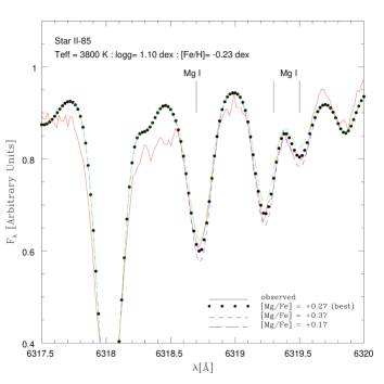
Figure 4: Magnesium triplet at 6318.7, 6319.2, 6319.4 ${\rm\AA}$ in II-85 computed with [Mg/Fe] = +0.27 (dotted line, best fit), [Mg/Fe] = +0.37 (short-dashed line), and [Mg/Fe] = +0.17 (long-dashed line).

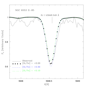
Figure 5: Silicon line at 5948.548 ${\rm\AA}$ in II-85 computed with [Si/Fe] = +0.20 (dotted line, best fit), [Si/Fe] = +0.30 (short-dashed line), and [Si/Fe] = +0.10 (long-dashed line).

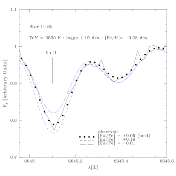
Figure 6: Europium line at 6645 ${\rm\AA}$ in II-85 computed with [Eu/Fe] = +0.09 (dotted line, best fit), [Eu/Fe] = +0.19 (short-dashed line), and [Eu/Fe] = $-$0.01 (long-dashed line).

4.2 Comparison with previous work

In the present work a metallicity of [Fe/H]=$-$0.20 is found for NGC 6553. A derivation based on photometric parameters gives [FeI/H]=$-$0.22 and [FeII/H]=$-$0.21, whereas for star 267092 it gives [FeI/H]=$-$0.19 and [FeII/H]=$-$0.46. In other words, the metallicities are the same whether they are computed with the photometric or the spectroscopic parameters, since the two sets of parameters are similar; and as demonstrated in Fig. 3, the spectroscopic parameters give a better agreement between the four stars than the photometric ones.

4.2.1 Comparison with Barbuy et al. (1992)

In Barbuy et al. (1992) a metallicity of [Fe/H]=$-$0.20 was found, in agreement with the present work. A reddening E(B-V)=0.73 and a photometric effective temperature was adopted. Despite the much lower S/N of those spectra, the overall fit of synthetic spectra, which take blanketing lowering the continuum into account, proved to be a satisfactory method.

4.2.2 Comparison with Barbuy et al. (1999)

The atmospheric parameters adopted for II-85, the single star in common with the present work, were T_eff=4000 K, log g = 1.26 (0.70), v_t=1.30 km s^-1 and [Fe/H]=$-$0.50. The VI colours obtained with HST (Ortolani et al. 1995) were used, which differ slightly from the WFI ones used in the present paper.

We found 3 main sources of uncertainty in the metallicity of [Fe/H]=$-$0.55 found in Barbuy et al. (1999), by comparing the parameters of star II-85 in common with the present work.

(i) The effective temperature of 4000 K was derived in Barbuy et al. (1999) using photometry, adopting a reddening of E(B-V)=0.70, whereas in the present work a spectroscopic excitation temperature of 3842 K is obtained.

(ii) The main source of discrepancy has been an inappropriate correction of gravity by 0.60 dex. The difference of log g = 1.26 found then from classical formulae and log g = 0.70 as adopted led to a $\Delta$[Fe/H]=$-$0.3.

(iii) Equivalent widths for the star II-85 for lines in common are compared in Table 6. It appears that in the early work of 1999, W_λ’s of strong lines were systematically lower by about 20 m${\rm\AA}$, which leads to a metallicity that is lower by $\Delta$[Fe/H] $\approx$ 0.1 dex. The reason for the discrepancy in W_λ’s comes from the lower quality of the 1999 CASPEC spectra both in resolution and S/N. This can be seen in Fig. 7, which compares the two sets of observations for the star II-85.

Table 6: FeI lines used in the present work in common with Barbuy et al. (1999).

${\lambda({\rm\AA})}$	${\chi_{\rm ex}}$(eV)	log gf	Present	Barbuy et al. 1999
5861.110	4.280	-2.450	24.9	25.
6082.710	2.220	-3.570	131.1	102.
6096.660	3.980	-1.930	70.1	74.
6120.250	0.910	-5.950	96.4	69.
6475.620	2.560	-2.940	127.5	118.
6481.870	2.280	-2.980	148.5	117.
6574.230	0.990	-5.040	149.3	130.
6739.520	1.560	-4.940	98.4	49.

4.2.3 Comparison with Cohen et al. (1999)

The five stars of Cohen et al. were red horizontal branch stars with T_eff=4630-4830 K, log g=2.3, v_t=1.4-2.5 km s^-1, and a mean metallicity of [FeI/H]=-0.16 and [FeII/H]=$-$0.18. Effective temperatures were adopted from excitation equilibrium of FeI lines. In order to be compatible with the colours, they deduced E(B-V)=0.78 for 3 stars and E(B-V)=0.86 for the other two stars. The metallicity is in good agreement with the present work, whereas there is some discrepancy concerning the abundance ratios, as shown in Table 7. A difference $\Delta$[Ca/Fe]=0.2 is explained by an offset in the solar Ca abundance adopted (Table 7), whereas the oscillator strengths for the lines in common agree. No lines in common are available for comparing Ti oscillator strengths, but there is an offset in the solar abundance of $\Delta$[Ti/Fe]=0.05. Possible differences in damping constants cannot be checked since they are not given in Cohen et al. (1999).

Table 7: Comparison of solar abundances and abundance ratios obtained for NGC 6553 between the present work and Cohen et al. (1999).

	Present work		Cohen et al. 1999
Element	$\epsilon$⊙(X)	[X/Fe]	$\epsilon$⊙(X)	[X/Fe]
O	8.77	+0.2	8.68	+0.50
Mg	7.58	+0.28	7.54	+0.41
Si	7.55	+0.21	7.54	+0.14
Ca	6.36	+0.05	6.16	+0.26
Ti	5.02	-0.01	4.98	+0.19

4.2.4 Comparison with Origlia et al. (2002)

Origlia et al. (2002) analysed 2 stars of T_eff=4000 K, log g=1.0, v_t=2 km s^-1, and a mean metallicity of [FeI/H]=$-$0.30 was derived, together with enhancement of oxygen [O/Fe]=+0.30, and [$\alpha$/Fe]=+0.30 (Mg, Ca and Si). A reddening of E(J-K)=0.41, compatible with E(B-V)=0.70, was used.

4.2.5 Comparison with Meléndez et al. (2003)

The parameters of II-85, again in common with the present work, of T_eff=4000 K, log g=1.2, v_t=1.4 km s^-1, [Fe/H]=$-$0.20, found in Meléndez et al. (2003), show an effective temperature higher by 200 K, in agreement with Barbuy et al. (1999). As in Barbuy et al. (1999), the VI colours from HST (Ortolani et al. 1995) were used, as well as a reddening of E(B-V)=0.70. Despite the difference with the present work, the resulting metallicities agree, which is explained by the low sensitivity of the high excitation potential infrared FeI lines to T_eff (see Table 6 in Meléndez et al. 2003).

Figure 7: Spectra of the giant II-85: comparison between the spectrum studied in Barbuy et al. (1999), obtained with the 3.6m telescope and the CASPEC spectrograph (R $\sim$ 20 000) and the present spectrum obtained with VLT-UVES (R$\sim$55 000).

5 Abundance ratios

5.1 $\alpha$-elements Mg, Ca, Si, Ti

The $\alpha$-elements provide information on the relative contributions of SNe type II and Ia in the enrichment of the interstellar medium prior to the formation of cluster stars. Type II Supernovae are the main sources of $\alpha$-elements (Woosley & Weaver 1995), the yields depending upon the mass of the progenitor.

Magnesium and silicon are moderately enhanced with [Mg/Fe] = +0.28 $\pm$ 0.04 and [Si/Fe] = +0.21 $\pm$ 0.05 dex. A solar calcium-to-iron [Ca/Fe] = +0.05 $\pm$ 0.09 dex and titanium-to-iron [TiI/Fe] = $-$0.01 $\pm$ 0.14 and [TiII/Fe] = $-$0.02 $\pm$ 0.06 are found. In Fig. 8 $\alpha$-element abundances from the present work (Table 4), Meléndez et al. (2003), and Cohen et al. (1999) are shown as a function of Atomic Number Z. While in Cohen et al. (1999), O, Mg, Si, Ca, and Ti are enhanced, in the present work Ca and Ti are solar, whereas Si and Mg are enhanced. The high oxygen abundance in Cohen et al. (1999), relative to the value found by Meléndez et al. (2003), may be due to the use of the OI 771-7 nm triplet that systematically gives higher abundances (Kiselman 1995). Besides, there is an offset in the solar oxygen abundance adopted (Table 6) of $\Delta$[O/Fe]=0.09. The mean abundance of [Ti/Fe] in NGC 6553 resembles the value found in Zoccali et al. (2004) for NGC 6528, obtained using the same atomic parameters.

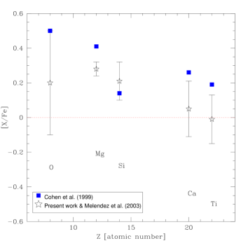
Figure 8: Abundance pattern in $\alpha$-elements in NGC 6553 corresponding to: (i) a mean of the four sample stars derived in the present work and adopting oxygen from Meléndez et al. (2003) (open stars) and (ii) abundances of the same elements given in Table 5 of Cohen et al. (1999) (filled squares).

5.2 Odd-Z elements Na, Al

Sodium and aluminum are odd-Z elements produced by neutron capture in the Ne-Na and Mg-Al cycles during carbon burning. A mean value of [Na/Fe] = +0.16 $\pm$ 0.23 dex and [Al/Fe] = +0.18 $\pm$ 0.06 dex are found. No corrections for non-LTE effects were applied. The red giant II-85 of our sample is enhanced in Na by [Na/Fe]=+0.34 dex, while the other stars show solar ratios. This result is compatible with a mixing occurring along the RGB (Gratton et al. 2004), and to check this, it would be interesting to derive nitrogen abundances for our sample stars. Na is compatible with results by McWilliam & Rich 1994, hereafter MR94); on the other hand, it is overabundant in NGC 6528 (Zoccali et al. 2004). A moderate enhancement of Aluminum of [Al/Fe]=+0.18 is found.

5.3 Heavy elements Zr, Ba, La, Eu

The s-process elements Zr, Ba, and La are produced through neutron-capture in asymptotic giant branch stars (Käppeler 1989; Busso et al. 1999). Abundances of the s- (Zr, Ba, and La) elements obtained were [Zr/Fe] = $-$0.67 $\pm$ 0.05, [Ba/Fe] = $-$0.28 $\pm$ 0.18, and [La/Fe] = $-$0.11 $\pm$ 0.16. Barium is depleted by $-$0.28 dex in NGC 6553, in contrast to an enhanced Ba abundance in 47 Tuc (Alves-Brito et al. 2005), a moderate enhancement in MR94, and a solar value in NGC 6528 (Zoccali et al. 2004). All s-elements are depleted. Edvardsson et al. (1993) show that [Ba/H] is a better age indicator than [Fe/H]. Low s-element abundances suggest that the cluster is old, confirming the findings from CMDs (Ortolani et al. 1995).

The r-element europium abundance is [Eu/Fe] = +0.10 $\pm$ 0.02 dex. This moderate overabundance of Eu-to-Fe is compatible with those of the $\alpha$-elements, these elements being all produced by SNe II.

6 Conclusions

A detailed analysis based on high-resolution spectra for four giants of the metal-rich bulge globular cluster NGC 6553 was carried out. The present spectra are the highest resolution data so far for stars in this cluster. We find a mean metallicity value of [Fe/H]=$-$0.20, in agreement with Cohen et al. (1999) and Meléndez et al. (2003).

The $\alpha$-elements Mg and Si are overabundant relative to Fe with [Mg/Fe] = +0.28 dex and [Si/Fe] = +0.21 dex, which might indicate a rapid chemical evolution history dominated by Type II Supernovae in the Galactic bulge. The lower abundances for the $\alpha-$elements Ca ([Ca/Fe] = +0.05 dex) and Ti ([Ti/Fe] = $-$0.01 dex) in stars of NGC 6553 might suggest a deficiency of low-mass Type II supernovae. The s-process elements Zr, Ba, and La are depleted by [Zr/Fe]=$-$0.67 dex, [Ba/Fe]=$-$0.28, and [La/Fe]=$-0.11$ dex, respectively. The underabundance of s-elements is an independent indication that the cluster is old (Edvardsson et al. 1993). The r-process element Eu shows a small enhancement of [Eu/Fe] =+0.10 dex, as do the $\alpha-$elements Ca and Ti. NGC 6553 appears to be very similar in its element abundance ratios to NGC 6528 analysed in Zoccali et al. (2004). The two clusters are very similar in age and metallicity, as pointed out in Ortolani et al. (1995).

Whether the metal-rich bulge clusters were formed during an early collapse or in merging events, as expected in hierarchical scenarios, can be revealed by abundance ratios. An early formation is accompanied by $\alpha$-enhancement. However in merging events, no detailed models are available: it is even possible that merging truncates star formation (Di Matteo et al. 2005). If instead bulge formation occurred via secular evolution of a bar (Kormendy & Kennicutt 2004), solar abundance ratios would be expected, but this is not the case for NGC 6553. At the present time, it is important to gather metallicities and abundance ratios for other metal-rich clusters in the Galactic bulge, since their age spread and chemical abundances can constrain different models of bulge formation (Bekki 2005; Beasley et al. 2002; van den Bergh 1993).

Appendix A Line list

[x]lccccccccr

Line list used for synthesis showing species, wavelength, excitation potential, damping constant, gf-values, and abundances derived line-by-line.

[X/Fe]

Species $\lambda$(Å) $\chi_{ex}$(eV) $C6$ log $gf$ II-64 II-85 III-8 267092

continued.
[X/Fe]

Species $\lambda$(Å) $\chi_{ex}$(eV) $C6$ log $gf$ II-64 II-85 III-8 267092

$\alpha$-elements
Mg I 6318.720 5.110 0.30E$-$31 $-2.100$ +0.27 +0.27 +0.27 +0.12
Mg I 6319.242 5.110 0.30E$-$31 $-2.360$ +0.27 +0.27 +0.27 +0.27
Mg I 6319.490 5.110 0.30E$-$31 $-2.900$ +0.42 +0.27 +0.35 +0.27

Si I 5948.548 5.082 2.19E-30 $-1.170$ +0.20 +0.20 +0.25 +0.15
Si I 6142.490 5.620 0.30E$-$31 $-1.580$ +0.20 +0.12 +0.10 +0.20
Si I 6145.020 5.610 0.30E$-$31 $-1.500$ … +0.25 … …
Si I 6155.020 5.620 0.30E$-$30 $-0.850$ +0.40 +0.30 +0.25 +0.20
Si I 6243.823 5.610 0.30E$-$32 $-1.300$ +0.35 … +0.10 +0.15
Si I 6244.480 5.610 0.30E$-$31 $-1.270$ +0.30 … +0.15 +0.15
Si I 6414.987 5.870 0.30E$-$30 $-1.128$ +0.20 … +0.15 +0.15

Ca I 6102.723 1.879 4.54E$-$31 $-0.930$ +0.09 +0.14 +0.09 $-$0.11
Ca I 6156.030 2.521 4.00E$-$31 $-2.590$ +0.14 +0.09 +0.09 $-$0.01
Ca I 6161.297 2.523 4.00E$-$31 $-1.420$ +0.14 +0.24 +0.14 $-$0.01
Ca I 6162.173 2.523 3.00E$-$31 $-0.090$ +0.09 +0.09 +0.14 $-$0.01
Ca I 6166.439 2.521 3.97E$-$31 $-1.156$ +0.09 +0.09 $-$0.01$-$0.06
Ca I 6169.042 2.523 3.97E$-$31 $-0.900$ +0.29 +0.19 +0.14 $-$0.06
Ca I 6169.563 2.526 4.00E$-$31 $-0.630$ +0.29 +0.19 +0.14 $-$0.11
Ca I 6439.075 2.526 3.40E$-$32 $+0.300$ +0.14 +0.09 +0.14 $-$0.11
Ca I 6455.598 2.523 3.39E$-$32 $-1.550$ +0.19 +0.09 +0.14 +0.04
Ca I 6464.679 2.520 3.40E$-$32 $-2.480$ +0.24 $-$0.06 +0.24 +0.24
Ca I 6471.662 2.526 3.39E$-$32 $-0.800$ +0.09 +0.19 +0.09 $-$0.21
Ca I 6493.788 2.526 3.37E$-$32 $+0.000$ $-$0.11 +0.19 $-$0.21$-$0.21
Ca I 6499.654 2.526 3.37E$-$32 $-0.850$ $-$0.11 +0.19 $-$0.21$-$0.06
Ca I 6508.850 2.526 3.37E$-$32 $-2.510$ +0.09 $-$0.06$-$0.06$-$0.11
Ca I 6572.778 0.000 1.75E$-$32 $-4.320$ $-$0.01… $-$0.16$-$0.31

Ti I 5866.452 1.067 2.16E$-$32 $-0.840$ +0.18 +0.28 +0.13 +0.03
Ti I 5965.828 1.879 2.14E$-$32 $-0.409$ +0.13 +0.06 +0.13 $-$0.12
Ti I 5978.543 1.873 2.14E$-$32 $-0.496$ +0.18 +0.06 +0.08 $-$0.12
Ti I 6064.629 1.046 2.06E$-$32 $-1.944$ +0.03 +0.31 $-$0.17 $-$0.17
Ti I 6091.174 2.267 3.89E$-$32 $-0.423$ +0.03 +0.26 +0.03 $-$0.12
Ti I 6126.217 1.067 2.06E$-$32 $-1.424$ +0.03 +0.31 +0.03 $-$0.47
Ti I 6258.110 1.440 4.75E$-$32 $-0.360$ $-$0.07 +0.11 $-$0.17 $-$0.52
Ti I 6303.756 1.443 1.53E$-$32 $-1.566$ +0.08 +0.06 $-$0.07 $-$0.12
Ti I 6312.237 1.460 4.75E$-$32 $-1.552$ +0.08 +0.11 $-$0.07 $-$0.07
Ti I 6336.102 1.443 0.30E$-$31 $-1.742$ $-$0.02 +0.11 $-$0.07 $-$0.07
Ti I 6508.153 1.430 1.46E$-$32 $-2.050$ +0.03 +0.11 $-$0.07 $-$0.07
Ti I 6554.224 1.443 2.72E$-$32 $-1.219$ +0.03 +0.11 $-$0.17 $-$0.17
Ti I 6556.062 1.460 2.74E$-$32 $-1.075$ +0.03 $-$0.04$-$0.17 $-$0.22
Ti I 6599.130 0.900 2.94E$-$32 $-2.085$ $-$0.02 +0.26 $-$0.07 $-$0.27
Ti I 6743.124 0.900 0.30E$-$31 $-1.628$ $-$0.07 +0.26 $-$0.07 $-$0.07
Ti II 6491.582 2.060 0.30E$-$31 $-2.100$ +0.03 +0.08 $-$0.07 $-$0.07
Ti II 6559.576 2.050 0.30E$-$31 $-2.480$ +0.09 $-$0.07$-$0.02 $-$0.07

Odd-Z elements

Na I 5682.647 2.102 0.30E$-$30 $-$0.700 … +0.34 … …
Na I 5688.217 2.102 0.30E$-$30 $-$0.457 … +0.34 … …
Na I 6154.225 2.102 0.90E$-$31 $-1.570$ +0.12+0.34$-$0.08 +0.12
Na I 6160.753 2.104 0.30E$-$31 $-1.270$ +0.12 … $-$0.08 +0.12
Al I 6696.032 3.143 0.30E$-$31 $-1.481$ +0.28 … +0.28 +0.13
Al I 6698.667 3.143 0.30E$-$31 $-1.782$ +0.23 … +0.03 +0.13

Heavy elements
Zr I 6143.216 0.070 0.30E$-$31 $-1.100$ $-0.74$ $-0.64$ $-0.64$ $-0.64$
Ba II 6141.728 0.704 $-0.070$ $-0.08$ $-0.28$ $-0.58$ $-0.38$
Ba II 6496.900 0.604 $-0.380$ $-0.08$ $-0.08$ $-0.38$ $-0.38$
La II 6390.483 0.320 $-1.410$ +0.01 $-0.22$ … …
Eu II 6645.127 1.380 $+0.120$ +0.09 +0.09 +0.10 +0.14

[x]lcccccccc

Fe I and Fe II line list: (1) element, (2) wavelength, (3) lower excitation potential, (4) log $gf$-values, (5)-(8) equivalent widths [m$\rm\AA$].

Ion $\lambda$[Å] $\chi_{ex}$ [eV] log $gf$ II-64 II-85 III-8 267092
(1) (2) (3) (4) (5) (6) (7) (8)

continued.

Ion $\lambda$[Å] $\chi_{ex}$ [eV] log $gf$ II-64 II-85 III-8 267092
(1) (2) (3) (4) (5) (6) (7) (8)

Fe I

Fe I 5833.93 2.61 $-3.66$ … … 55.2 …
Fe I 5835.10 4.26 $-2.37$ 39.8 30.0 … …
Fe I 5853.15 1.48 $-5.27$ 59.7 88.3 44.8 48.0
Fe I 5855.08 4.60 $-1.75$ 39.6 47.6 41.6 38.7
Fe I 5856.09 4.29 $-1.64$ 61.7 66.7 57.3 62.0
Fe I 5858.78 4.22 $-2.26$ 29.3 36.6 28.8 28.9
Fe I 5859.60 4.55 $-0.60$ 94.7 88.5 91.9 91.1
Fe I 5861.11 4.28 $-2.45$ 20.6 24.9 16.9 26.5
Fe I 5862.37 4.55 $-0.39$ 108.1 95.9 102.6 107.1
Fe I 5881.28 4.60 $-1.84$ … 34.8 38.0 35.1
Fe I 5902.47 4.59 $-1.81$ 24.1 24.5 26.2 23.8
Fe I 5905.67 4.65 $-0.72$ 74.7 67.4 78.3 74.4
Fe I 5927.79 4.65 $-1.09$ 64.7 65.1 67.8 65.6
Fe I 5929.68 4.55 $-1.39$ 75.2 63.8 75.6 61.5
Fe I 5930.18 4.65 $-0.23$ 121.3 102.6 118.7 120.0
Fe I 5934.65 3.93 $-1.18$ 111.3 106.0 106.9 108.6
Fe I 5952.72 3.98 $-1.43$ 97.2 82.0 91.0 94.7
Fe I 5956.69 0.86 $-4.60$ 137.6 … 126.1 120.6
Fe I 5969.56 4.28 $-2.73$ … 15.8 … …
Fe I 5983.69 4.55 $-0.78$ 97.5 83.4 81.8 91.6
Fe I 5987.07 4.79 $-0.45$ 93.2 84.7 92.0 95.9
Fe I 6003.01 3.88 $-1.11$ 119.7 106.9 119.2 113.9
Fe I 6024.06 4.55 $-0.11$ 124.8 107.7 121.0 119.1
Fe I 6027.05 4.07 $-1.22$ 98.4 87.5 79.1 95.5
Fe I 6054.07 4.37 $-2.30$ 22.2 30.3 27.1 23.6
Fe I 6056.01 4.73 $-0.46$ 85.5 83.4 112.0 90.8
Fe I 6078.50 4.79 $-0.40$ 99.0 86.9 96.2 95.4
Fe I 6079.01 4.65 $-1.13$ 67.8 64.5 66.3 68.6
Fe I 6082.71 2.22 $-3.57$ 100.9 131.1 87.5 90.0
Fe I 6093.64 4.60 $-1.51$ 53.0 49.8 53.0 48.8
Fe I 6094.37 4.65 $-1.94$ 37.4 35.9 35.2 34.1
Fe I 6096.66 3.98 $-1.93$ 68.5 70.1 67.2 66.1
Fe I 6098.28 4.56 $-1.88$ 33.0 46.5 39.1 37.0
Fe I 6105.13 4.54 $-2.06$ 31.8 43.0 30.2 28.0
Fe I 6120.25 0.91 $-5.95$ 59.7 96.4 52.4 45.0
Fe I 6353.85 0.91 $-6.36$ … 71.7 … …
Fe I 6392.54 2.28 $-4.03$ 71.7 … 56.9 57.0
Fe I 6419.95 4.73 $-0.25$ 107.5 97.8 101.5 105.1
Fe I 6475.62 2.56 $-2.94$ 121.3 127.5 110.5 103.3
Fe I 6481.87 2.28 $-2.98$ 141.2 148.5 121.1 123.1
Fe I 6498.94 0.96 $-4.70$ 140.4 … 124.6 126.6
Fe I 6518.37 2.83 $-2.75$ 105.0 120.1 102.8 105.8
Fe I 6533.93 4.56 $-1.45$ 69.5 58.5 61.3 66.8
Fe I 6556.81 4.79 $-1.68$ 24.3 28.4 30.0 25.6
Fe I 6569.22 4.73 $-0.42$ 105.5 102.0 100.2 101.6
Fe I 6574.23 0.99 $-5.04$ 114.3 149.3 102.3 98.5
Fe I 6575.02 2.59 $-2.82$ … … 119.3 120.3
Fe I 6591.31 4.59 $-2.06$ 23.4 … 21.6 25.6
Fe I 6593.87 2.43 $-2.42$ … … 142.2 148.5
Fe I 6597.56 4.80 $-1.06$ 64.4 60.3 62.1 69.6
Fe I 6608.03 2.28 $-4.04$ 70.5 … 59.7 56.6
Fe I 6699.14 4.59 $-2.18$ 29.4 25.8 24.7 20.7
Fe I 6703.57 2.76 $-3.15$ 93.4 96.5 82.6 84.5
Fe I 6705.11 4.61 $-1.40$ 77.2 58.5 72.7 74.2
Fe I 6710.32 1.48 $-4.87$ 94.6 112.1 83.1 79.3
Fe I 6713.74 4.80 $-1.60$ 40.0 33.1 36.7 37.9
Fe I 6715.38 4.59 $-1.64$ 65.3 … 57.6 …
Fe I 6725.36 4.10 $-2.30$ 41.1 41.5 39.2 41.5
Fe I 6726.67 4.59 $-1.15$ 71.5 56.4 67.6 66.7
Fe I 6733.15 4.64 $-1.58$ 48.7 54.6 52.8 50.4
Fe I 6739.52 1.56 $-4.94$ 72.2 98.4 64.0 57.2
Fe I 6752.71 4.64 $-1.37$ 74.7 … 66.4 62.8
Fe II

Fe II 5991.36 3.15 -3.54 … … 43.4 …
Fe II 6084.09 3.20 -3.79 31.2 … 31.7 …
Fe II 6149.24 3.89 -2.69 … … 51.4 …
Fe II 6247.56 3.89 -2.30 … … 50.7 54.7
Fe II 6432.68 2.89 -3.57 42.0 29.1 53.8 55.9
Fe II 6456.39 3.90 -2.05 69.3 33.5 72.2 64.5
Fe II 6516.08 2.89 -3.31 66.9 … … 69.3