The effect of inhomogeneous expansion on the supernova observations

Abstract:

We consider an inhomogeneous but spherically symmetric Lemaitre-Tolman-Bondi model to demonstrate that spatial variations of the expansion rate can have a significant effect on the cosmological supernova observations. A model with no dark energy but a local Hubble parameter about $15$ % larger than its global value fits the supernova data better than the homogeneous model with the cosmological constant. The goodness of the fit is not sensitive to inhomogeneities in the present-day matter density, and our best fit model has $\Omega_{M}(r)\sim 0.3$, in agreement with galaxy surveys. We also compute the averaged expansion rate, defined by the Buchert equations, of the best fit model and show explicitly that there is no average acceleration.

1 Introduction

The simplest homogeneous and isotropic cosmological model within the framework of general relativity is parameterized by two numbers: the Hubble constant $H_{0}$ and the density parameter $\Omega_{M}$, interpreted respectively as the average expansion rate and the average density of non-relativistic matter in the present universe. This model was generally considered a good description of the universe on the largest scales until the high redshift supernova observations in the late 90’s [1]. With the latest data from supernovae [2, 3], galaxy distributions [4] and anisotropies of the cosmic microwave background [5] the simplest homogenous and isotropic model would now lead to a highly contradictory picture of the universe, as the best fit values of this model for the average matter density demonstrate:

• Cosmic microwave background: $\Omega_{M}\sim 1$

• Galaxy surveys: $\Omega_{M}\sim 0.3$

• Type Ia supernovae: $\Omega_{M}\sim 0$

The natural conclusion is that at least one of the assumptions of the model must be false.

As is well known, the problem has conventionally been remedied by introducing the cosmological constant $\Lambda$ or vacuum energy $\Omega_{\Lambda}$, giving rise to an accelerated expansion of the universe. Indeed, the analysis of the cosmological data with both the vacuum energy and matter components included yields a consistent picture of the universe, known as the concordance $\Lambda$CDM model, with the following best fit values for the density parameters:

• Cosmic microwave background: $\Omega_{M}+\Omega_{\Lambda}\sim 1$

• Galaxy surveys: $\Omega_{M}\sim 0.3$

• Type Ia supernovae: $\Omega_{M}\sim 0.3$ and $\Omega_{\Lambda}\sim 0.7$

Moreover, the data seems to require $\Omega_{\Lambda}>0$ at a high confidence level [2, 3].

Although the cosmological concordance $\Lambda$CDM model fits all the observations well, it is plagued by theoretical problems [6]. We do not have a theory that would explain, not to mention predict, the required value of the cosmological constant. Various dark energy models, which have been studied intensively in order to provide a dynamical explanation for the cosmological constant, are not compelling from the particle physics point of view and often require fine-tuning [6, 7]. Modifications of the general theory of relativity on cosmological scales appear to suffer from analogous problems; in fact, it has recently been argued that the cosmological constant seems to be essentially the only modification that fits all the cosmological data [8].

As a rejection of either matter domination or Einstein gravity leads to trouble, it is well motivated to study the validity of the third main assumption, the perfect homogeneity. Undoubtedly, at least on small scales, large inhomogeneities exist. Although the potential cosmological consequences of the inhomogeneities were recognized already around the same time when the homogeneous and isotropic models of the universe were first studied, their impact on the global dynamics of the universe is still unknown (see e.g. [9]). Indeed, the role of the inhomogeneities has often been debated whenever there have been some ambiguities with cosmological observations, for example, in the 90’s when in the determination of the age of the universe there was a discrepancy between the implications of cosmological and astronomical observations [10, 11].

Most recently, inhomogeneities have been invoked as the culprit for the apparent acceleration of the expansion of the universe, in particular by virtue of their so-called backreaction on the metric (for a recent discussion on the issues involved and a comprehensive list of references, see [13]). The problems in these approaches have been mainly of technical nature, as reducing the symmetries of the metric rapidly complicates the calculations. A lesser difficulty arises from the fact that different inhomogeneities can lead to identical observations [14], so that not even ideal observations of light could determine the inhomogeneities uniquely. As a consequence, there have been two conceptually distinct ways to approach the inhomogeneities: the first one examines the effect of the inhomogeneities on the expansion of the universe, whereas the second tries to determine their impact on the observations directly.

In the first approach an effective description of the universe is constructed by averaging out the spatial degrees of freedom, i.e. the inhomogeneities [13, 15, 16, 17]. As a result, one obtains averaged, effective Einstein equations which, in addition to terms found in the usual homogeneous case, include new terms that represent the effect of the inhomogeneities, called backreaction in this context. It has been argued that the backreaction might account for the accelerated expansion [13, 16, 18].

However, since we can only observe the redshift and energy flux of light arriving from a given source, not the expansion rate and the matter density of the universe nor their averages, one may wonder how the actual observables are related to the averaged equations. To wit, since we do not observe the expansion of the universe directly, its acceleration is also an indirect conclusion, arising from the fact that in the perfectly homogeneous cosmological models dark energy is required for a good fit. Consequently, there is no a priori reason to assume that the acceleration would be needed in the more general inhomogeneous models of the universe. Moreover, it is well recognized that in general it is not correct to integrate out constrained degrees of freedom as if they were independent. Indeed, the fact that we can make cosmological observations only along our past light cone makes the observable universe a constrained system.

The second approach avoids these problems by studying the effect of the inhomogeneities directly on the observable light [14, 19]. This would be virtually impossible in the presence of generic inhomogeneities but can be done in some simpler models, such as the spherically symmetric Lemaitre-Tolman-Bondi (LTB) model [20, 21, 22]. This model works best in describing smooth inhomogeneities at scales of $100$ ${\rm{Mpc}}$ and larger; the spherical symmetry prevents to use it as a model for the random small scale lumpiness caused by galaxies, as noted in [23]. Indeed, the LTB model has been used to study the effect of the smooth inhomogeneities on the cosmological observations by several authors [23, 24, 25, 26, 27, 28, 29, 30, 31, 32]; a common conception is that these models inevitably contradict the observed homogeneity of the large scale galaxy distribution.

Although spherical symmetry is probably an unrealistic assumption for the entire universe, the LTB model can be regarded as describing observations that have been averaged over the celestial sphere and it is therefore useful at least on two counts. First, it serves as a simple testing ground for the effect of the inhomogeneities on the cosmological observations. Second, as the fits can be performed unambiguously, it can be used to study the connection of the backreaction driven effective acceleration to the observations; both of these points will be examined in this work.

As mentioned in the beginning, two independent parameters ($H_{0}$ and $\Omega_{M}$) are needed to uniquely define the homogeneous matter dominated universe. In the presence of inhomogeneities, the values of these two quantities are needed at every spatial point; that is, the inhomogeneous dust models are defined by two functions of the spatial coordinates: $H_{0}(x^{i})$ and $\Omega_{M}(x^{i})$. As a consequence, there are inhomogeneities of two physically different kind: inhomogeneities in the matter distribution, and inhomogeneities in the expansion rate. Although their dynamics are coupled via the Einstein equation, as boundary conditions they are independent. This opens up the possibility for a universe with inhomogeneous expansion but homogeneous present-day matter distribution; a model of this kind could potentially fit the supernova data as well as the galaxy surveys without invoking dark energy.

The paper is organized as follows. Sect. 2 discusses the general properties of the spherically symmetric, inhomogeneous LTB model. In Sect. 3 we fit the LTB model with inhomogeneous expansion but homogeneous present-day matter distribution to the supernova observations. For completeness, we consider both the cases of pure dust and dust plus the cosmological constant. The initial conditions of these models are discussed in Sects. 3.7 and 3.8. In Sect. 4 we evaluate the expansion rate and shear in the appropriate averaged (the so-called Buchert [16]) equations and demonstrate that an accelerated average expansion is not needed to fit the supernova data. Finally, Sect. 5 contains our conclusions.

2 Spherically symmetric inhomogeneous LTB model

Since Einstein’s equations form a set of six independent non-linear second-order partial differential equations, it is impossible to treat the universe exactly with completely generic inhomogeneities. On the other hand, the perfectly homogeneous FRW model does not fit the observations without a fine-tuned cosmological constant or some other modification. Therefore, we make the next simplest approximation and use the spherically symmetric but inhomogeneous LTB model. The aim is to extract the leading order effects of the inhomogeneities on the supernova observations as well as to demonstrate the pitfalls one may encounter when using averaged Einstein equations.

The LTB model has been used for the supernova data fitting several times before [24, 26, 27, 28, 29, 23, 30]. However, there is a crucial physical difference between these models and ours. Namely, the earlier works have had inhomogeneities in the present-day matter distribution whereas we will focus on models with inhomogeneities only in the expansion rate. Moreover, to ease the comparison between the FRW model, familiar to all cosmologists, and the less-known LTB model, we will rewrite the equations in a form where the connection of the physically equivalent quantities between these two models becomes very transparent. To introduce the new notation, we will rederive the main results of the LTB model in Sects. 2.1 and 2.2.

2.1 The Lemaitre-Tolman-Bondi metric

Let us consider a spherically symmetric dust universe with radial inhomogeneities as seen from our location at the center. Choosing spatial coordinates to comove ($dx^{i}/dt=0$) with the matter, the spatial origin ($x^{i}=0$) as the symmetry center, and the time coordinate ($x^{0}\equiv t$) to measure the proper time of the comoving fluid, the line element takes the form

$$ds^{2}=-dt^{2}+\frac{(A^{\prime}(r,t))^{2}}{1-k(r)}dr^{2}+A^{2}(r,t)\left(d\theta^{2}+\sin^{2}\theta d\varphi^{2}\right)~{},$$ (1)

where $k(r)$ is a function associated with the curvature of $t={\rm{const.}}$ hypersurfaces, the scale function $A(r,t)$ has both temporal and spatial dependence, and we use the following shorthand notations for the partial derivatives: ${}^{\prime}\equiv\frac{\partial}{\partial r}$ and $\dot{}\equiv\frac{\partial}{\partial t}$. This metric was first studied by Lemaitre [20], Tolman [21] and Bondi [22]; later, it has been used in various astronomical and cosmological contexts [9]. Note that the homogeneous and isotropic FRW metric is a special case of Eq. (1), obtained in the limit: $A(r,t)\rightarrow a(t)r$ and $k(r)\rightarrow kr^{2}$, where $a(t)$ is the FRW scale factor and $k$ is the curvature constant.

The energy momentum tensor in the above defined coordinates is given by

$$T^{\mu}_{\phantom{\mu}\nu}=-\rho_{M}(r,t)\delta^{\mu}_{0}\delta^{0}_{\nu}-\rho_{\Lambda}\delta^{\mu}_{\phantom{\mu}\nu}~{},$$ (2)

where $\rho_{M}(r,t)$ is the matter density, $u^{\mu}=\delta^{\mu}_{0}$ represents the components of the 4-velocity-field of the fluid and we have kept the vacuum energy $\rho_{\Lambda}$ for generality. Although the fluid is staying at fixed spatial coordinates, it can move physically in the radial direction; this movement is encoded in $\sqrt{g_{11}}=A^{\prime}(r,t)/\sqrt{1-k(r)}$.

When Eqs. (1) and (2) are applied to the Einstein equation, $G^{\mu}_{\phantom{\mu}\nu}=8\pi GT^{\mu}_{\phantom{\mu}\nu}$, two independent differential equations arise:

$$\frac{\dot{A}^{2}+k(r)}{A^{2}}+\frac{2\dot{A}\dot{A}^{\prime}+k^{\prime}(r)}{AA^{\prime}}=8\pi G(\rho_{M}+\rho_{\Lambda})$$ (3)

$$\dot{A}^{2}+2A\ddot{A}+k(r)=8\pi G\rho_{\Lambda}A^{2}~{}.$$ (4)

The first integral of Eq. (4) is

$$\frac{\dot{A}^{2}}{A^{2}}=\frac{F(r)}{A^{3}}+\frac{8\pi G}{3}\rho_{\Lambda}-\frac{k(r)}{A^{2}}~{},$$ (5)

where $F(r)$ is a non-negative function. Substituting Eq. (5) into Eq. (3) gives

$$\frac{F^{\prime}}{A^{\prime}A^{2}}=8\pi G\rho_{M}~{}.$$ (6)

By combining Eqs. (3) and (4) we can construct the generalized acceleration equation

$$\frac{2}{3}\frac{\ddot{A}}{A}+\frac{1}{3}\frac{\ddot{A}^{\prime}}{A^{\prime}}=-\frac{4\pi G}{3}(\rho_{M}-2\rho_{\Lambda})~{}.$$ (7)

This equation tells that the total acceleration, represented by the left hand side, is negative everywhere unless the vacuum energy is large enough: $\rho_{\Lambda}>\rho_{M}/2$. However, it does not exclude the possibility of having radial acceleration ($\ddot{A}^{\prime}(r,t)>0$), even in the pure dust universe, if the angular scale factor $A(r,t)$ is decelerating enough and vice versa. Already a simple example like this demonstrates how the very notion of the acceleration becomes ambiguous in the presence of the inhomogeneities [33].

The boundary condition functions $F(r)$ and $k(r)$ are specified by the exact nature of the inhomogeneities. Their relation to the more familiar quantities $-$ the Hubble constant $H_{0}$ and the density parameter $\Omega_{M}$ $-$ can be recognized by comparing Eq. (5) with the Einstein equation of the homogeneous FRW model

$$H^{2}(t)\equiv\frac{\dot{a}^{2}(t)}{a^{2}(t)}=H_{0}^{2}\left[\Omega_{M}\left(\frac{a_{0}}{a}\right)^{3}+\Omega_{\Lambda}+(1-\Omega_{\Lambda}-\Omega_{M})\left(\frac{a_{0}}{a}\right)^{2}\right]~{},$$ (8)

where $a_{0}\equiv a(t_{0})$. Thus, the comparison of Eqs. (5) and (8) motivates us to define the local Hubble rate

$$H(r,t)\equiv\frac{\dot{A}(r,t)}{A(r,t)}~{},$$ (9)

and local matter density through

$$F(r)\equiv H_{0}^{2}(r)\Omega_{M}(r)A_{0}^{3}(r)~{},$$ (10)

with

$$k(r)\equiv H_{0}^{2}(r)(\Omega_{M}(r)+\Omega_{\Lambda}(r)-1)A_{0}^{2}(r)~{},$$ (11)

where $A_{0}(r)\equiv A(r,t_{0})$, $H_{0}(r)\equiv H(r,t_{0})$, and $\Omega_{\Lambda}(r)\equiv{8\pi G\rho_{\Lambda}}/{3H_{0}^{2}(r)}$. With these definitions Eq. (5) takes the physically more transparent form

$$H^{2}(r,t)=H_{0}^{2}(r)\left[\Omega_{M}(r)\left(\frac{A_{0}}{A}\right)^{3}+\Omega_{\Lambda}(r)+\Omega_{c}(r)\left(\frac{A_{0}}{A}\right)^{2}\right]~{},$$ (12)

where $\Omega_{c}(r)\equiv 1-\Omega_{\Lambda}(r)-\Omega_{M}(r)$. The difference between the conventional Friedmann equation (8) and its LTB generalization, Eq. (12), is that all the quantities in the LTB case depend on the $r$-coordinate. This is true even for the gauge freedom of the scale function: In the FRW case the present value of the scale factor $a(t_{0})$ can be chosen to be any positive number. Similarly, the corresponding present-day scale function $A(r,t_{0})$ of the LTB model can be chosen to be any smooth and invertible positive function. For the rest of this paper, we will choose the conventional gauge

$$A(r,t_{0})=r~{}.$$ (13)

Although the vacuum energy density $\rho_{\Lambda}$ is constant, its value in the units of critical density $\Omega_{\Lambda}(r)\equiv{\rho_{\Lambda}}/{\rho_{{\rm{crit}}}(r)}$ is not. This is because the critical density itself has spatial dependence: $\rho_{{\rm{crit}}}(r)\equiv{3H_{0}^{2}(r)}/{8\pi G}$. The converse is also true: if e.g. $\Omega_{M}(r)={\rm{constant}}$, the matter distribution $\rho_{M}$ itself has spatial dependence as long as $H_{0}(r)\neq{\rm{constant}}$.

Integrating Eq. (12) gives

$$t_{0}-t=\frac{1}{H_{0}(r)}\int_{\frac{A(r,t)}{A_{0}(r)}}^{1}\frac{dx}{x\sqrt{\Omega_{M}(r)x^{-3}+\Omega_{c}(r)x^{-2}+\Omega_{\Lambda}(r)}}~{}.$$ (14)

For any space-time point with coordinates ($t,r,\theta,\varphi$), Eq. (14) determines the function $A(r,t)$ and all its derivatives. Thus the metric in Eq. (1) is specified and given the inhomogeneities, all the observable quantities can be computed.

2.2 Relation of the inhomogeneities to the observations of light

To compare the inhomogeneous LTB model with the supernova observations, we need an equation that relates the redshift and energy flux of light with the exact nature of the inhomogeneities. For this, we must study light propagation in the LTB universe. We will again rederive the appropriate equations for notational clarity; a more general derivation for an off-center observer can be found in [34].

From the symmetry of the situation, it is clear that light can travel radially, that is, there exist geodesics with $d\theta=d\varphi=0$. Moreover, since light always travels along null geodesics, we have $ds^{2}=0$. Inserting these conditions into the equation for the line element (1), we obtain the constraint equation for light rays

$$\frac{dt}{du}=-\frac{dr}{du}\frac{A^{\prime}(r,t)}{\sqrt{1-k(r)}}~{},$$ (15)

where $u$ is a curve parameter and the minus sign indicates that we are studying radially incoming light rays.

Consider two light rays with solutions to Eq. (15) given by $t_{1}=t(u)$ and $t_{2}=t(u)+\lambda(u)$. Inserting these to Eq. (15) we obtain

$$\frac{d}{du}t_{1}=\frac{dt(u)}{du}=-\frac{dr}{du}\frac{A^{\prime}(r,t)}{\sqrt{1-k(r)}}$$ (16)

$$\frac{d}{du}t_{2}=\frac{dt(u)}{du}+\frac{d\lambda(u)}{du}=-\frac{dr}{du}\frac{A^{\prime}(r,t)}{\sqrt{1-k(r)}}+\frac{d\lambda(u)}{du}$$ (17)

$$\frac{d}{du}t_{2}=-\frac{dr}{du}\frac{A^{\prime}(r,t(u)+\lambda(u))}{\sqrt{1-k(r)}}=-\frac{dr}{du}\frac{A^{\prime}(r,t)+\dot{A}^{\prime}(r,t)\lambda(u)}{\sqrt{1-k(r)}}~{},$$ (18)

where Taylor expansion has been used in the last step and only terms linear in $\lambda(u)$ have been kept. Combining the right hand sides of Eqs. (17) and (18) gives the equality

$$\frac{d\lambda(u)}{du}=-\frac{dr}{du}\frac{\dot{A}^{\prime}(r,t)\lambda(u)}{\sqrt{1-k(r)}}~{}.$$ (19)

Differentiating the definition of the redshift, $z\equiv({\lambda(0)-\lambda(u)})/{\lambda(u)}$, we obtain

$$\frac{dz}{du}=-\frac{d\lambda(u)}{du}\frac{\lambda(0)}{\lambda^{2}(u)}=\frac{dr}{du}\frac{(1+z)\dot{A}^{\prime}(r,t)}{\sqrt{1-k(r)}}~{},$$ (20)

where in the last step we have used Eq. (19) and the definition of the redshift. Finally, we can combine Eqs. (11), (15) and (20) to obtain the pair of differential equations

$$\frac{dt}{dz}=\frac{-A^{\prime}(r,t)}{(1+z)\dot{A}^{\prime}(r,t)}$$ (21)

$$\frac{dr}{dz}=\frac{\sqrt{1+H^{2}_{0}(r)(1-\Omega_{M}(r)-\Omega_{\Lambda}(r))A^{2}_{0}(r)}}{(1+z)\dot{A}^{\prime}(r,t)}~{},$$ (22)

determining the relations between the coordinates and the observable redshift: $t(z)$ and $r(z)$.

Now that we have related the redshift to the inhomogeneities, we still need the relation between the redshift and the energy flux $F$, or the luminosity-distance, defined as $d_{L}\equiv\sqrt{{L}/{4\pi F}}$, where $L$ is the total power radiated by the source. The desired relation is given by [35]

$$d_{L}(z)=(1+z)^{2}A(r(z),t(z))~{}.$$ (23)

As the relations $t(z)$ and $r(z)$ are determined by Eqs. (21) and (22) and the scale function $A(r,t)$ by Eq. (14), using Eq. (23) one can calculate $d_{L}$ for a given $z$. All of these relations have a manifest dependence on the inhomogeneities (i.e. on the functions $H_{0}(r)$ and $\Omega_{M}(r)$). What remains is a comparison of Eq. (23) with the observed $d_{L}(z)$.

In the FRW model the parameters that best describe our universe are found by maximizing the likelihood function $e^{-\chi^{2}(H_{0},\Omega_{M},\Omega_{\Lambda})}$ constructed from the observations. However, to find the boundary conditions of the LTB universe that best describe our universe, we should in principle maximize the likelihood functional $e^{-\chi^{2}[H_{0}(r),\Omega_{M}(r)]}$. In practice, this is impossible. Therefore we will consider some physically motivated types for the functions $H_{0}(r)$ and $\Omega_{M}(r)$ that contain free parameters; these are then fitted to the supernova observations by maximizing the leftover likelihood function.

3 Models with inhomogeneous expansion

In this Section, we will discuss four models where the form of the boundary condition functions $H_{0}(r)$ and $\Omega_{M}(r)$ has been specified and fit them to the data of the Riess et. al. gold sample of 157 supernovae [2]. An extensive cosmological data analysis would also take into account the galaxy surveys and the anisotropies of the cosmic microwave background. However, we will be satisfied to give only qualitative arguments as to why our models could have the potential to fit these data sets as well; discussion of the potential fit for the CMB data will be given in Sects. 3.6 and 5.

According to the observations, galaxies seem to be rather evenly distributed in the universe [4]. Indeed, the usual objection to the inhomogeneous models is that they contradict the observed homogeneity of the large scale structure [28]. However, as stressed in Sect. 1, the matter distribution of the present universe can be homogeneous even though the expansion rate would have spatial variations. This motivates us to consider models with a uniform present-day matter distribution.

When modelling the universe as perfectly homogeneous, its expansion has to accelerate in order to fit the supernova data. Mathematically, acceleration means that the second time derivative of the scale function is positive, but as can be seen from Eq. (7), this is not possible without the cosmological constant or some other form of dark energy. But then again, the observations are made along the past light cone, and what affects the observations is the variation of the dynamical quantities along the past light cone, not just the time variation. This is naturally true in the homogeneous universe as well, but as the time variation differs from the variation along the light cone only in the presence of inhomogeneities, one does not usually bother to make the distinction. However, here the difference is essential.

The directional derivative along the past light cone reads as

$$\frac{d}{dt}=\frac{\partial}{\partial t}+\frac{dr}{dt}\frac{\partial}{\partial r}=\frac{\partial}{\partial t}-\frac{\sqrt{1-k(r)}}{A^{\prime}(r,t)}\frac{\partial}{\partial r}\approx\frac{\partial}{\partial t}-\frac{\partial}{\partial r}~{},$$ (24)

where the approximation in the last step is more accurate for the small values of $r$, but is qualitatively correct even for larger $r$. The main content of Eq. (24) is that from the observational point of view, the negative $r$-derivative roughly corresponds to the positive time derivative. This is natural since by looking at a source, we simultaneously look into the past (i.e. along the negative $t$-axis) and spatially further (i.e. along the positive $r$-axis). So to mimic the acceleration, i.e. for the expansion rate to look like it would increase towards us along the past light cone, the expansion $H_{0}(r)$ must decrease as $r$ grows: $H_{0}^{\prime}(r)<0$.

With the above given arguments in mind, we have chosen the following form for the boundary condition functions:

$$H_{0}(r) = H+\Delta He^{-r/r_{0}}~{},$$

$$\Omega_{M}(r) = \Omega_{0}={\rm{constant}}~{},$$ (25)

where $H$, $\Delta H$, $r_{0}$ and $\Omega_{0}$ are free parameters determined by the supernova observations and the exponential has been chosen for simplicity. In the model of Sect. 3.1, all the four parameters are left free whereas in Sect. 3.2 we have fixed $\Omega_{0}=1$. For generality, the cosmological constant has been included in Sect. 3.3; for computational simplicity and to facilitate the comparison with the model of Sect. 3.2 we have also set: $\Omega_{M}(r)+\Omega_{\Lambda}(r)=1.$

As explained in Sect. 2.1, the present-day matter distribution in the models with $\Omega_{M}(r)={\rm{const.}}$ is not perfectly uniform since the critical density depends on $H_{0}(r)$. Hence we have also studied a model with $\rho_{M}(r,t_{0})={\rm{const.}}$ in Sect. 3.4. The discussion of all the fits is given in Sect. 3.6 and the possible problems with the initial conditions of these models are then discussed in Sects. 3.7 and 3.8.

3.1 Inhomogeneous expansion and dust with $\Omega_{M}(r)={\rm{const.}}$

For fixed values of the parameters ($H,\Delta H,r_{0},\Omega_{0}$), one can compute the luminosity-distance-redshift relation of Eq. (23). By repeating this computation for different values of the parameters we search for the maximum value of the likelihood function $e^{-\chi^{2}(H,\Delta H,r_{0},\Omega_{0})}$, i.e. the minimum value of

$$\chi^{2}\equiv\sum_{n=1}^{157}\left(\frac{d_{L}^{{\rm{obs}}}(z_{n})-d_{L}(z_{n})}{\sigma_{n}}\right)^{2}~{},$$ (26)

where $d_{L}^{{\rm{obs}}}(z_{n})$ is the observed luminosity-distance for a source with redshift $z_{n}$ and $\sigma_{n}$ is the estimated error of the measured $d_{L}^{{\rm{obs}}}$. In this way, we find that the best fit values for the parameters in this model are:

• $H+\Delta H=66.8$ ${\rm{km/s/Mpc}}$

• $\Delta H=10.5$ ${\rm{km/s/Mpc}}$

• $r_{0}=500$ ${\rm{Mpc}}$

• $\Omega_{0}=0.45$

• Goodness of the fit: $\chi^{2}=172.6$, ${\chi^{2}}/{157}=1.10$

The confidence level contours with $\Omega_{0}$ and $H$ fixed to their best fit values are shown in Fig. 1. For comparison with the homogeneous case, the best fit nonflat $\Lambda$CDM has $\Omega_{M}=0.5$, $\Omega_{\Lambda}=1.0$ and $\chi^{2}=175$, $\chi^{2}/157=1.11$.

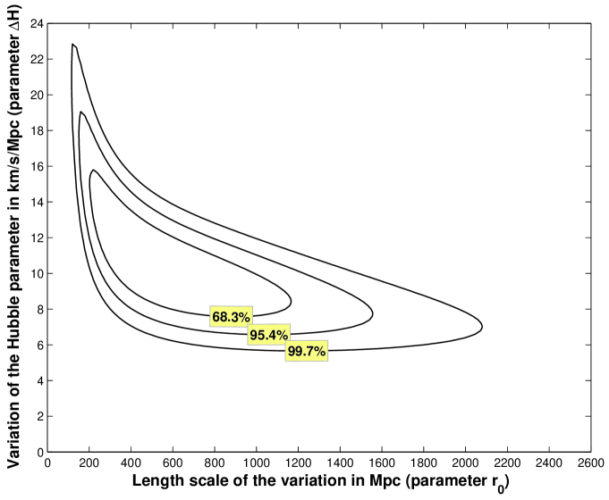
Figure 1: Confidence level contours in the LTB model with $\Omega_{M}(r)={\rm{constant}}=0.45$ and $H_{0}(r)=$ $56.3$ ${\rm{km/s/Mpc}}+\Delta He^{-r/r_{0}}$.

3.2 Inhomogeneous expansion and dust with $\Omega_{M}(r)=1$

The boundary condition functions have here the same form as in the model of Sect. 3.1, but this time we have fixed $\Omega_{M}(r)=1$ in analogy with the flat FRW model. A great virtue of this model is that the scale function can be explicitly solved from Eq. (14). In this case, the best fit values for the parameters are:

• $H+\Delta H=65.5$ ${\rm{km/s/Mpc}}$

• $\Delta H=16.8$ ${\rm{km/s/Mpc}}$

• $r_{0}=1400$ ${\rm{Mpc}}$

• Goodness of the fit: $\chi^{2}=176.3$, $\chi^{2}/157=1.12$

The confidence level contours with $H$ fixed to its best fit value are displayed in Fig. 2. For comparison with the homogeneous case, the best fit flat concordance $\Lambda$CDM model has $\Omega_{M}=0.3$, $\Omega_{\Lambda}=0.7$ and $\chi^{2}=177$, ${\chi^{2}}/{157}=1.13$.

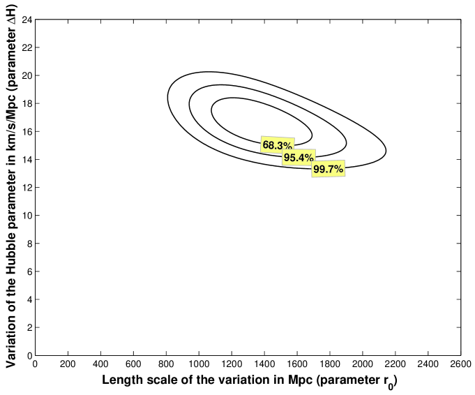
Figure 2: Confidence level contours in the LTB model with $\Omega_{M}(r)={\rm{constant}}=1$ and $H_{0}(r)=$ $48.7$ ${\rm{km/s/Mpc}}+\Delta He^{-r/r_{0}}$.

3.3 Inhomogeneous expansion with $\Omega_{M}(r)+\Omega_{\Lambda}(r)=1$

We have now seen that inhomogeneous models of the universe can fit the supernova data without the cosmological constant. On the other hand, the homogeneous model with the cosmological constant fits the data as well. Thus, it is natural to ask whether an even better fit could be obtained with both the cosmological constant and the inhomogeneities. Let us therefore require that $\Omega_{M}(r)+\Omega_{\Lambda}(r)=1$ with the same form for the function $H_{0}(r)$ as before. Then we find

• $H+\Delta H=66$ ${\rm{km/s/Mpc}}$

• $\Delta H=8$ ${\rm{km/s/Mpc}}$

• $r_{0}=600$ ${\rm{Mpc}}$

• $\Omega_{\Lambda}\equiv\rho_{\Lambda}/\rho_{{\rm{crit}}}=0.33$ for fixed $\rho_{{\rm{crit}}}=3H^{2}/{(8\pi G)}$ with $H=66$ ${\rm{km/s/Mpc}}$

• Goodness of the fit: $\chi^{2}=173.4$, $\chi^{2}/157=1.10$

Comparing this model with the homogeneous flat $\Lambda$CDM ($\chi^{2}/157=1.13$) and the analogous inhomogeneous dust model of Sect. 3.2 ($\chi^{2}/157=1.12$) suggests that the mixture of the inhomogeneous expansion and the vacuum energy does not give a better fit than either of them separately.

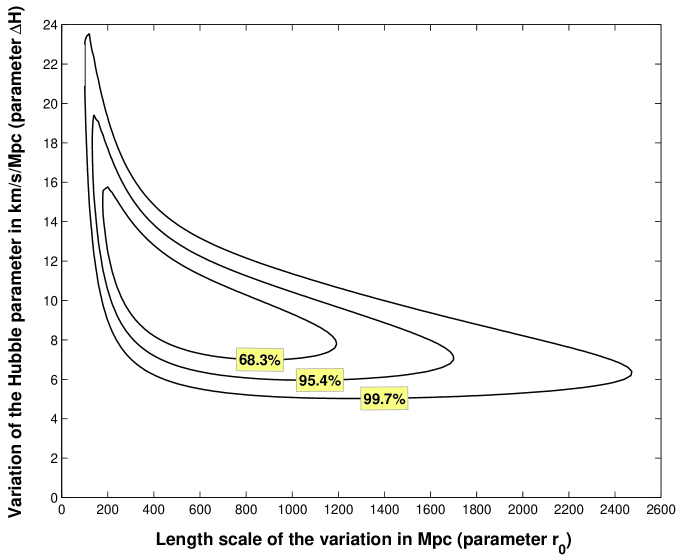
Figure 3: Confidence level contours in the LTB model with perfectly uniform present-day matter density: $H_{0}(r)=57$ ${\rm{km/s/Mpc}}+\Delta He^{-r/r_{0}}$, $\Omega_{M}(r)=0.29(67$ ${\rm{km/s/Mpc}})^{2}/H_{0}^{2}(r)$.

3.4 Inhomogeneous expansion and dust with $\rho_{M}(r,t_{0})={\rm{const.}}$

Let us then consider a model with strictly uniform present-day matter distribution: $\rho_{M}(r,t_{0})={\rm{constant}}$. As can be seen in Eq. (31), the condition for the uniformity is: $H_{0}^{2}(r)\Omega_{M}(r)={\rm{constant}}$. Therefore, we choose the boundary condition functions to be of the form

$$H_{0}(r) = H+\Delta He^{-r/r_{0}}~{},$$

$$\Omega_{M}(r) = \Omega_{0}(H+\Delta H)^{2}/(H+\Delta He^{-r/r_{0}})^{2}~{}.$$ (27)

The data analysis then gives the following best fit values:

• $H+\Delta H=67$ ${\rm{km/s/Mpc}}$

• $\Delta H=10$ ${\rm{km/s/Mpc}}$

• $r_{0}=450$ ${\rm{Mpc}}$

• $\Omega_{0}=0.29$

• Goodness of the fit: $\chi^{2}=172.6$, ${\chi^{2}}/{157}=1.10$

The confidence level contours with $\Omega_{0}$ and $H$ fixed to their best fit values are displayed in Fig. 3.

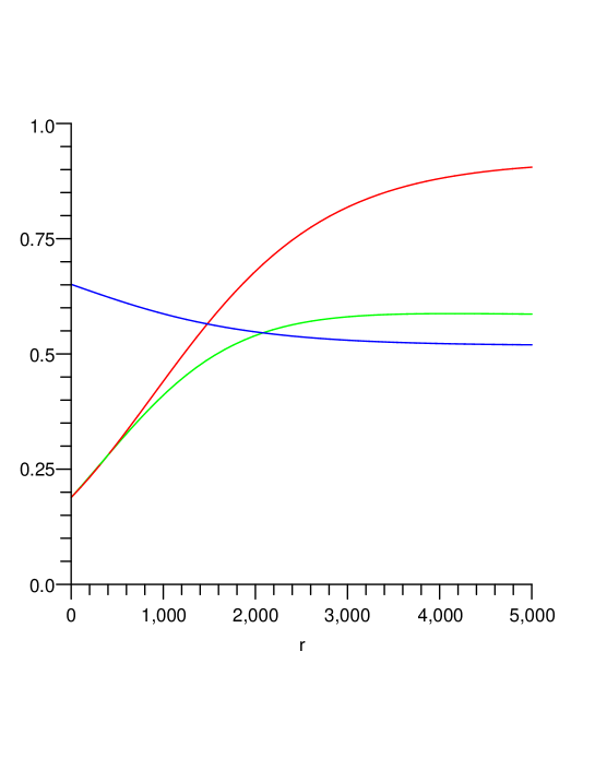
Figure 4: The functions $\Omega_{M}(r)$ (red line), $H_{0}(r)$ in the units of $100$ ${\rm{km/s/Mpc}}$ (blue line) and the physical matter density today $\rho_{M}(r,t_{0})$ in the units of the critical density at the origin $\rho_{{\rm{crit}}}(0)$ (green line) for the best fit values in the model with simultaneous Big Bang.

3.5 Inhomogeneous expansion with simultaneous Big Bang

Finally, let us consider a model with simultaneous Big Bang, i.e. a spatially constant age of the universe (52). This constraint leaves us with only one free function. Hence, to maintain the radially decreasing Hubble expansion, we choose the boundary condition functions to have the form

$$H_{0}(r) = H\left[\frac{\sqrt{1-\Omega_{M}(r)}-\Omega_{M}(r){\rm{arsinh}}\sqrt{\frac{1-\Omega_{M}(r)}{\Omega_{M}(r)}}}{(1-\Omega_{M}(r))^{3/2}}\right]~{},$$

$$\Omega_{M}(r) = \frac{\Omega_{0}}{(1+\delta e^{-r/r_{0}})^{2}}~{}.$$ (28)

The data analysis gives that the best fit values for these parameters are: $H=76.5$ ${\rm{km/s/Mpc}}$, $\delta=1.21$, $r_{0}=1000$ ${\rm{Mpc}}$, $\Omega_{0}=0.92$, goodness of the fit: $\chi^{2}=175.5$, $\chi^{2}/157=1.12$. These values imply that the Hubble function $H_{0}(r)$ varies from the value $H_{0}(0)=65$ ${\rm{km/s/Mpc}}$ near us to its asymptotic value $H_{0}(r\gg r_{0})=52$ ${\rm{km/s/Mpc}}$, as shown in Fig 4. Eq. (52) then gives the age of the universe simply as $t_{{\rm{age}}}=1/H=12.8$ ${\rm{Gyr}}$. The values are similar to the model of Ref. [26].

3.6 Discussion of the fits

As proved by Mustapha, Hellaby and Ellis, any isotropic set of observations can be explained by appropriate inhomogeneities in the LTB model [14]. Hence, the fact that we could find boundary conditions fitting the supernova observations is not surprising. Instead, the novel aspect here is the form of these functions that gives the best fit, as well as their physical interpretation: inhomogeneities in the expansion rate but homogeneous present-day matter density. The particular interest lies in the fact that the analysis is not only in qualitative agreement with the observed homogeneity in galaxy surveys, but also gives a similar value for the present-day matter density: $\Omega_{M}\lesssim 0.4$. Of course, the matter power spectrum should be reanalyzed in the LTB model to confirm the quantitative agreement, but we do not expect a small spatial variation of the Hubble parameter to change the result notably.

Indeed, the smallness ($\sim 15\%$) of the spatial variation in the Hubble parameter is another significant result of the fits in Sects. 3.1 and 3.4. The variation can be considered small, as it is of the same order with the uncertainty of the model-independently deduced value for the local Hubble rate [36]. The variation of the Hubble parameter found by Alnes, Amarzguioui and Grøn [26] has also similar magnitude, but their model contains a large ($\sim 400\%$) variation in the matter density.

In addition to the ones discussed in Sects. 3.1-3.5, we have considered various other forms for the boundary condition functions $\Omega_{M}(r)$ and $H_{0}(r)$. A generic outcome is that inhomogeneities in $H_{0}(r)$ appear to have a much bigger effect on the goodness of the fit than the inhomogeneities in $\Omega_{M}(r)$. In fact, we have been able to obtain good fits for the $H_{0}(r)=H+\Delta He^{-r/r_{0}}$ -models with inhomogeneities of almost any kind on $\Omega_{M}(r)$. Moreover, we have found that models with $H_{0}(r)={\rm{const.}}$ do not give a good fit irrespective of what kind of inhomogeneities we have inserted in $\Omega_{M}(r)$. As an exception, a relatively high ($\Omega_{0}\sim 30$) and thin ($r_{0}\sim 150$ ${\rm{Mpc}}$) peak of the form $\Omega_{M}(r)=\Omega_{0}e^{-r/r_{0}}+\Omega_{0}/(3e^{4})$ seems to slightly improve the fit, giving $\chi^{2}\sim 180$ when $H_{0}(r)={\rm{const.}}$; the result can be understood by looking at Eq. (31), which places the derivatives of the functions $\Omega_{M}(r)$ and $H_{0}(r)$ on a similar position, and as $H_{0}^{\prime}(r)<0$ can mimic acceleration, so can $\Omega_{M}^{\prime}(r)<0$.

The results of Sect. 3.3 indicate that the inhomogeneities of the expansion rate and vacuum energy are mutually exclusive in the sense that their combination does not lead to a better fit. A good fit can be achieved either by having vacuum energy but no inhomogeneities; by having inhomogeneities but no vacuum energy; or by having both about the half amount of their separately deduced best fit values, i.e. they seem to have a very similar effect on the supernova observations.

The early supernova data had a discrepancy between the Hubble parameter deduced from the low redshift sample and the one deduced from the high redshift sample [37], but it seems to have vanished from the latest supernova data [38]. However, the results of Sects. 3.1-3.5 suggest that the feature still exists, and rather than a discrepancy in the data, it is actually an alternative explanation to dark energy. Note that the LTB model certainly describes a universe with spatially varying expansion rate more realistically than two separate FRW models, one for high redshift regime and another for low redshifts. In addition, the discrepancy in the early supernova data between the local and global Hubble parameters had a similar magnitude with our best fit value for the variation of the Hubble parameter. The length scale associated with the variation of the Hubble parameter, found to lie within the range of about $200$ to $1200$ ${\rm{Mpc}}$ in our analysis, matches the explanation as well.

As can be seen in Sect. 3.2, the explicitly solvable LTB model with $\Omega_{M}(r)=1$ fits the data essentially as well as the more complicated ones with $\Omega_{M}(r)\neq 1$. Hence it will be a useful example when discussing the time evolution of the inhomogeneities in Sect. 3.7 and the average expansion in Sect. 4.

In order to respect the cosmological principle, we should not live in the dead center of a region that is expanding faster than the global average. It was shown in [39] that the supernova data does not impose severe restrictions for the location of an off-center observer, but as argued in [34], perhaps the most relevant constraint comes from the dipole anisotropy of the CMB. Here we give a rough estimate for the off-center distance allowed by the CMB dipole.

We define the effective peculiar velocity, caused by the inhomogeneous expansion, that an observer at the coordinate $r=d$ has relative to the symmetry center

$$v_{p}(d)=d(H_{0}(0)-H_{0}(d)),$$ (29)

which simply measures the deviation from the Hubble law. In a homogeneous universe, the effective peculiar velocity of Eq. (29) is identically zero and the observed peculiar velocity is accounted for motion relative to the comoving coordinates. We instead assume this coordinate velocity negligible and require that the effective peculiar velocity of Eq. (29) gives rise to the CMB dipole. Inserting the velocity deduced from the CMB dipole, $v_{p}=370$ ${\rm{km/s}}$ [40], and the boundary condition function $H_{0}(r)$ of Eq. (3.4) with the best fit values $r_{0}=450$ ${\rm{Mpc}}$, $\Delta H=10$ ${\rm{km/s/Mpc}}$ to Eq. (29) gives $d=140$ ${\rm{Mpc}}$, which is somewhat more than was found in a more thorough analysis for a different model [34]. This is a non-negligible fraction of the size of the inhomogeneity, $d/r_{0}=0.3$, so according to this naive estimate the CMB dipole does not constrain our position strictly to the center. Of course even greater off-center distances are allowed if we would also have coordinate velocity in the opposite direction to counterbalance the effective peculiar velocity of Eq. (29).

3.7 Time evolution of the inhomogeneities

In the preceding discussion we defined the models by giving the boundary conditions $H_{0}(r)$ and $\Omega_{M}(r)$ on the present-day spatial hypersurface. However, as is inherent in the Big Bang cosmology, the question of the ”naturalness” of the initial conditions arises in models with inhomogeneous expansion but a homogeneous present-day matter distribution. In this section, we address the problem by considering the time evolution of the inhomogeneities in the explicitly solvable LTB model with $\Omega_{M}(r)=1$. We expect the same qualitative features to hold in the more general case with $\Omega_{M}(r)\lesssim 1$ as well. For more on the subject, see e.g. [9].

Combining Eqs. (6) and (10) we obtain the following expression for the matter density:

$$\rho_{M}(r,t)=\rho_{M}(r,t_{0})\left(\frac{A_{0}^{2}(r)A_{0}^{\prime}(r)}{A^{2}(r,t)A^{\prime}(r,t)}\right)~{},$$ (30)

where

$$\rho_{M}(r,t_{0})=\frac{3H_{0}^{2}(r)}{8\pi G}\Omega_{M}(r)\left[1+\frac{A_{0}(r)}{3A_{0}^{\prime}(r)}\left(\frac{\Omega_{M}^{\prime}(r)}{\Omega_{M}(r)}+2\frac{H_{0}^{\prime}(r)}{H_{0}(r)}\right)\right]~{}.$$ (31)

With $\Omega_{M}(r)=1$ and $A_{0}(r)=r$, Eq. (30) reduces to

$$\rho_{M}(r,t)=\frac{3H_{0}^{2}(r)+2rH_{0}^{\prime}(r)H_{0}(r)}{8\pi G[1+\frac{3H_{0}(r)}{2}(t-t_{0})][r(t-t_{0})H_{0}^{\prime}(r)+(1+\frac{3H_{0}(r)}{2}(t-t_{0}))]}~{},$$ (32)

which gives the explicit time dependence of the matter distribution. Using Eq. (32), one finds that the ratio of the matter density near us ($r=0$) to its asymptotic value ($r=R\gg r_{0}$) is

$$\frac{\rho_{M}(0,t)}{\rho_{M}(R,t)}=\left[\frac{H_{0}(0)}{H_{0}(R)}\frac{\left(1+\frac{3}{2}H_{0}(R)(t-t_{0})\right)}{\left(1+\frac{3}{2}H_{0}(0)(t-t_{0})\right)}\right]^{2}~{}.$$ (33)

At late times, $t=T\gg t_{0}$, Eq. (33) gives

$$\frac{\rho_{M}(0,T)}{\rho_{M}(R,T)}\longrightarrow 1~{},$$ (34)

which means that, irrespective of the initial conditions, the homogeneity of the matter distribution is an attractor solution.

By performing the integral of Eq. (14), one can calculate the explicit time dependence of the expansion rate:

$$H(r,t)=\frac{H_{0}(r)}{1+\frac{3H_{0}(r)}{2}(t-t_{0})}~{}.$$ (35)

Eq. (35) gives the ratio of the local ($r=0$) and global ($r=R\gg r_{0}$) Hubble parameters

$$\frac{H(0,t)}{H(R,t)}=\frac{H_{0}(0)}{H_{0}(R)}\frac{\left(1+\frac{3}{2}H_{0}(R)(t-t_{0})\right)}{\left(1+\frac{3}{2}H_{0}(0)(t-t_{0})\right)}~{},$$ (36)

which tells us that the inhomogeneity of the expansion rate will also vanish in the late ($t=T\gg t_{0}$) universe:

$$\frac{H(0,T)}{H(R,T)}\longrightarrow 1~{}.$$ (37)

By comparing Eqs. (33) and (36) one sees that the inhomogeneity of the matter density will diminish more rapidly than the inhomogeneity of the expansion rate. This explains in a natural way why, with generic initial conditions, the present universe would have negligible inhomogeneities in the matter distribution but detectable inhomogeneities in the expansion rate, like our best fit model in Sect. 3.4. On the other hand, as noted in Sect. 3.6, even if today’s variations in the matter density were of the same order with the required small variation in the expansion rate, the observations might not be able to detect them.

Turning the argument around, Eqs. (33) and (36) tell us that in order to have noticeable inhomogeneities today, the early universe should have been very inhomogeneous. Naturally, we do not have an explanation for this as there is no theory that would determine the initial conditions of the universe. However, when considering the backward time evolution, one should keep in mind that the dust approximation will break down at some stage and as a consequence, Eqs. (32) and (35) do not represent the inhomogeneities of the very early universe.

3.8 The age of the universe

The age of the perfectly homogeneous universe is a well-defined number, the difference $t_{{\rm{age}}}\equiv t_{0}-t_{BB}$ of the time coordinate today $t_{0}$ and the time coordinate for which the scale function goes to zero $a(t\rightarrow t_{BB})\rightarrow 0$. However, with inhomogeneities the notion of the age of the universe becomes more complicated as the age can depend on the spatial location (see e.g. [9]). In the LTB model this can be seen by noting that the singularity condition $A(r,t_{BB})=0$ now defines a curve $t_{BB}(r)$ on the $(r,t)$-plane whereas in the homogeneous FRW case $a(t_{BB})=0$ defines a unique point $t_{BB}$ on the $t$-axis. We give the explicit expressions of the age of the LTB universe as a function of the boundary conditions $H_{0}(r)$ and $\Omega_{M}(r)$ for different cases in Appendix A.

The expressions (52), (53), (54) and (55) are similar to the homogeneous FRW case, except for the $r$-dependence. In this case, the local value of the Hubble parameter gives the order of magnitude for the local age of the universe. Thus, if $\Omega_{M}(r)={\rm{const.}}$, already small spatial fluctuations in the Hubble parameter $H_{0}(r)$ lead to quite big variations in the age of the universe between different spatial locations. For a constant $\Omega_{M}(r)$ the scale of the spatial variation in the age of the universe is simply given by $(\Delta H)^{-1}$, and at scales of ${\cal O}(1000)$ ${\rm{Mpc}}$ would thus be some billions of years for the best fit models of Sects. 3.1-3.4. Although theoretically inhomogeneous Big Bang could be a viable possibility (one need only to think of e.g. colliding branes; see [41, 42]), age differences of such great magnitude could be hard to reconcile with any existing model of the very early universe. They certainly contradict the spirit of inflation, where the whole observable universe arises from a single causal domain. However, the possibility remains that, for some reason, $H_{0}(r)$ and $\Omega_{M}(r)$ are related in such a fashion that they give $t_{{\rm{age}}}(r)={\rm{constant}}$. The inhomogeneous LTB model would continue to fit the supernova data well as demonstrated by the model of Sect. 3.5.

4 Is accelerated average expansion needed?

The expansion of the dust dominated LTB universe does not accelerate anywhere but nevertheless can, as shown e.g. in Sect. 3, fit the supernova observations. However, it has been argued that a certain kind of average expansion can accelerate even though the local expansion would decelerate everywhere [13, 16, 18]. The aim in this section is to study if this kind of average acceleration appears in our best fit models of Sect. 3. For this purpose, we need the Buchert equations that describe the averaged dynamics of a general irrotational dust universe [16]

$$3\frac{\ddot{a}(t)}{a(t)}=-4\pi G\langle\rho_{M}\rangle_{D}+\frac{2}{3}(\langle\theta^{2}\rangle_{D}-\langle\theta\rangle_{D}^{2})-\langle\sigma^{\mu\nu}\sigma_{\mu\nu}\rangle_{D}$$ (38)

$$3\frac{\dot{a}^{2}(t)}{a^{2}(t)}=8\pi G\langle\rho_{M}\rangle_{D}-\frac{1}{2}\langle R^{(3)}\rangle_{D}-\frac{1}{3}(\langle\theta^{2}\rangle_{D}-\langle\theta\rangle_{D}^{2})+\frac{1}{2}\langle\sigma^{\mu\nu}\sigma_{\mu\nu}\rangle_{D}$$ (39)

$$\frac{\partial}{\partial t}\langle\rho_{M}\rangle_{D}+3\frac{\dot{a}(t)}{a(t)}\langle\rho_{M}\rangle_{D}=0~{},$$ (40)

where $\sigma^{\mu\nu}\sigma_{\mu\nu}\geq 0$ represents the shear, $a(t)\equiv(\int_{D}\sqrt{{\rm{det}}[g_{ij}]}d^{3}x)^{1/3}$ is the averaged scale factor, $D$ is the integration domain, $g_{ij}$ is the spatial part of the metric, $R^{(3)}$ is the curvature scalar of the $t={\rm{const.}}$ spatial hypersurface, $\theta\equiv\nabla_{\mu}u^{\mu}$ is the expansion scalar and the spatial average of a scalar $S$ is defined as

$$\langle S\rangle_{D}\equiv\frac{\int_{D}S\sqrt{{\rm{det}}[g_{ij}]}d^{3}x}{\int_{D}\sqrt{{\rm{det}}[g_{ij}]}d^{3}x}~{}.$$ (41)

The difference of Buchert’s acceleration equation (38) and its homogeneous FRW counterpart is known as the backreaction

$$Q\equiv\frac{2}{3}(\langle\theta^{2}\rangle_{D}-\langle\theta\rangle_{D}^{2})-\langle\sigma^{\mu\nu}\sigma_{\mu\nu}\rangle_{D}~{}.$$ (42)

The average expansion accelerates if the right hand side of Eq. (38) is positive; this can be achieved by having large enough variance of the expansion rate although it is counterbalanced by the average shear. The variance gets large values when contracting ($\theta<0$) and expanding ($\theta>0$) regions coexist, and in fact the average acceleration has been connected to gravitational collapse [13, 33]. However, as demonstrated in [43], a globally expanding dust universe can have average acceleration as well.

The definition of the shear tensor is

$$\sigma_{\mu\nu}\equiv\frac{1}{2}(\nabla_{\mu}u_{\nu}+\nabla_{\nu}u_{\mu})-\frac{1}{3}(g_{\mu\nu}+u_{\mu}u_{\nu})\nabla_{\alpha}u^{\alpha}~{},$$ (43)

where $u^{\mu}$ is the four-velocity of the dust. Calculating the shear and the expansion scalar for the LTB metric in the coordinates of Eq. (1) gives

$$\sigma^{\mu\nu}\sigma_{\mu\nu}=\frac{2}{3}\left(\frac{\dot{A}}{A}-\frac{\dot{A}^{\prime}}{A^{\prime}}\right)^{2}$$ (44)

$$\theta=2\frac{\dot{A}}{A}+\frac{\dot{A}^{\prime}}{A^{\prime}}\equiv 2H(r,t)+H_{r}(r,t)~{}.$$ (45)

Using the field equation (5) one finds that the two Hubble functions $H(r,t)$ and $H_{r}(r,t)$, defined in Eq. (45), are related at the present time $t_{0}$ as

$$H_{r}(r,t_{0})=H_{0}(r)+rH_{0}^{\prime}(r)~{},$$ (46)

so that at $t=t_{0}$ the shear and the expansion rate have the expressions

$$\sigma^{\mu\nu}\sigma_{\mu\nu}(t=t_{0}) = \frac{2}{3}(rH_{0}^{\prime}(r))^{2}$$

$$\theta(t=t_{0}) = 3H_{0}(r)+rH_{0}^{\prime}(r)~{}.$$ (47)

Inserting Eqs. (3.4) and (4) to Buchert’s acceleration equation (38), we obtain the exact expression for the average acceleration of the model in Sect. 3.4:

$$3\frac{\ddot{a}(t_{0})}{a(t_{0})}=-\frac{3}{2}\Omega_{0}H^{2}+6\langle H_{0}^{2}\rangle+4\langle rH_{0}^{\prime}H_{0}\rangle-6\langle H_{0}\rangle^{2}-4\langle rH_{0}^{\prime}\rangle\langle H_{0}\rangle-\frac{2}{3}\langle rH_{0}^{\prime}\rangle^{2}~{}.$$ (48)

We choose the integration domain in Eq. (48) as the origin-centered ball with radius $R$, taken to be greater than the inhomogeneity scale (e.g. $R\approx 2r_{0}$) but smaller than the horizon distance $R<1/H$. Note that at $t=t_{0}$ we have $\sqrt{{\rm{det}}[g_{ij}]}=r^{2}/\sqrt{1-k(r)}$ in the integration measure. As the curvature function of Eq. (11) is small for the models of Sect. 3, we can make the linear approximation, $1/\sqrt{1-k(r)}\approx 1+k(r)/2$, for the integrals in Eq. (41) to get an approximate expression for the average of a scalar $S$

$$\langle S\rangle_{\mathbb{B}(R)}\equiv\frac{\int_{0}^{R}Sr^{2}(1-k(r))^{-1/2}dr}{\int_{0}^{R}r^{2}(1-k(r))^{-1/2}dr}\approx\langle S\rangle_{c}+\frac{1}{2}\langle Sk\rangle_{c}-\frac{1}{2}\langle S\rangle_{c}\langle k\rangle_{c}~{},$$ (49)

where we have used $\langle S\rangle_{c}$ to denote the ”coordinate” average:

$$\langle S\rangle_{c}\equiv\frac{\int_{0}^{R}Sr^{2}dr}{\int_{0}^{R}r^{2}dr}~{}.$$ (50)

Using the approximation of Eq. (49), we can calculate the integrals of Eq. (48) to obtain an expression for the average acceleration of the model in Sect. 3.4:

$$\begin{split}\frac{3}{r_{0}^{2}H^{4}}\frac{\ddot{a}(t_{0})}{a(t_{0})}=-\frac{3\Omega_{0}}{2r_{0}^{2}H^{2}}+\bigg{(}\frac{64}{81}h^{2}+\frac{9}{2}h-288(1-\Omega_{0})\bigg{)}\frac{h^{2}}{x^{3}}e^{-x}\\ +\bigg{(}\frac{6}{5}(1-\Omega_{0})x^{2}+9(1-\Omega_{0})x+135(1-\Omega_{0})\frac{1}{x}+279(1-\Omega_{0})\frac{1}{x^{2}}\\ -\frac{27}{4}\frac{h^{2}}{x^{3}}-432\frac{h}{x^{3}}+\frac{567}{2}(1-\Omega_{0})\frac{1}{x^{3}}+42(1-\Omega_{0})\bigg{)}h^{2}e^{-2x}\\ +\bigg{(}2x^{2}+\frac{43}{3}x+\frac{1855}{9}\frac{1}{x}+\frac{11405}{27}\frac{1}{x^{2}}+\frac{69223}{162}\frac{1}{x^{3}}+\frac{586}{9}\bigg{)}h^{3}e^{-3x}\\ +\bigg{(}\frac{1}{2}x^{2}+\frac{53}{24}x+\frac{2945}{288}\frac{1}{x}+\frac{19475}{1728}\frac{1}{x^{2}}+\frac{124313}{20736}\frac{1}{x^{3}}+\frac{419}{72}\bigg{)}h^{4}e^{-4x}\\ -\frac{9}{256}\frac{h^{4}}{x^{3}}+\frac{16}{81}\frac{h^{3}}{x^{3}}+\frac{9}{2}(1-\Omega_{0})\frac{h^{2}}{x^{3}}~{},\end{split}$$ (51)

where we have denoted $h\equiv\Delta H/H$ and $x\equiv R/r_{0}$. A careful inspection reveals that the negative first term on the right hand side of Eq. (51) dominates, at least for the values of the parameters $r_{0}$, $\Delta H$, $H$ and $\Omega_{0}$ that give a good fit. Thus, according to Eq. (51), the average expansion does not accelerate in the best fit model of Sect. 3.4. The validity of Eq. (51) is verified by the fact that it actually deviates only about $10^{-7}$ from the numerically computed accurate result of the integrals in Eq. (48) for the best fit values $h=10/57$, $r_{0}=450$ ${\rm{Mpc}}$ and $\Omega_{0}=0.4$. We have repeated the computation of the average expansion also for the model of Sect. 3.1 and found no acceleration there either.

Finally, let us consider the LTB model with $\Omega_{M}(r)=1$. For this model, both the backreaction of Eq. (42) and the 3-curvature $R^{(3)}$ vanish identically [43]. Thus, the Buchert equations (38), (39) and (40) reduce to the FRW equations of the flat and homogeneous dust universe. However, a creature living in the LTB universe would observe the luminosity-redshift relation calculated from the exact Einstein equations, not from the FRW equations. The difference between these results is significant since, as shown in Sect. 3.2, the LTB model with $\Omega_{M}(r)=1$ fits the supernova observations whereas the flat matter dominated FRW model does not [2]. As the averaged matter density $\langle\rho_{M}\rangle_{D}$ has only a small dependence on the averaging domain $D$ in our models, the conclusion would not change even if one were to use a different smoothing scale $R_{i}$ for every supernova at $r=R_{i}$. Overall, there seems to be no meaningful way of using the averaged equations to calculate the actual observables, e.g. the luminosity-redshift relation.

5 Conclusions

We have studied the effect of inhomogeneities on the cosmological supernova observations in the spherically symmetric matter dominated LTB universe. Our main conclusions are as follows:

1. The inhomogeneous matter dominated LTB model fits the supernova data better than the homogeneous FRW model with the cosmological constant.

2. Inhomogeneities of the expansion rate seem to have much bigger effect on the goodness of the fit than the inhomogeneities of the matter distribution.

3. The model giving the best fit has perfectly uniform present-day matter density with $\Omega_{M}\sim 0.3$, in agreement with the galaxy surveys, but its Hubble parameter varies from the local value of $\sim 70$ ${\rm{km/s/Mpc}}$ to the value of $\sim 60$ ${\rm{km/s/Mpc}}$ over the distance scale of $\sim 500$ ${\rm{Mpc}}$ from us.

4. Neither local nor average acceleration is needed for a good fit to the supernova data.

5. At least in the LTB universe, the averaged Buchert equations give a notably different prediction for the observable luminosity-redshift relation than the exact Einstein equations.

The first of the above listed results is neither new nor surprising, as it was proved in [14] that any isotropic set of observations can be explained by appropriate inhomogeneities, and later demonstrated with examples by several authors. Instead, the second result is a new one, as is the model that explains both the observations of supernovae and the observed homogeneity in the large scale distribution of galaxies without invoking dark energy. Moreover, we found in Sect. 3.7 that within the dynamics of the Einstein equation, the universe may evolve to this kind of a configuration without any substantial amount of fine-tuning in the initial conditions. In addition, as the supernovae and galaxy surveys constrain the boundary condition functions $H_{0}(r)$ and $\Omega_{M}(r)$ only for the small values of the radial coordinate $r$, the tails of these functions can still be freely chosen to give a good fit for the CMB power spectrum as well. In fact, Alnes, Amarzguioui and Grøn have realized this in practice by fitting the LTB model to the first peak of the CMB [26]. It has also been shown that even a homogeneous model can fit the CMB data without dark energy [44].

Our another focus was on the averaged dynamics of the dust universe, given by the Buchert equations that illustratively demonstrate the potential cosmological significance of the inhomogeneities. In Sect. 4, we showed that none of our dust models that fit the supernova observations have accelerated average expansion. On the other hand, one can easily construct examples that have average acceleration but are ruled out by observations, whereas dust models that would both have the average acceleration and fit the cosmological data are still to be presented. Moreover, as discussed at the end of Sect. 4, it seems that the Buchert equations cannot be used to calculate the observable luminosity-redshift relation. Although explicitly demonstrated only in the LTB universe, we expect that it might be the case in the more general models as well; after all, the Buchert equations are obtained by integrating over a spatial hypersurface whereas the observables are calculated by integrating over the past light cone. Altogether, averaging over a spatial hypersurface is perhaps not practical if one wants to make comparison with the observations. Instead, probably a better alternative is to relate the inhomogeneities directly to the observations, as done e.g. in this paper and, if needed, take the averages only of the relevant observables, such as the energy flux and redshift of light.

Of course, some sort of smoothing is implicitly assumed also in the LTB model. Therefore, the study of observations in the LTB universe does not answer the interesting question about the potential cosmological consequences of the small scale lumpiness caused by galaxies. Their effect could be significant, possibly depending also on how smoothly dark matter, perhaps the dominant energy component of the universe, is distributed in the universe.

Appendix A The age of the LTB universe

The age of the LTB-universe can be calculated by integrating the field equation (12). In the cases where the result is an elementary function of the boundary conditions, the results are:

1. $\Omega_{M}(r)<1$ and $\Omega_{\Lambda}(r)=0$:

   $$t_{{\rm{age}}}(r)=\frac{\sqrt{1-\Omega_{M}(r)}-\Omega_{M}(r){\rm{arsinh}}\sqrt{\frac{1-\Omega_{M}(r)}{\Omega_{M}(r)}}}{H_{0}(r)(1-\Omega_{M}(r))^{3/2}}~{}.$$ (52)

2. $\Omega_{M}(r)>1$ and $\Omega_{\Lambda}(r)=0$:

   $$t_{{\rm{age}}}(r)=\frac{\Omega_{M}(r){\rm{arcsin}}\sqrt{\frac{\Omega_{M}(r)-1}{\Omega_{M}(r)}}-\sqrt{\Omega_{M}(r)-1}}{H_{0}(r)(\Omega_{M}(r)-1)^{3/2}}~{}.$$ (53)

3. $\Omega_{M}(r)=1$ and $\Omega_{\Lambda}(r)=0$:

   $$t_{{\rm{age}}}(r)=\frac{2}{3H_{0}(r)}~{}.$$ (54)

4. $\Omega_{M}(r)+\Omega_{\Lambda}(r)=1$:

   $$t_{{\rm{age}}}(r)=\frac{2}{3H_{0}(r)}\frac{{\rm{arsinh}}\sqrt{\frac{1-\Omega_{M}(r)}{\Omega_{M}(r)}}}{\sqrt{1-\Omega_{M}(r)}}~{}.$$ (55)