On the stability of accelerating relativistic shock waves

Abstract

We consider the corrugation instability of the self–similar flow with an accelerating shock in the highly relativistic regime. We derive the correct dispersion relation for the proper modes in the self–similar regime, and conclude that this solution is unstable.

1 Introduction

It has long been known that the propagation of a shock through the outer layers of a star may, for sufficiently steep density distributions, lead to shock acceleration. Self–similar solutions (Gandel’man and Frank-Kamenetskii 1956, Sakurai 1960, Raizer 1964, Grover and Hardy 1966, Hayes 1968) notoriously provide excellent approximations to the generic solutions, for a reason most clearly discussed by Raizer (1964): behind the shock, a sonic point is formed, which prevents causal connection between the region immediately behind the shock with the more distant regions, which are sensitive to boundary conditions. Disconnection from initial conditions limits the number of parameters on which the solution may depend, while still allowing the existence of a self–similar solution. Because of the independence from initial conditions, it is expected that, shortly after their formation, all solutions with accelerating shocks will quickly approach the self–similar solution.

Because of the possible relevance of these solutions to the evolution of Gamma Ray Bursts, there has been recently a strong surge of interest in their properties, especially in the relativistic regime, which, at least asymptotically, should be most appropriate to GRBs. A highly relativistic, self–similar solution has been presented by Perna and Vietri (2002) in planar geometry, for which accelerating, self–similar solutions appear for exponentially decreasing density stratifications outside the star. In spherical geometry, it is instead possible to find a richer spectrum of self–similar solutions, for basically any type of power–law density stratification (Best and Sari 2000, Pan and Sari 2005, Sari 2005). These solutions are often referred to as Type II solutions (Barenblatt 1996), meaning that the behaviour of the full solution cannot be determined from dimensional analysis alone, like in the well–known Sedov solution, but is fixed instead by the conditions of regularity at some particularly difficult point, like the sonic point.

The stability of relativistic hydrodynamic solutions with shocks is rarely considered in the literature. Gruzinov (2001) considered the linear stability of the spherically symmetric, relativistic explosions of Blandford and McKee (1976), but nothing is currently known about the stability of accelerating solutions, in the relativistic regime. In the Newtonian regime, the self–similar solutions are known to be unstable, from both a linear analysis (Chevalier 1990), and a numerical, non–linear one (Luo and Chevalier 1994). The relativistic solutions differ from this analysis in two distinct respects: on the one hand, they include relativistic effects, on the other one, since the shock is supposed to be highly relativistic, they are obliged to assume the validity of the ultra–relativistic equation of state, $p=e/3$. Both of these circumstances lead to a greater susceptibility to corrugational instabilities. In fact, softening the equation of state leads to corrugational instability even for shocks propagating into a constant density environment: Ryu and Vishniac (1987) found a range of instabilities provided the adiabatic index is $\gamma\lesssim 1.2$. Also, assuming an adiabatic index close to $\gamma=5/3$ leads to both a narrower instability range in the parameter $k$, and in smaller growth rates than determined by Chevalier (1990) for $\gamma=4/3$ in the Newtonian, accelerating self–similar flow (Vietri, unpublished).

On the other hand, relativistic effects tend to make pressure waves slow when compared to bulk motion, and thus to decouple nearby layer of fluid. Thus, if a purely kinematic difference exists in the motion of adjacent layers, it is more likely to grow because of the lack of restoring effects.

The plan of this paper is as follows. In the next section, we shall briefly summarize the properties of the zero–th order solution of Perna and Vietri (2002). In the following section we shall perform a linear stability analysis, showing that accelerating, self–similar shocks are indeed unstable. In the last section, we shall discuss our results.

2 The unperturbed solution

Here we briefly recall the relevant properties of the zero–th order solution. The self–similar solution for an accelerating hyperrelativistic shock wave in a planar exponential atmosphere, in the highly relativistic regime, was derived by Perna and Vietri (2002). In their notation, the ambient density is given by

$$\rho(x)=\rho_{0}e^{-k_{0}x},$$ (1)

where $\rho_{0}$ and $k_{0}$ are constants. If $X^{i}(s)$ denotes the shock position at proper time $s$, dimensional and covariance arguments impose

$$\frac{dX^{i}}{ds}=\frac{\alpha k^{i}}{k_{\mu}k^{\mu}s},\qquad i\in\left\{1,2,3\right\},$$ (2)

where $k_{\mu}\equiv(0,k_{0},0,0)$ in the upstream frame and $\alpha$ is a dimensionless (negative) constant to be determined by imposing a smooth passage of the flow through a critical point.

Integrating (2), it follows that

$$\frac{k_{0}t}{-\alpha}=\log\left(\frac{1+V}{1-V}\right)^{1/2}-\frac{1}{V}+\textrm{const},$$ (3)

whose hyperrelativistic limit is

$$\frac{k_{0}(t-t_{\textrm{i}})}{-\alpha}\approx\log\frac{\Gamma}{\Gamma_{\textrm{i}}}$$ (4)

($V$ denotes the shock speed, $\Gamma$ its Lorentz factor and the subscript i refers to the initial condition). Moreover, from (1),

$$\frac{\Gamma_{\textrm{f}}}{\Gamma_{\textrm{i}}}\approx\left(\frac{\rho_{\textrm{f}}}{\rho_{\textrm{i}}}\right)^{1/\alpha}.$$ (5)

In order to determine the value of $\alpha$, the exact adiabatic fluid flow equations,

$$\left\{\begin{array}[]{l}T^{\mu\nu}_{\quad;\nu}=0\\ (n^{\prime}u^{\mu})_{;\mu}=0\end{array}\right.$$ (6)

($T^{\mu\nu}=wu^{\mu}u^{\nu}-pg^{\mu\nu}$ is the energy-momentum tensor, $w$ and $p$ being respectively local proper enthalpy density and pressure, $u^{\mu}$ is the fluid four-speed and $n^{\prime}$ is the baryon number density as measured in the comoving frame) (Landau and Lifshitz, 1989), are considered in their highly relativistic limit given by

$$\frac{D}{Dt}\frac{e^{3}}{n^{\prime 4}}=0;$$ (7)

$$4\gamma^{2}e\frac{D{\mbox{\boldmath{${v}$}}}}{Dt}+\left({\mbox{\boldmath{${\nabla}$}}}e+{\mbox{\boldmath{${v}$}}}\frac{\partial e}{\partial t}\right)=0;$$ (8)

$$\frac{\partial n}{\partial t}+{\mbox{\boldmath{${\nabla}$}}}\cdot(n{\mbox{\boldmath{${v}$}}})=0;$$ (9)

here ${v}$ and $\gamma$ are respectively the fluid speed and Lorentz factor, and $e=3p=3w/4$ is local proper energy density, where use of the relativistic equation of state, $p=e/3$ has been made, as appropriate in the limit of highly relativistic motion. The operator $D/Dt$ is the usual convective derivative, and $n\equiv n^{\prime}\gamma$ is the baryon number density as seen from the upstream frame, the comoving density being $n^{\prime}$.

The hyperrelativistic limit of Taub’s jump conditions across a planar shock, with vanishing speed parallel to the shock surface, is given by

$$n_{2}=2\Gamma^{2}n_{1},\quad\gamma_{2}^{2}=\frac{1}{2}\Gamma^{2},\quad e_{2}=2\Gamma^{2}w_{1},$$ (10)

where the subscripts 1 and 2 respectively refer to immediately pre- and post-shock quantities (Landau and Lifshitz, 1989). Upstream matter is obviously cold in this limit, since its sound speed obeys $c_{s}\ll c$; thus, using $p_{1}\ll e_{1}\approx\rho_{1}$, from (5) it follows that

$$e_{2}=2\frac{\rho_{0}}{\Gamma_{\textrm{i}}^{\alpha}}\Gamma^{2+\alpha}\equiv 2q_{0}\Gamma^{2+\alpha}$$ (11)

and

$$n_{2}=2\frac{n_{0}}{\Gamma_{\textrm{i}}^{\alpha}}\Gamma^{2+\alpha}\equiv 2z_{0}\Gamma^{2+\alpha},$$ (12)

where $n_{0}\equiv\rho_{0}/m$.

Adopting as self-similarity variable

$$\xi=k_{0}(x-X(t))\Gamma^{2}(t),$$ (13)

the equations (10), (11) and (12) can be cast into self–similar form by means of the definitions:

$$\gamma^{2}(x,t)=g(\xi)\Gamma^{2}(t),\quad e(x,t)=q_{0}R(\xi)\Gamma^{2+\alpha}(t),\quad n(x,t)=z_{0}N(\xi)\Gamma^{2+\alpha}(t),$$ (14)

with

$$g(0)=\frac{1}{2},\quad R(0)=2,\quad N(0)=2.$$ (15)

Substituting (13) and (14) into  (7), (8) and (9) it is possible to write equations for $g$, $R$ and $N$ in the form of a Cauchy problem with ordinary derivatives (the prime stands for the first derivative with respect to $\xi$):

$$R^{\prime}=\frac{2g\left[-2\alpha(4+\alpha)+(2+\alpha)(\alpha-4\xi)g\right]R}{\alpha^{2}+(\alpha-4\xi)g\left[-4\alpha+(\alpha-4\xi)g\right]}$$ (16)

$$g^{\prime}=\frac{g^{2}\left[4(\alpha-4\xi)g-14\alpha-3\alpha^{2}\right]}{\alpha^{2}+(\alpha-4\xi)g\left[-4\alpha+(\alpha-4\xi)g\right]}$$ (17)

$${}N^{\prime}=\frac{Ng\left\{\alpha^{2}(18+5\alpha)+2(\alpha-4\xi)g\left[-2\alpha(5+2\alpha)+(2+\alpha)(\alpha-4\xi)g\right]\right\}}{-\alpha^{3}+(\alpha-4\xi)g\left\{5\alpha^{2}+(\alpha-4\xi)g\left[-5\alpha+(\alpha-4\xi)g\right]\right\}}.$$ (18)

2.1 Analytical solution

At the referee’s request, we show here how to obtain a (nearly complete) analytical solution, which may perhaps prove useful.

First of all, we determine $\alpha$, by demanding the simultaneous vanishing of the numerators and of the denominator of eqs. 16 and 17. We find:

$$\alpha=-(2+4/\sqrt{3})\approx-4.309401\;.$$ (19)

Now we introduce a more convenient quantity,

$$Y\equiv(\alpha-4\xi)g(\xi)\;,$$ (20)

for which we know both the value at the shock front, $Y_{0}$, and at the critical point $Y_{c}$ (from the vanishing of the numerator of eq. 16, for instance):

$$Y_{0}=\frac{\alpha}{2}\;,\;\;\;Y_{c}=\alpha(2-\sqrt{3})\;.$$ (21)

From eq. 17 we also derive the following differential equation for $Y$:

$$Y^{\prime}=\frac{Y}{\alpha-4\xi}\frac{(2\alpha-3\alpha^{2})Y-4\alpha^{2}}{\alpha^{2}+Y^{2}-4\alpha Y}\;,$$ (22)

which can easily be integrated to yield the solution in implicit form:

$${}\alpha-4\xi=\alpha\exp I_{1}\;,\;\;I_{1}\equiv-4\int_{\alpha/2}^{y}\frac{d\!Y}{Y}\frac{\alpha^{2}+Y^{2}-4\alpha Y}{(2\alpha-3\alpha^{2})Y-4\alpha^{2}}\;,$$ (23)

where suitable boundary conditions at the shock ($\xi=0$) have already been inserted. We also find:

$${}I_{1}=f_{1}(y)-f_{1}(\alpha/2)\;,\;\;\;f_{1}(y)=\frac{4}{\alpha}\left(\frac{y}{3\alpha-2}+\frac{\alpha}{4}\ln y-\frac{3\alpha(-4+12\alpha+3\alpha^{2})\ln(4\alpha-2y+3\alpha y)}{4(3\alpha-2)^{2}}\right)\;.$$ (24)

If we now compute $I_{1}$ for $y=Y_{c}$, we can find an explicit expression for $\xi_{c}$, the location of the sonic point. After some labor, we find:

$$\xi_{c}=-\frac{1}{2}-\frac{1}{\sqrt{3}}+\frac{e^{-6+7\sqrt{3}/2}}{\sqrt{3}}\approx-0.462962...\;,$$ (25)

exactly the same value determined numerically in Perna and Vietri 2002.

Now that we have found the dependence of $Y$ (or of $g$, which amounts to the same) on $\xi$, we can use eqs. 16 and 18 to express $R$ and $N$ as functions of $Y$, using the highly convenient fact that $R^{\prime}$ and $N^{\prime}$ do not depend upon $\xi$ except than through the combination $Y$. We obtain:

$$\frac{dR}{dY}=2R\frac{(2+\alpha)Y-2\alpha(4+\alpha)}{(2\alpha-3\alpha^{2})Y-4\alpha^{2}}$$ (26)

with the obvious solution (with the right boundary conditions at the shock already inserted):

$${}R=2\exp I_{2}\;,\;\;\;I_{2}\equiv 2\int_{\alpha/2}^{Y}d\!y\frac{(2+\alpha)y-2\alpha(4+\alpha)}{(2\alpha-3\alpha^{2})y-4\alpha^{2}}$$ (27)

from which we easily obtain

$$R=2\exp\left(2(\frac{7}{2}-2\sqrt{3})(Y-\alpha/2)\right)\;.$$ (28)

Proceeding analogously for $N$, we find:

$${}\frac{1}{N}\frac{dN}{dY}=\frac{\alpha^{2}+Y(Y-4\alpha)}{(2\alpha-3\alpha^{2})Y-4\alpha^{2}}\frac{\alpha^{2}(18+5\alpha)+2Y\left[-2\alpha(5+2\alpha)+(2+\alpha)Y\right]}{-\alpha^{3}+Y\left[5\alpha^{2}+Y\left(-5\alpha+Y\right)\right]}\;.$$ (29)

Including boundary conditions, this has the solution:

$$N=2\exp I_{3}\;,\;\;\;I_{3}\equiv\int_{\alpha/2}^{Y}d\!y\frac{\alpha^{2}(18+5\alpha)+-4\alpha(5+2\alpha)y+2(2+\alpha)y^{2}}{\alpha(\alpha-y)(-2y+\alpha(4+3y))}\;.$$ (30)

We also find:

$$I_{3}=f_{3}(Y)-f_{3}(\alpha/2)\;,\;\;\;f_{3}(Y)=\frac{1}{(2-3\alpha)^{2}\alpha}\left(-2(2+\alpha)(-2+3\alpha)Y+\right.$$

$$\left.\frac{4\alpha^{2}(-4-4\alpha+57\alpha^{2}+9\alpha^{3})\arctan(\frac{3\alpha^{2}+4Y-6\alpha(1+Y)}{\sqrt{-\alpha^{2}(2+3\alpha)^{2}}})}{\sqrt{-\alpha^{2}(2+3\alpha)^{2}}}+\right.$$

$$\left.\alpha(-8+22\alpha+9\alpha^{2})\ln(-2Y^{2}+3\alpha Y(2+Y)-\alpha^{2}(4+3Y))\right)\;.$$ (31)

We remark that this is only a partially analytic solution in any case, because the relationship between $\xi$ (the radial coordinate) and $g$ or $Y$ is implicit, making it easy to derive the value $\xi_{c}$ of the sonic radius, but making it of little practical importance anyway.

It is now possible to look at this solution in an instructive physical way. In fact, one may wonder how a solution may be accelerating, when a finite amount of energy is available: the answer is energy concentration. We can compute the parameter

$${\cal R}\equiv\frac{d\ln E}{d\ln M}$$ (32)

for, say, all the matter inside the sonic point. It is easy to check, thanks to the formulae given above, that $E\propto\Gamma^{2+\alpha}$, while $M\propto\Gamma^{\alpha}$, both coefficients of proportionality being of course independent of time. Thus

$${\cal R}=1+\frac{2}{\alpha}\approx 0.535855\;.$$ (33)

From this we see that the specific energy (per baryon) increases as $\propto M^{-0.46}$, and thus it increases without bounds when the total number of baryons between the shock and the sonic point decreases. At the same time, the total amount of energy in this layer of matter is dwindling to zero, since it is proportional to $\propto\Gamma^{2+\alpha}=\Gamma^{-2.309..}$: smaller and smaller amounts of total energy are used to propel even smaller amounts of matter.

3 Perturbation analysis

There are two ways to carry out the perturbation analysis. Here we present a simple approach, while in the Appendix we carry out the full job of perturbing both the equations of hydrodynamics and the Taub conditions at the shock, putting them together, and finding the only non-singular solution to the resulting set of equations. The reason for this double approach is that the first one is commendable in its simplicity, and is fully satisfactory for the aims of this paper, while the second one provides some crucial details which are necessary when comparing the early development of the numerical solutions to the fully non-linear problem with the linear, semi-analytic solution; the numerical solutions will be presented elsewhere, but we can anticipate that these details will come handy there.

The argument runs as follows. It has been remarked before (Wang, Loeb and Waxman 2003) that the perturbation problem is not self-similar, for the following reason. There is an intrinsic scale-length, $1/k_{0}$, in the problem, which also determines the typical transverse length-scale on which perturbations in the shocked fluid can travel: this is $1/(\Gamma k_{0})$, because the time-scale for a fluid element moving at speed $1-\Gamma^{-2}/2$ to cover the distance $1/k_{0}$ (in the upstream frame) is $1/(k_{0}\Gamma)$ in its frame; this implies that the maximum transverse length coverable by the fluid perturbation is $1/(k_{0}\Gamma)$ in both fluid and observer’s frames. The ratio between this transverse length, and the transverse wavelength $1/k$ of the perturbations is adimensional, but does depend upon $t$ through $\Gamma$: it thus breaks the well-known theorem according to which all adimensional quantities, in self-similar solutions, must be time-independent.

Yet, we can consider two distinct regimes. The first one is that of short wavelenghts, i.e.$\;k/k_{0}\gg 1$. In this case the shock moves as if in a homogeneous medium, in which case it is well–known (Anile and Russo 1985) that no instability is present. Alternatively, we may consider the opposite limit, $k/(k_{0}\Gamma)\ll 1$, in which case a self-similar perturbation analysis is warranted: thus, we may consider the case $k=0$ as an approximation to those late times when, $\Gamma$ being $\gg 1$, causal phenomena transverse to the shock’s direction of motion cannot carry disturbances too far. In other words, we neglect the presence of causal phenomena between crests and valleys, and suppose them to evolve independently.

Thus, each $y=constant$ slice in the fluid evolves as an independent solution of the unperturbed equations, with slightly perturbed constants in the equation for the shock location: the equation we found above, eq. 2, can be integrated to give, to most significant orders in $\Gamma$:

$${}X=t-\frac{\alpha}{k_{0}}\left(\frac{1}{2\Gamma}\right)^{2}+c_{1}\;,\;\;\;\Gamma=\Gamma_{i}\exp(-\frac{k_{0}t}{\alpha})\;.$$ (34)

We obtain distinct modes if we perturb the two constants, $\Gamma_{i}$ and $c_{1}$, between crests and valleys. When we perturb the quantity $c_{1}$ in eq. 34, we are leaving the speed difference between crests and valleys unaffected, and thus $\delta\!X$, the shock displacement with respect to the unperturbed solution, must be independent of time. Alternatively, we may perturb the quantity $\Gamma_{i}$ in eq. 34, in which case we find $\delta\!X\propto\Gamma^{-2}$. These are the two independent modes of the problem.

One can likewise derive the expressions for the perturbed quantities behind the shock. Let us consider for instance $\delta\!e$ (identical calculations hold for $\delta\!n$): we use

$$e=2\Gamma^{2}\rho(X)R(\xi)\;.$$ (35)

For the first perturbation, we obviously have $\delta\!\Gamma=0$, and thus $\delta\!\xi=-k_{0}\delta\!X_{0}\Gamma^{2}$, from which it follows that.

$$\delta\!e=2\Gamma^{2}\left(-k_{0}\rho R\delta\!X_{0}+\rho R^{\prime}(-k_{0}\delta\!X_{0}\Gamma^{2})\right)\approx-2k_{0}\delta\!X_{0}\Gamma^{4}\rho R^{\prime}\;.$$ (36)

This equation shows both the time dependence of $\delta\!e$ for this mode ($\propto\Gamma^{4}\rho(X)\propto\Gamma^{4+\alpha}$), and its radial profile $\propto R^{\prime}$ (while $\delta\!n\propto N^{\prime}$). We remark that, in this case, the fractional energy (density) perturbation grows as

$$\frac{\delta\!e}{e}=\frac{\delta\!n}{n}\propto\Gamma^{2}\;,$$ (37)

and it thus grows considerably. Analogously,

$$\gamma^{2}=\Gamma^{2}g(\xi);$$ (38)

$$\delta\!\gamma^{2}=\Gamma^{2}g^{\prime}\delta\!\xi=-k_{0}\delta\!X_{0}\Gamma^{4}g^{\prime}.$$ (39)

For the other mode, $\delta\!X_{0}=0$, while $\delta\!\Gamma/\Gamma=\delta\!\Gamma_{0}/\Gamma_{0}$. It follows that

$$\delta\!X=\frac{\alpha}{2k_{0}}\frac{1}{\Gamma^{2}}\frac{\delta\!\Gamma_{0}}{\Gamma_{0}}\;,$$ (40)

$$\delta\!\xi=\left(2\xi-\frac{\alpha}{2}\right)\frac{\delta\!\Gamma_{0}}{\Gamma_{0}}\;,$$ (41)

and, neglecting exponentially small terms, we find:

$$\delta\!e=\left(4\Gamma^{2}\rho R-\rho R\alpha+2\Gamma^{2}\rho R^{\prime}\left(2\xi-\frac{\alpha}{2}\right)\right)\frac{\delta\!\Gamma_{0}}{\Gamma_{0}}\approx\Gamma^{2}\rho(4R+4\xi R^{\prime}-\alpha R^{\prime})\frac{\delta\!\Gamma_{0}}{\Gamma_{0}}\;.$$ (42)

From this we again recover both the time dependence of the mode ($\propto\Gamma^{2}\rho(X)\propto\Gamma^{2+\alpha}$, which gives this time $\delta\!e/e$ independent of time), and its space dependence, $\propto 4R+4\xi R^{\prime}-\alpha R^{\prime}$ (identical equations, with the obvious substitutions, hold again for $\delta\!n$).

For the Lorentz factor, we find:

$$\delta\!\gamma^{2}=\Gamma^{2}\frac{\delta\!\Gamma_{0}}{\Gamma_{0}}\left(2g+2\xi g^{\prime}-\frac{\alpha}{2}g^{\prime}\right)$$ (43)

Figure 1: Spatial dependence of $\delta\!\gamma$, when $s=3$. In both this figure and in the following ones, we plot both the result of the analysis given in the text in their analytical form, and that given by the full analysis given in the Appendix: that the two superpose within the curve thickness bears witness to the complete equivalence of the two distinct approaches.

Figure 2: Spatial dependence of $\delta e$, when $s=3$.

Figure 3: Spatial dependence of $\delta n$, when $s=3$.

Figure 4: Spatial dependence of $\delta\!\gamma$, when $s=1$.

Figure 5: Spatial dependence of $\delta e$, when $s=1$.

Figure 6: Spatial dependence of $\delta n$, when $s=1$.

4 Discussion

To summarize, we stress here that the hydrodynamical quantities grow as follows. Let us call $u_{x}$ the $x$-component of four-velocity. For $\delta\!\Gamma\neq 0$:

$${}\delta u_{x}\approx\delta\!\gamma \propto \Gamma^{1}$$ (44)

$$\delta e \propto \Gamma^{2+\alpha}$$ (45)

$$\delta n \propto \Gamma^{2+\alpha}$$ (46)

$$\delta\!X \propto \Gamma^{-2}\;,$$ (47)

while for the other, stronger mode, $\delta\!X_{0}\neq 0$, we find:

$${}\delta u_{x}\approx\delta\!\gamma \propto \Gamma^{3}$$ (48)

$$\delta e \propto \Gamma^{4+\alpha}$$ (49)

$$\delta n \propto \Gamma^{4+\alpha}$$ (50)

$$\delta\!X \propto \Gamma^{0}\;.$$ (51)

Obviously, the most surprising result is that, in this last mode, the concentrations of energy and baryon number $\delta e$ and $\delta n$ grow very fast, as $\propto\Gamma^{4+\alpha}$, or, stated otherwise,

$$\frac{\delta e}{e}\propto\frac{\delta n}{n}\propto\Gamma^{2}\;.$$ (52)

Obviously, these concentrations will quickly become nonlinear, and their subsequent fate can only be ascertained through a numerical analysis. The same conclusion is reached when one considers the quick growth of $\delta u_{x}\propto\Gamma^{3}$.

The linear growth rates are so high that we can expect basically all small perturbations to become nonlinear during the acceleration of the ejecta of a Hypernova, when $\Gamma$ changes from $\Gamma_{\textrm{i}}-1\ll 1$ to $\Gamma_{\textrm{f}}\approx 100$.

We should remark that the independence of these results from $k$ is a peculiarity of the relativistic solution which does not exist in the Newtonian counterpart of the problem (Chevalier 1990). This independence is derived in an explicit way in the Appendix.

Our conclusions differ from those of Wang, Loeb and Waxman (2003), who were unable to find self–similar perturbations to a similar problem in spherical geometry, reporting only a marginal growth for perturbations in the linear regime for an accelerating shock in spherical symmetry. Though not exactly identical, the growth rates should however coincide in the limit of large wavenumbers, where curvature effects become negligible. In support of our work we can make two different points. On the one hand, there is the the coincidence of the growth rates when these are computed in two, very different ways: the simple, physical one (presented above) and the more detailed, mathematical one to be presented in the Appendix.

On the other hand, there is the similarity between the stability analysis in the Newtonian (Chevalier 1990) and relativistic regime (this paper): like us, Chevalier found two independent modes, for sufficiently small wavenumbers (the limit in which we can compare directly the two sets of computations), with very simple indices, $s=0,1$ (but please notice that they are defined in a different way from ours). Of these, the mode $s=0$ is of course only marginally unstable, while the other one, corresponding to a time growth $\propto|t|^{-1}$ for $t\rightarrow 0$, is identified by Chevalier (1990) as the physically relevant one. This is similar to our result of two independent modes, with distinct indices $\delta\!e/e\propto\Gamma^{s}$, $s=0,2$, the one with $s=2$ resulting in the most severe (and thus physically relevant) instability.

In a future paper, we will investigate the nonlinear development of the corrugational instability discussed here.

Thanks are due to the referee, Dr. R. Sari, for helpful comments.

Appendix

We present here, in a succinct form, the full perturbation analysis.

A perturbation wrinkling the planar surface of the shock studied above causes, because of the refraction of the flow lines crossing an oblique shock, a transverse component (along $\hat{y}$) in the shocked matter speed. We perform here a self–similar analysis of the small perturbations induced by the shock corrugation. In other words, we take, for the perturbed quantities:

$$\delta u_{x}(t,\xi,y)\equiv u_{x}(t,\xi,y)-u_{x_{0}}(t,\xi)=g_{x}(\xi)\Gamma^{s}(t)e^{iky}$$ (53)

$$\delta u_{y}(t,\xi,y)\equiv u_{y}(t,\xi,y)=g_{y}(\xi)\Gamma^{s+p_{1}}(t)e^{iky}$$ (54)

$$\delta e(t,\xi,y)\equiv e(t,\xi,y)-e_{0}(t,\xi)=q_{0}R_{1}(\xi)\Gamma^{s+\alpha+p_{2}}(t)e^{iky}$$ (55)

$$\delta n(t,\xi,y)\equiv n(t,\xi,y)-n_{0}(t,\xi)=z_{0}N_{1}(\xi)\Gamma^{s+\alpha+p_{3}}(t)e^{iky}.$$ (56)

$s$ is the first-order analogous of the 0th-order parameter $\alpha$ and it will be determined by performing a new critical point analysis. The free parameters $p_{1}$, $p_{2}$ and $p_{3}$ will be determined shortly. In order to perturb the shock jump conditions, we will also need a self-similar form for the wrinkle (always in the upstream frame):

$$\delta\!X(t,y)\equiv X(t,y)-X_{0}(t)=\frac{\epsilon}{k_{0}}\Gamma^{s+p_{4}}(t)e^{iky}.$$ (57)

Also $p_{4}$ will be determined shortly. To simplify the writing of the equation, we will define $g$ which differs from Perna and Vietri’s:

$$g_{\textrm{new}}\equiv\sqrt{g_{\textrm{old}}}.$$ (58)

We can also obtain linearized expressions for two useful quantities: in the hyperrelativistic limit,

$$\delta\gamma(t,\xi,y)=\delta u_{x}(t,\xi,y)\left(1-\frac{1}{2\gamma_{0}^{2}(t,\xi)}\right)$$ (59)

$$\delta{\mbox{\boldmath{${v}$}}}(t,\xi,y)=\frac{1}{\gamma_{0}(t,\xi)}\left(\frac{\delta u_{x}(t,\xi,y)}{\gamma_{0}^{2}(t,\xi)}{\mbox{\boldmath{$\hat{x}$}}}+\delta u_{y}(t,\xi,y){\mbox{\boldmath{$\hat{y}$}}}\right).$$ (60)

Now we linearize (7), (8) and (9):

$$\frac{\partial\delta n}{\partial t}+\frac{\partial}{\partial x}(n_{0}\delta v_{x}+v_{0}\delta n)+\frac{\partial}{\partial y}n_{0}\delta v_{y}=0$$ (61)

$$(8\gamma_{0}e_{0}\delta\gamma+4\gamma_{0}^{2}\delta e)\left(\frac{\partial v_{0}}{\partial t}+v_{0}\frac{\partial v_{0}}{\partial x}\right)+$$

$$4\gamma_{0}^{2}e_{0}\left(\frac{\partial\delta v_{x}}{\partial t}+\frac{\partial v_{0}}{\partial x}\delta v_{x}+v_{0}\frac{\partial\delta v_{x}}{\partial x}\right)+\frac{\partial\delta e}{\partial x}+v_{0}\frac{\partial\delta e}{\partial t}+\frac{\partial e_{0}}{\partial t}\delta v_{x}=0$$ (62)

$$4\gamma_{0}^{2}e_{0}\left(\frac{\partial\delta v_{y}}{\partial t}+v_{0}\frac{\partial\delta v_{y}}{\partial x}\right)+\frac{\partial\delta e}{\partial y}+\frac{\partial e_{0}}{\partial t}\delta v_{y}=0$$ (63)

$$\left(\frac{\partial}{\partial t}+v_{0}\frac{\partial}{\partial x}\right)\left[-\frac{4e_{0}\gamma_{0}^{4/3}}{3n_{0}^{7/3}}\delta n+\frac{\gamma_{0}^{4/3}}{n_{0}^{4/3}}\delta e+\frac{4e_{0}\gamma_{0}^{1/3}}{3n_{0}^{4/3}}\delta\gamma\right]+\delta v_{x}\frac{\partial}{\partial x}\frac{\gamma_{0}^{4/3}e_{0}}{n_{0}^{4/3}}=0.$$ (64)

Substitution of (53), (54), (55) and (56) into (61), (62), (63) and (64) yields (after some algebra and neglecting terms of manisfestly inferior order in $\Gamma$):

$$\Gamma^{p_{3}-1}g\left\{-2\alpha N_{1}g^{\prime}+\alpha gN_{1}^{\prime}+g^{3}\left[2(p_{3}+s+\alpha)N_{1}-(\alpha-4\xi)N_{1}^{\prime}\right]\right\}$$

$$-2\alpha\left[gg_{x}N^{\prime}+N\left(i\frac{k}{k_{0}}\Gamma^{p_{1}}g^{3}g_{y}-3g_{x}g^{\prime}+gg_{x}^{\prime}\right)\right]=0$$ (65)

$$4R\left\{g_{x}\left[2(s-1)g^{3}+\left((\alpha-4\xi)g^{2}-3\alpha\right)g^{\prime}\right]-g\left[-\alpha+(\alpha-4\xi)g^{2}\right]g_{x}^{\prime}\right\}$$

$$+2\alpha gg_{x}R^{\prime}+\Gamma^{p_{2}-1}g\left\{2R_{1}\left[(4+p_{2}+s+\alpha)g^{3}-2\left(-\alpha+(\alpha-4\xi)g^{2}\right)g^{\prime}\right]\right.$$

$$\left.-g\left[\alpha+(\alpha-4\xi)g^{2}\right]R_{1}^{\prime}\right\}=0$$ (66)

$$i\frac{k}{k_{0}}\alpha\Gamma^{p_{2}-3}g^{2}R_{1}-\Gamma^{p_{1}}\left\{2R\left[g_{y}\left(2(p_{1}+s-1)g^{3}+\left(-\alpha+(\alpha-4\xi)g^{2}\right)g^{\prime}\right)\right.\right.$$

$$\left.\left.-g\left(-\alpha+(\alpha-4\xi)g^{2}\right)g_{y}^{\prime}\right]+\alpha gg_{y}R^{\prime}\right\}=0$$ (67)

$$2N\left\{4g\left[\alpha+2(\alpha-4\xi)g^{2}\right]g_{x}RN^{\prime}+N\left[2R\left(g_{x}\left(2(3s-\alpha-1)g^{3}\right.\right.\right.\right.$$

$$\left.\left.\left.\left.-\left(5\alpha+(\alpha-4\xi)g^{2}\right)g^{\prime}\right)-3g\left(-\alpha+(\alpha-4\xi)g^{2}\right)g_{x}^{\prime}\right)\right.\right.$$

$$\left.\left.-3g\left(\alpha+2(\alpha-4\xi)g^{2}\right)g_{x}R^{\prime}\right]\right\}$$

$$-3\Gamma^{p_{2}-1}Ng\left\{2R_{1}\left[2g\left(\alpha-(\alpha-4\xi)g^{2}\right)N^{\prime}+N\left((4-3p_{2}-3s+\alpha)g^{3}\right.\right.\right.$$

$$\left.\left.\left.-2\alpha g^{\prime}+2(\alpha-4\xi)g^{2}g^{\prime}\right)\right]+3Ng\left[-\alpha+(\alpha-4\xi)g^{2}\right]R_{1}^{\prime}\right\}$$

$$+4\Gamma^{p_{3}-1}g\left\{7g\left[\alpha-(\alpha-4\xi)g^{2}\right]N_{1}RN^{\prime}+N\left[R\left(-2(3p_{3}+3s-\alpha-4)g^{3}N_{1}\right.\right.\right.$$

$$\left.\left.\left.+(4N_{1}g^{\prime}+3gN_{1}^{\prime})\left(-\alpha+(\alpha-4\xi)g^{2}\right)\right)+3g\left(-\alpha+(\alpha-4\xi)g^{2}\right)N_{1}R^{\prime}\right]\right\}=0.$$ (68)

We now determine $p_{1},p_{2},p_{3}$. We know from the non–relativistic problem (Landau and Lifshitz 1989) that the shock corrugation introduces three kinds of perturbations into the post–shock flow: entropy perturbations, vorticity perturbations, and sound waves. The first arise because, depending on the instantaneous state of motion of the corrugated surface, matter to be shocked may be faster or slower than the average flow; this in turn means that, after the shock, this matter may be hotter or cooler than average, and this implies entropy perturbations. Also, refraction of flow lines from oblique shocks produces vorticity perturbations. And lastly, pressure waves directed away from the shock are all but inevitable. The amplitude of these perturbations are coupled by the perturbed shock jump conditions, so that all physical quantities in the post–shock flow appear as the superposition of three kinds of perturbations. This simply implies that, in the above equations, we should choose the three coefficients $p_{1},p_{2},p_{3}$ in such a way that no physical quantity is always negligible. Such situations are allowed by the above equations, but they describe perturbed flows where fewer independent perturbations are present. This of course may occur because the above equations still bear no information about the shock jump conditions, and thus may potentially refer also to strictly local perturbations. Inspection of the above equations shows that the only satisfactory solution where no physical quantity is completely neglected, as suggested by physical intuition, is:

$$p_{1}=-2\;;\;\;\;p_{2}=p_{3}=1\;.$$ (69)

The fact that one solution for three parameters with four equations to be satisfied can be found bears witness to the soundness of the idea that the perturbed flow is also self–similar.

Neglecting terms of lower order in $\Gamma$, it is possible to rewrite the set of differential equations as a 4D-Cauchy problem:

$$g_{x}^{\prime}=\frac{1}{6N^{2}gR\left[\alpha^{2}-4\alpha(\alpha-4\xi)g^{2}+(\alpha-4\xi)^{2}g^{4}\right]}$$

$$\times\left\{7g^{2}\left[-\alpha^{2}+(\alpha-4\xi)^{2}g^{4}\right]N_{1}RN^{\prime}-Ng\left[\alpha+(\alpha-4\xi)g^{2}\right]\right.$$

$$\left[4(\alpha-4\xi)g^{2}R(g_{x}N^{\prime}+N_{1}g^{\prime})-2\alpha R(2g_{x}N^{\prime}+5N_{1}g^{\prime})-3\alpha g(R_{1}N^{\prime}+N_{1}R^{\prime})\right.$$

$$\left.+g^{3}\left(3(\alpha-4\xi)R_{1}N^{\prime}+N_{1}\left(8(1+\alpha)R+3(\alpha-4\xi)R^{\prime}\right)\right)\right]$$

$$+N^{2}\left[6(4+\alpha)(\alpha-4\xi)g^{6}R_{1}+14\alpha^{2}g_{x}Rg^{\prime}-48\alpha(\alpha-4\xi)g^{2}g_{x}Rg^{\prime}\right.$$

$$+g^{4}\left(-3\alpha(7+3s+\alpha)R_{1}+10(\alpha-4\xi)^{2}g_{x}Rg^{\prime}\right)-3\alpha^{2}g(4R_{1}g^{\prime}+g_{x}R^{\prime})$$

$$+(\alpha-4\xi)g^{5}\left(-6(\alpha-4\xi)R_{1}g^{\prime}+g_{x}\left(2(6s+\alpha-8)R+3(\alpha-4\xi)R^{\prime}\right)\right)$$

$$\left.\left.+\alpha g^{3}\left(18(\alpha-4\xi)R_{1}g^{\prime}+g_{x}\left((20-24s+2\alpha)R+9(\alpha-4\xi)R^{\prime}\right)\right)\right]\right\}$$ (70)

$$g_{y}^{\prime}=\frac{2Rg_{y}\left[2(s-3)g^{3}-\alpha g^{\prime}+(\alpha-4\xi)g^{2}g^{\prime}\right]+\alpha g_{y}gR^{\prime}-ig^{2}\frac{k}{k_{0}}\alpha R_{1}}{2gR\left[-\alpha+(\alpha-4\xi)g^{2}\right]}$$ (71)

$$R_{1}^{\prime}=\frac{2}{3N^{2}g^{2}\left[\alpha^{2}-4\alpha(\alpha-4\xi)g^{2}+(\alpha-4\xi)^{2}g^{4}\right]}$$

$$\times\left\{-7g^{2}\left[\alpha-(\alpha-4\xi)g^{2}\right]^{2}N_{1}RN^{\prime}-N^{2}\left[3(3-s+\alpha)(\alpha-4\xi)g^{6}R_{1}+4\alpha^{2}g_{x}Rg^{\prime}\right.\right.$$

$$-20\alpha(\alpha-4\xi)g^{2}g_{x}Rg^{\prime}+6\alpha^{2}gR_{1}g^{\prime}+g^{4}\left(6(1+s)\alpha R_{1}+4(\alpha-4\xi)^{2}g_{x}Rg^{\prime}\right)$$

$$-2\alpha g^{3}\left((4-6s+\alpha)g_{x}R+3(\alpha-4\xi)R_{1}g^{\prime}\right)$$

$$\left.+(\alpha-4\xi)g^{5}g_{x}\left(2(\alpha-2)R+3(\alpha-4\xi)R^{\prime}\right)\right]+Ng\left[-\alpha+(\alpha-4\xi)g^{2}\right]$$

$$\left[4(\alpha-4\xi)g^{2}R(g_{x}N^{\prime}+N_{1}g^{\prime})-2\alpha R(2g_{x}N^{\prime}+5N_{1}g^{\prime})-3\alpha g(R_{1}N^{\prime}+N_{1}R^{\prime})\right.$$

$$\left.\left.+g^{3}\left(3(\alpha-4\xi)R_{1}N^{\prime}+N_{1}\left(8(1+\alpha)R+3(\alpha-4\xi)R^{\prime}\right)\right)\right]\right\}$$ (72)

$$N_{1}^{\prime}=\frac{1}{3Ng^{2}\left[-\alpha^{3}+5\alpha^{2}(\alpha-4\xi)g^{2}-5\alpha(\alpha-4\xi)^{2}g^{4}+(\alpha-4\xi)^{3}g^{6}\right]}$$

$$\times\left\{7\alpha g^{2}\left[\alpha^{2}-(\alpha-4\xi)^{2}g^{4}\right]N_{1}RN^{\prime}+\alpha N^{2}\left[-6(4+\alpha)(\alpha-4\xi)g^{6}R_{1}\right.\right.$$

$$+4\alpha^{2}g_{x}Rg^{\prime}-24\alpha(\alpha-4\xi)g^{2}g_{x}Rg^{\prime}+g^{4}\left(3\alpha(7+3s+\alpha)R_{1}\right.$$

$$\left.+8(\alpha-4\xi)^{2}g_{x}Rg^{\prime}\right)+3\alpha^{2}g(4R_{1}g^{\prime}+g_{x}R^{\prime})$$

$$\left.+\alpha g^{3}\left(-18(\alpha-4\xi)R_{1}g^{\prime}+g_{x}\left((24s-2\alpha-20)R-3(\alpha-4\xi)R^{\prime}\right)\right)\right]$$

$$+Ng\left[2\alpha^{2}(7+3s+7\alpha)g^{3}N_{1}R+6(1+s+\alpha)(\alpha-4\xi)^{2}g^{7}N_{1}R\right.$$

$$-2\alpha(\alpha-4\xi)^{2}g^{4}R(g_{x}N^{\prime}+N_{1}g^{\prime})+6\alpha^{2}(\alpha-4\xi)g^{2}R(4g_{x}N^{\prime}+3N_{1}g^{\prime})$$

$$-2\alpha^{3}R(5g_{x}N^{\prime}+8N_{1}g^{\prime})-3\alpha^{3}g(R_{1}N^{\prime}+N_{1}R^{\prime})$$

$$\left.\left.+\alpha(\alpha-4\xi)g^{5}\left(3(\alpha-4\xi)R_{1}N^{\prime}+N_{1}\left(-8(2+3s+2\alpha)R+3(\alpha-4\xi)R^{\prime}\right)\right)\right]\right\}.$$ (73)

These equations are linear in the perturbations, so their denominators are completely determined by the 0th-order solution. This means that it is possible to find roots of these terms without integrating (70), (71), (72) and (73). It is straightforward to show that the denominator of (71) never vanishes: since $g^{2}(\xi)\leq 1/2$ and $\alpha,\xi\leq 0$, it follows that $-\alpha+(\alpha-4\xi)g^{2}>0$.

We now remark that both the term common to the denominators of (70) and (72) and the denominator of (73) vanish at the 0th-order critical point $\xi_{\textrm{c}}$. We have thus to impose that, by means of a judicious choice of a unique parameter $s$, the numerators of three equations vanish simultaneously with their denominators. That this can be done at all does appear a bit miraculous.

We now turn to the perturbation of the shock jump (Taub) conditions, which will provide boundary conditions for the numerical integration of the above perturbed flow equations.

Exactly like in the 0th-order problem, Taub conditions across the shock provide boundary conditions $g_{x}(0)$, $g_{y}(0)$, $R_{1}(0)$ and $N_{1}(0)$. However, perturbations add some complications. In primis, the shock does not have a unique speed ${v_{0}}$ , but its points move along the $x$ axis with $y$ coordinate dependent velocities:

$${\mbox{\boldmath{${v}$}}}(y,t)={\mbox{\boldmath{${v_{0}}$}}}(t)+\dot{\delta\!X}(y,t){\mbox{\boldmath{$\hat{x}$}}}.$$ (74)

Considering $\delta\!X$ as a small perturbation, in the hyperrelativistic limit, the perturbed Lorentz factor of the shock is

$$\Gamma_{\textrm{up}}(y,t)=\Gamma(t)\left[1+\dot{\delta\!X}(y,t)\left(\Gamma^{2}(t)-\frac{1}{2}\right)\right].$$ (75)

Secondly, because of the wrinkle, the shock normal versor $\hat{n}$ does not coincide with $\hat{x}$ (such as the tangent versor $\hat{t}$ $\neq$ $\hat{y}$ ). It is now possible to determine the boundary conditions arising from the shock jump conditions. We consider a frame locally (in the $y_{\textrm{c}}$ coordinate) comoving with the shock, and denote quantities in this frame by means of primes; the usual conditions for the continuity of the fluxes of particle number, momentum and energy are: ($[f]$ means $f_{1}-f_{2}$)

$$\left[{n^{n}}^{\prime}\right]\equiv\left[\overline{n}u^{\prime}_{n}\right]=0$$ (76)

$$\left[{T^{\prime}}^{nn}\right]\equiv\left[w{u^{\prime}_{n}}^{2}+p\right]=0$$ (77)

$$\left[{T^{\prime}}^{tn}\right]\equiv\left[wu^{\prime}_{n}u^{\prime}_{t}\right]=0$$ (78)

$$\left[{T^{\prime}}^{0n}\right]\equiv\left[w\gamma^{\prime}u^{\prime}_{n}\right]=0;$$ (79)

here $\overline{n}$ indicates baryonic density as measured in the frame locally comoving with the fluid; enthalpy density $w$ and pressure $p$ are always connected to energy density $e$ in the usual hyperrelativistic way (Landau and Lifshitz 1989). Now we must connect these quantities with those for which equations (70), (71), (72) and (73) have been derived.

Remembering the length dilation passing to the comoving frame,

$$\delta\!X^{\prime}_{y_{\textrm{c}}}(y,t)=\Gamma_{\textrm{up}}(y_{\textrm{c}},t)\delta\!X(y,t).$$ (80)

If $\delta\!X\ll k_{0}^{-1}$,

$${\mbox{\boldmath{$\hat{n}$}}}(y_{\textrm{c}})=\left(\begin{array}[]{c}1\\ -\left.\frac{\partial\delta\!X^{\prime}_{y_{\textrm{c}}}(y,t)}{\partial y}\right|_{y=y_{\textrm{c}}}\end{array}\right);\qquad{\mbox{\boldmath{$\hat{t}$}}}(y_{\textrm{c}})=\left(\begin{array}[]{c}\left.\frac{\partial\delta\!X^{\prime}_{y_{\textrm{c}}}(y,t)}{\partial y}\right|_{y=y_{\textrm{c}}}\\ 1\end{array}\right).$$ (81)

Beginning with the calculation of upstream quantities, spatial components of four-speed ${\mbox{\boldmath{${u^{\prime}}$}}}_{1}=-\Gamma_{\textrm{up}}{\mbox{\boldmath{${v}$}}}$ are decomposed into normal and tangential parts:

$$u^{\prime n}_{1}\equiv{\mbox{\boldmath{${u^{\prime}}$}}}_{1}\cdot{\mbox{\boldmath{$\hat{n}$}}}=-\Gamma(1+\dot{\delta\!X}\Gamma^{2})$$ (82)

$$u^{\prime t}_{1}\equiv{\mbox{\boldmath{${u^{\prime}}$}}}_{1}\cdot{\mbox{\boldmath{$\hat{t}$}}}=-\Gamma\left.\frac{\partial\delta\!X^{\prime}_{y_{\textrm{c}}}(y,t)}{\partial y}\right|_{y=y_{\textrm{c}}}.$$ (83)

Remembering that atmosphere is stratified, it follows that energy density is given by:

$$e_{1}=q_{0}\Gamma^{\alpha}(1-k_{0}\delta\!X),$$ (84)

while proper baryonic density is given by:

$$\overline{n}_{1}=z_{0}\Gamma^{\alpha}(1-k_{0}\delta\!X).$$ (85)

The Lorentz factor of the downstream fluid, as measured in the upstream frame, is:

$$u^{0}_{2}(t,y_{\textrm{c}})=\gamma(t,0)+\left.\frac{\partial\gamma(t,x)}{\partial x}\right|_{x=0}\delta\!X(t,y_{\textrm{c}})+\delta\gamma(t,0,y_{\textrm{c}}).$$ (86)

In a similar way, indicating with $v_{\textrm{d}_{0}}(t,x)$ the unperturbed downstream speed $1-\frac{1}{2\gamma^{2}(t,x)}$, it is possible to write the spatial part of the four-speed as:

$$u^{x}_{2}(t,y_{\textrm{c}})=\gamma(t,0)v_{\textrm{d}_{0}}(t,0)+\left.\frac{\partial(\gamma(t,x)v_{\textrm{d}_{0}}(t,x))}{\partial x}\right|_{x=0}\delta\!X(t,y_{\textrm{c}})+\delta u_{x}(t,0,y_{\textrm{c}})$$ (87)

$$u^{y}_{2}(t,y_{\textrm{c}})=\delta u_{y}(t,0,y_{\textrm{c}}).$$ (88)

Passing to the shock frame (as usual characterized by $y_{\textrm{c}}$), the four-speed transform as a four-vector:

$$\gamma^{\prime}_{2}\equiv u^{\prime 0}_{2}=\Gamma_{\textrm{up}}(u^{0}_{2}-|{\mbox{\boldmath{${v}$}}}|u^{x}_{2})$$ (89)

$$u^{\prime x}_{2}=\Gamma_{\textrm{up}}(u^{x}_{2}-|{\mbox{\boldmath{${v}$}}}|u^{0}_{2})$$ (90)

$$u^{\prime y}_{2}=u^{y}_{2}.$$ (91)

Projecting ${u^{\prime}_{2}}$ on $\hat{n}$ and $\hat{t}$ , it results

$$u^{\prime n}_{2}=u^{\prime x}_{2}$$ (92)

$$u^{\prime t}_{2}=u^{\prime x}_{2}\left.\frac{\partial\delta\!X^{\prime}_{y_{\textrm{c}}}(y,t)}{\partial y}\right|_{y=y_{\textrm{c}}}+u^{\prime y}_{2}.$$ (93)

Analogously, the energy density is

$$e_{2}=e_{0}(t,0)+\left.\frac{\partial e_{0}(t,x)}{\partial x}\right|_{x=0}\delta\!X(t,y_{\textrm{c}})+\delta e(t,0,y_{\textrm{c}}),$$ (94)

while the proper baryonic density (it is necessary to divide the density in the upstream frame by the downstream Lorentz factor $u^{0}_{2}(t,y_{\textrm{c}})$) is given by

$$\overline{n}_{2}=\frac{n_{0}(t,0)+\left.\frac{\partial n_{0}(t,x)}{\partial x}\right|_{x=0}\delta\!X(t,y_{\textrm{c}})+\delta n(t,0,y_{\textrm{c}})}{u^{0}_{2}(t,y_{\textrm{c}})}.$$ (95)

Now it is possible to substitute the self-similar form for perturbations into (76), (77), (78) and (79). Linearizing Taub’s conditions and neglecting terms of manifestly lower order in $\Gamma$, we find (after much algebra)

$$4\sqrt{2}\left[p_{4}-s+2(\sqrt{3}-2)\alpha\right]\epsilon-\left(16g_{x}(0)-\sqrt{2}N_{1}(0)\right)\alpha\Gamma^{p_{4}+3}=0$$ (96)

$$4(2\sqrt{3}-3)\epsilon+3\left(4\sqrt{2}g_{x}(0)-R_{1}(0)\right)\Gamma^{p_{4}+3}=0$$ (97)

$$ik\epsilon+\sqrt{2}k_{0}g_{y}(0)\Gamma^{p_{4}+3}=0$$ (98)

$$4\left[2(s-p_{4})+(11-6\sqrt{3})\alpha\right]\epsilon+\left(20\sqrt{2}g_{x}(0)-3R_{1}(0)\right)\alpha\Gamma^{p_{4}+3}=0.$$ (99)

The requirement that (96), (97), (98) and (99) form a non-singular system of equations for the boundary conditions imposes $p_{4}=-3$. Solving the system we obtain:

$$g_{x}(0)=-\frac{11+6\sqrt{3}-(3+2\sqrt{3})s}{2\sqrt{2}(7+4\sqrt{3})}\epsilon$$ (100)

$$g_{y}(0)=-\frac{ik\epsilon}{\sqrt{2}k_{0}}$$ (101)

$$R_{1}(0)=\frac{2\left[-27-14\sqrt{3}+(9+6\sqrt{3})s\right]}{3(7+4\sqrt{3})}\epsilon$$ (102)

$$N_{1}(0)=\frac{2\left[-27-16\sqrt{3}+(21+12\sqrt{3})s\right]}{(3+2\sqrt{3})(7+4\sqrt{3})}\epsilon.$$ (103)

All the perturbed variables scale with $\epsilon$: we are free to to set it $=1$ in the following.

The boundary conditions for $g_{x}$, $R_{1}$ and $N_{1}$ do not depend upon $k$, nor do equations (70), (72), (73). Thus, the only quantity that does depend upon $k$ is $g_{y}$, but since, as remarked above, its denominator never vanishes, it follows that $s$ cannot be fixed by $g_{y}$ nor, by implication, by $k$. Thus $s$ is independent of $k$.

We can thus restrict our discussion to the 3D Cauchy problem for $g_{x}$, $R_{1}$ and $N_{1}$ and look for a value of $s$ which leads to

$$\lim_{\xi\rightarrow\xi_{\textrm{c}}^{+}}N_{g_{x}}(\xi)=\lim_{\xi\rightarrow\xi_{\textrm{c}}^{+}}N_{R_{1}}(\xi)=\lim_{\xi\rightarrow\xi_{\textrm{c}}^{+}}N_{N_{1}}(\xi)=0.$$ (104)

Here $N_{g_{x}}$ means the numerator of the differential equation for $g_{x}$, and likewise for $N_{R_{1}}$ and $N_{N_{1}}$. Boundary conditions are given in $\xi=0$, and it is from here that integration process can start leftwards, until it reaches the critical point $\xi_{\textrm{c}}<0$ from the right.

Using a binary search based on the direct applications of the theorem of zeroes, we studied the numerators near $\xi_{\textrm{c}}$ varying $s$; we found these numerators could never vanish for complex $s$. Thus we investigated these solutions for real values of $s$. We find two solutions:

$$s_{1}=1\;;\;\;\;\;s_{2}=3\;.$$ (105)

Integration of the system of equations for $\xi<\xi_{\textrm{c}}$ shows indeed that no divergence is present in our system of equations: see figures 7 and 8.

It is also possible to insert the solutions derived in Section 3 into these equations, in order to check that the two sets of computations are mutually compatible. This has been done by means of Mathematica, since the computations are very heavy, and the expected mutual agreement has indeed been found.

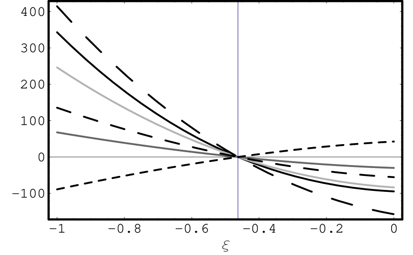
Figure 7: The run of numerators and denominators of $g_{x}^{\prime}$, $R_{1}^{\prime}$ ed $N_{1}^{\prime}$ around $\xi_{\textrm{c}}$ for $s=1$.

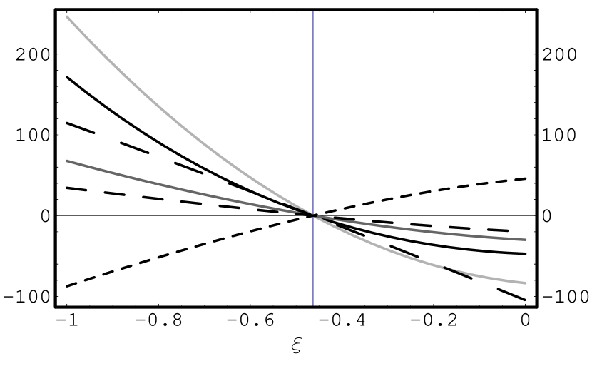
Figure 8: The run of numerators and denominators of $g_{x}^{\prime}$, $R_{1}^{\prime}$ ed $N_{1}^{\prime}$ around $\xi_{\textrm{c}}$ for $s=3$.

The dependence of all quantities upon the adimensional radius $\xi$ is shown in the figures, first for $s=3$, and then for $s=1$ ($g_{y}$ figures are obviously reported here as a result of this only section). It can easily be checked that we have indeed found two self–similar, distinct solutions, passing without divergence through the sonic point.

Figure 9: The imaginary part of $g_{y}$, when $s=3$ and $k=k_{0}$.

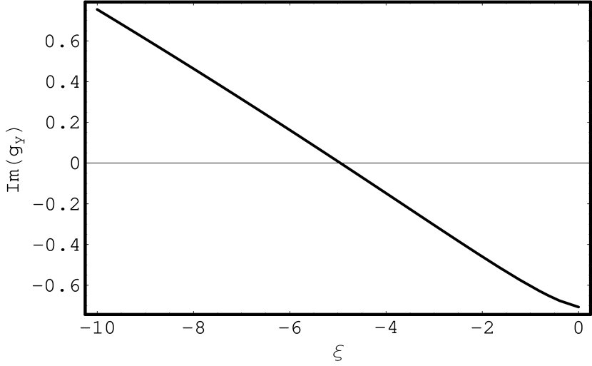
Figure 10: The imaginary part of $g_{y}$, when $s=1$ and $k=k_{0}$.

Since $s$ is real, so are $g_{x}$, $R_{1}$ and $N_{1}$. However, $g_{y}$, the only function depending on $k/k_{0}$, is purely imaginary: in fact, the boundary condition is purely imaginary and its differential equation contains only real terms multiplied by $g_{y}$ and a term containing $R_{1}$ multiplied by $i$. Furthermore, $\imath k/k_{0}$ enters $g_{y}(\xi)$ simply as a multiplicative factor. In a more intuitive way, let us consider several wrinkles of the same amplitude $\epsilon/k_{0}$, but with different wave-lengths. Clearly, the tangential component of the speed at the shock (which, after all, is the quantity that determines $g_{y}$) is proportional to $\sin\arctan\epsilon k/k_{0}$; as a wrinkle is a small perturbation, this factor reduces to $\epsilon k/k_{0}$, thus justifying previous mathematical result.