A general relativistic model of light propagation in the gravitational field of the Solar System: the dynamical case

Abstract

Modern astrometry is based on angular measurements at the micro-arcsecond level. At this accuracy a fully general relativistic treatment of the data reduction is required. This paper concludes a series of articles dedicated to the problem of relativistic light propagation, presenting the final microarcsecond version of a relativistic astrometric model which enable us to trace back the light path to its emitting source throughout the non-stationary gravity field of the moving bodies in the Solar System. The previous model is used as test-bed for numerical comparisons to the present one. Here we also test different versions of the computer code implementing the model at different levels of complexity to start exploring the best trade-off between numerical efficiency and the $\mu\textrm{as}$ accuracy needed to be reached.

1 Introduction

Modern space technology will soon provide stellar positioning with micro-arcsecond accuracy ($\mu$as). At this level one has to take into account the general relativistic effects on light propagation arising from metric perturbations due not only to the bulk mass but also to the rotational and translational motion of the bodies of the Solar System, and to their multipole structure (see Kopeikin and Mashhoon,, 2002; Klioner,, 2003; Le Poncin-Lafitte et al.,, 2004 and references therein). Our aim is to develop a Relativistic Astrometric MODel (RAMOD) which enabled us to deduce, to the accuracy of one $\mu$as, the astrometric parameters of a star in our Galaxy from observations taken by modern space-born astrometric satellites like Gaia (Turon et al.,, 2005), which are fully consistent with the precepts of General Relativity.

In this paper we present an astrometric model which contains an extension to the dynamical case, i.e. with the inclusion of the $1/c^{3}$ terms, of our previous model which was only accurate to $1/c^{2}$ (de Felice et al.,, 2004). We term it as RAMOD3 since it was intended as the successor of two previous models (de Felice et al., 1998, 2001). Following the same scheme, we shall refer to the model described here as RAMOD4.

The inclusion of terms of the order of $1/c^{3}$ corresponds to an accuracy of $0.1~{}\mu$as, at least one order of magnitude better than the expected precision of the Gaia measurements. Here we require that the Solar System is isolated and source of a weak gravitational field. These two conditions imply that the velocities of the gravitational sources within the Solar System are very small compared to the velocity of light, typically of the order of $10\,$km s^-1. Under these conditions we select a coordinate system $(x^{i},x^{0}\equiv ct)_{(i=1,\,2,\,3)}$ such that the background geometry has a post-Minkowskian form:

$$g_{\alpha\beta}=\eta_{\alpha\beta}+h_{\alpha\beta}+O\left(h^{2}\right)$$ (1)

where $\eta_{\alpha\beta}$ is the Minkowski metric and $h_{\alpha\beta}$ are small perturbations which describe effects generated by the bodies of the Solar System. These perturbations are small in the sense that $|h_{\alpha\beta}|\ll 1$, their spatial variations are of the order of $|h_{\alpha\beta}|$ while their time variations are of the order of $|h_{\alpha\beta}|/c$; here and in what follows Greek indeces run from $0$ to $3$. Clearly metric form (1) is preserved under coordinate gauge transformations of the order of $h$. The $h_{\alpha\beta}$’s contain terms of the order of at least $1/c^{2}$, hence we shall keep our approximation to first order in $h$. To the order of $1/c^{3}$ the time dependence of the background metric cannot be ignored therefore the time-like vector field $\mbox{\boldmath$\eta$\unboldmath}=\mbox{\boldmath$\partial$\unboldmath}_{0}$ tangent to the coordinate time axis, will not in general be a Killing field (namely an isometry for the space-time) unless one moves to far distances from the Solar System where the metric tends to be Minkowski’s. The components of the vector field $\eta$ are $\eta^{\mu}=\delta_{0}^{\mu},\,\eta_{\mu}=g_{0\mu}$ hence we easily deduce that the congruence $C_{\mbox{\boldmath$\eta$\unboldmath}}$, namely the family of curves having the vector field $\eta$ as tangent field, will have a non zero vorticity. From its definition

$$\omega_{\alpha\beta}=P(\eta)_{\alpha}{}^{\sigma}P(\eta)_{\beta}{}^{\rho}\nabla_{[\rho}\eta_{\sigma]},$$ (2)

where $P(\eta)_{\lambda}^{\mu}=\delta_{\lambda}^{\mu}+\eta_{\lambda}\eta^{\mu}$ is the operator which projects orthogonally to $\eta$, $\nabla_{\rho}$ the covariant $\rho-$derivative relative to the given metric and square brackets mean antisymmetrization, we have that the only non vanishing components are, to the lowest order:

$$\omega_{ij}=\partial_{[j}h_{i]0}+O\left(1/c^{4}\right),\quad i,j=1,\,2,\,3.$$ (3)

We remind that $h_{0i}$ and $\partial_{j}h_{0i}$ are $\sim O(1/c^{3})$. Condition (3) implies that the surfaces $t=\mathrm{constant}$ are not orthogonal to the integral curves of $\eta$ at least in and nearby the Solar System (de Felice et al.,, 2004). Nevertheless, because the time lines with tangent field $\eta$ are asymptotically Killing and vorticity free then the slices $S(t):\;t=\mathrm{constant}$ allow for a non ambiguous $3+1$ splitting of spacetime with a coordinate representation such that space-like coordinates are fixed within each slice. We fix the origin of the space-like coordinates at the barycenter of the Solar System and assume that the spatial coordinate axes point to distant sources chosen in such a way to assure that the system is kinematically non rotating. Adopting the IAU prescriptions (IAU,, 2000), this system is termed Barycentric Celestial Reference System (BCRS) and will be our main system since all coordinate tensorial components will be relative to it. The non stationarity of the spacetime makes the construction of a relativistic astrometric model much less straightforward than for the static case considered in de Felice et al., (2004).

In section 2 these complications are handled to define the geometrical environment for light propagation and data analysis. The spacetime metric is not diagonal since terms as $h_{0i}$ are different than zero; they are mainly generated by the velocity of the metric sources relative to the given BCRS. Then the gravitational potential at each point of the light trajectory depends on the sources in the Solar System at the appropriate retarded position as specified in section 3. This will have consequences when fixing the observables and the boundary conditions for the differential equations of the light rays in section 4. Section 5 shows how this model was numerically tested and presents the results of these tests.

In what follows we shall use geometrized units such that $c=1=G$, $G$ being the gravitational constant; with these units a mass $\mathcal{M}$, expressed in kilograms, has the dimension of a length according to the relation $M=G\mathcal{M}/c^{2}$; similarly the time coordinate $x^{0}=ct$ will be simply written as $t$ and the spatial velocities are in units of $c$. For sake of clarity, the velocity of light $c$ will appear explicitly only when we specify the order of magnitude of terms under discussion.

2 The light trajectory

We require that spacetime admits a family of hypersurfaces $S(t)$ with $t=\mathrm{constant}$ so that the spatial coordinates $\{x^{i}\}$ are fixed on each of them. As said, these surfaces are constrained by the condition of being asymptotically orthogonal to the time direction $\eta$ which will also be asymptotically Killing. In the nearby of, and of course within the Solar System, the spatial coordinates $x^{i}$ are not constant along the normals to these hypersurfaces; along them, in fact, they vary according to the shift law $\delta x^{i}\sim h_{0i}\delta t$. To the order of $1/c^{3}$, all terms proportional to $h_{0i}$ are in general not zero and cannot be made vanish in a gauge invariant way. Let us term $u$ a vector field parallel to $\eta$ and tangent to the family of timelike curves $\hat{\gamma}$, say, along which the spatial coordinates are constant; furthermore let $\hat{\sigma}$ be the parameter on these curves which makes the vector field $u$ unitary, namely $u^{\alpha}u_{\alpha}=-1$. Clearly along each integral curve of $u$ carrying the coordinates $x^{i}$, the parameter $\hat{\sigma}(x^{i},t)$ is function of the coordinate time $t$ only. By definition, the vector field $u$ has components:

$$\begin{array}[]{rcl}u^{\alpha}&=&\displaystyle{\frac{\mathrm{d}x^{\alpha}}{\mathrm{d}\hat{\sigma}}}=\mathrm{e}^{\psi}\delta_{0}^{\alpha}\\ u_{\alpha}&=&g_{0\alpha}\mathrm{e}^{\psi}\end{array}$$ (4)

where $\mathrm{e}^{\psi}=(\mathrm{d}t/\mathrm{d}\hat{\sigma})=(-g_{00})^{-1/2}$. The integral curve of $u$ through each spacetime point, identifies a local barycentric observer since, as stated, this observer is at rest in the BCRS. Consider now a null geodesic $\mit\Upsilon$ stemming from a distant star at the emission event $P_{*}:(x_{*}^{i},\,t_{*})$ and ending at the observation event $P_{0}:(x_{0}^{i},\,t_{0})$. Our aim is to find, from appropriate observational data collected at $P_{0}$, the coordinate position of the star and its proper motion. Let $k$ be the vector field tangent to $\mit\Upsilon$ and satisfying the following relations:

$$k_{\alpha}k^{\alpha} = 0$$ (5)

$$\frac{\mathrm{d}k^{\alpha}}{\mathrm{d}\lambda}+\Gamma^{\alpha}{}_{\mu\nu}k^{\mu}k^{\nu} = 0$$ (6)

where (6) is the geodesic equation, $\lambda$ is a real parameter on $\mit\Upsilon$ and $\Gamma^{\alpha}{}_{\mu\nu}$ are the connection coefficients of metric (1) given by:

$$\Gamma^{\alpha}{}_{\mu\nu}=\frac{1}{2}\eta^{\alpha\rho}\left(\partial_{\mu}h_{\rho\nu}+\partial_{\nu}h_{\rho\mu}-\partial_{\rho}h_{\mu\nu}\right)+O\left(h^{2}\right).$$ (7)

Condition (3) holds for the family of the integral curves of $u$ as well, hence $C_{\mbox{\boldmath$u$\unboldmath}}$ does not admit a global family of orthogonal hypersurfaces although such a surface always exists locally, namely in a small neighborhood of each point. This means that it is not possible to define a rest-space of the barycentric observer which covers the entire spacetime. The slice $S(t_{0})$ for example is not the rest-space of the observer $u$ at the observation point $P_{0}$. In fact, neighboring events belonging to the local rest-space of $u$ at $P_{0}$ and having spatial coordinates $x^{i}=x_{0}^{i}+\delta x^{i}$, will have a coordinate time given by

$$t=t_{0}+\mathrm{e}^{2\psi}h_{0j}\delta x^{j}.$$ (8)

The rest-space of the local barycentric observer $u$ is locally identified by the operator $P(u)^{\alpha}{}_{\beta}=\delta_{\beta}^{\alpha}+u^{\alpha}u_{\beta}$ which projects orthogonally to $u$. We define the instantaneous line of sight of $u$ as the local spatial direction of light propagation; at each point of the photon path this direction is found projecting the tangent vector k in the rest-space of $u$ namely

$$\ell^{\alpha}=P(u)^{\alpha}{}_{\beta}k^{\beta}=k^{\alpha}+u^{\alpha}(u_{\beta}k^{\beta}).$$ (9)

In this way we define a vector field $\ell$ all along the null curve $\mit\Upsilon$ (see figure 1); the knowledge of $\ell^{\alpha}$ coupled with that of $u^{\alpha}$, allows one to determine $k^{\alpha}$ and therefore to reconstruct the null trajectory followed by the photon from the star to the satellite. It is convenient to parameterize the null curve $\mit\Upsilon$ with the quantity $\sigma(\lambda)\equiv\hat{\sigma}(x(\lambda),t)$ which marks the proper time of the barycentric observer $u$ which the light trajectory crosses at each $t$.

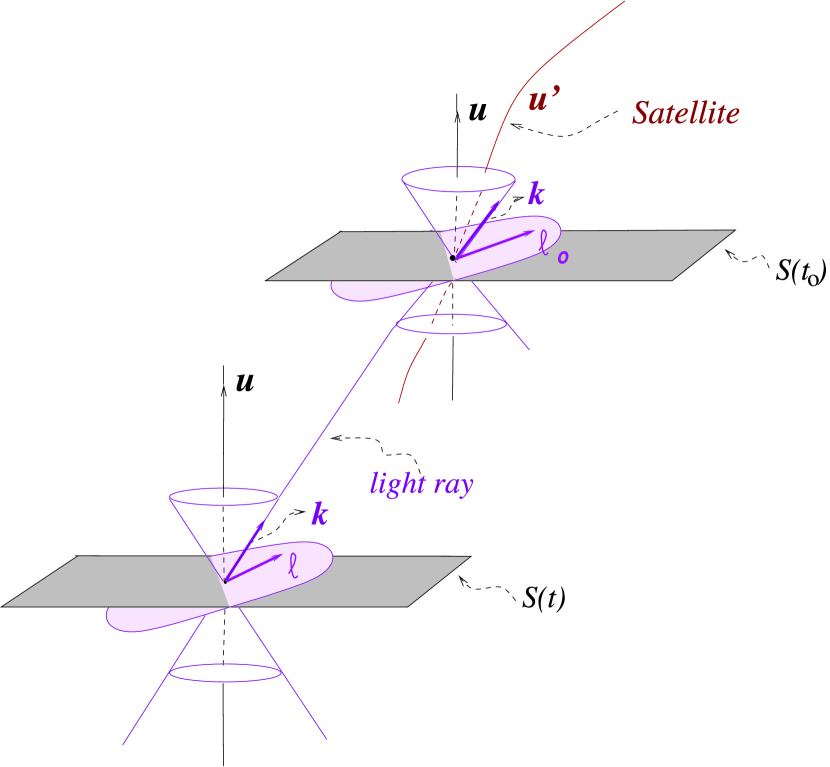
Figure 1: The light trajectory, identified by the four-vector $k$, propagates in the space-time until it is intercepted by the Gaia-like satellite at time $t_{0}$. At each point on its trajectory the light signal strikes the locally barycentric observer $u$ who identifies in its instantaneous rest-space (dotted area) the local line-of-sight $\ell$. The surfaces $S(t):t=\mathrm{const}$ do not in general coincide with the local rest-space of $u$.

If we set:

$$\bar{\ell}^{\alpha}=-\frac{\ell^{\alpha}}{u^{\rho}k_{\rho}}$$ (10)

we find from (9) that $\bar{\ell}_{\alpha}\bar{\ell}^{\alpha}=1$. If we define similarly:

$$\bar{k}^{\alpha}=-\frac{k^{\alpha}}{u^{\rho}k_{\rho}}\equiv\frac{\mathrm{d}x^{\alpha}}{\mathrm{d}\sigma}$$ (11)

then the equations which will solve the problem of finding the coordinate position of the star at the emission, are fully determined if we set along $\mit\Upsilon$

$$\bar{\ell}^{\alpha}=\frac{\mathrm{d}x^{\alpha}}{\mathrm{d}\sigma}-u^{\alpha}.$$ (12)

From (6), (7) and (10) the differential equations of the local line of sight read:

$$\frac{\mathrm{d}\bar{\ell}^{\alpha}}{\mathrm{d}\sigma} + \frac{1}{2}\left(\bar{\ell}^{0}\partial_{0}h_{00}\right)\delta_{0}^{\alpha}+\left(\bar{\ell}^{i}\partial_{i}h_{00}\right)\delta_{0}^{\alpha}+\frac{1}{2}\bar{\ell}^{\alpha}\bar{\ell}^{i}\partial_{i}h_{00}$$ (13)

$$- \left(\bar{\ell}^{\alpha}+\delta_{0}^{\alpha}\right)\left(\bar{\ell}^{i}\partial_{0}h_{0i}+\frac{1}{2}\bar{\ell}^{i}\bar{\ell}^{j}\partial_{0}h_{ij}\right)$$

$$+ \eta^{\alpha\lambda}\left[\bar{\ell}^{\beta}\bar{\ell}^{\gamma}\left(\partial_{\beta}h_{\lambda\gamma}-\frac{1}{2}\partial_{\lambda}h_{\beta\gamma}\right)+\right.$$

$$\qquad\quad\bar{\ell}^{\beta}\left(\partial_{\beta}h_{\lambda 0}+\partial_{0}h_{\lambda\beta}-\partial_{\lambda}h_{0\beta}\right)\bigg{]}$$

$$+ \eta^{\alpha\lambda}\left(\partial_{0}h_{\lambda 0}-\frac{1}{2}\partial_{\lambda}h_{00}\right)=0.$$

Let us recall an important property of the vector field $\bar{\mbox{\boldmath$\ell$\unboldmath}}$. ¿From (9) and (4), we deduce that $\bar{\ell}_{0}=P(u)_{0\beta}k^{\beta}=0$; this implies

$$\bar{\ell}^{0}=h_{0i}\bar{\ell}^{i}+O(1/c^{4}),$$ (14)

hence, to the order of $1/c^{3}$ equation (13) becomes:

$$\frac{\mathrm{d}\bar{\ell}^{\alpha}}{\mathrm{d}\sigma} + \delta_{0}^{\alpha}\bar{\ell}^{i}\partial_{i}h_{00}+\frac{1}{2}\delta_{k}^{\alpha}\bar{\ell}^{k}\bar{\ell}^{i}\partial_{i}h_{00}$$ (15)

$$- \left(\bar{\ell}^{k}\delta_{k}^{\alpha}+\delta_{0}^{\alpha}\right)\frac{1}{2}\bar{\ell}^{i}\bar{\ell}^{j}\partial_{0}h_{ij}$$

$$+ \eta^{\alpha\lambda}\left[\bar{\ell}^{i}\bar{\ell}^{j}\left(\partial_{i}h_{\lambda j}-\frac{1}{2}\partial_{\lambda}h_{ij}\right)+\right.$$

$$\qquad\quad\bar{\ell}^{i}\left(\partial_{i}h_{\lambda 0}+\partial_{0}h_{\lambda i}-\partial_{\lambda}h_{0i}\right)\bigg{]}$$

$$- \eta^{\alpha\lambda}\frac{1}{2}\partial_{\lambda}h_{00}=0$$

where $i,\,j,\,k\dots=1,\,2,\,3$. Property (14) and the requirement that our analysis is to first order in $h$ allows us to decouple the time component $\bar{\ell}^{0}$ from the spatial components $\bar{\ell}^{i}$ in the set of differential equations (15). We finally have to the $1/c^{3}$:

$$\frac{\mathrm{d}\bar{\ell}^{0}}{\mathrm{d}\sigma} - \bar{\ell}^{i}\bar{\ell}^{j}\partial_{i}h_{0j}-\frac{1}{2}\partial_{0}h_{00}=0$$ (16)

$$\frac{\mathrm{d}\bar{\ell}^{k}}{\mathrm{d}\sigma} - \frac{1}{2}\bar{\ell}^{k}\bar{\ell}^{i}\bar{\ell}^{j}\partial_{0}h_{ij}+\bar{\ell}^{i}\bar{\ell}^{j}\left(\partial_{i}h_{kj}-\frac{1}{2}\partial_{k}h_{ij}\right)$$ (17)

$$+ \frac{1}{2}\bar{\ell}^{k}\bar{\ell}^{i}\partial_{i}h_{00}+\bar{\ell}^{i}\left(\partial_{i}h_{k0}+\partial_{0}h_{ki}-\partial_{k}h_{0i}\right)$$

$$- \frac{1}{2}\partial_{k}h_{00}=0.$$

The boundary conditions needed to solve equations (12), (16) and (17) are the coordinate positions $x_{0}^{i}$ of the satellite with respect to BCRS at the observation time $t_{0}$ and the local line of sight direction $\bar{\ell}_{(0)}^{\alpha}$. While $x_{0}^{i}$ are supposed to be known, the components $\bar{\ell}_{(0)}$ need to be expressed in terms of specific observables which depend from the experimental set-up.

3 The retarded time corrections

Integration of equations (16) and (17) obviously requires that one calculates the metric coefficients $h_{\alpha\beta}$ all along the integration path. Due to the linear regime, each perturbation term can be written as:

$$h_{\alpha\beta}=\sum_{a}h_{\alpha\beta}^{(a)}$$ (18)

where the sum is extended to all bodies of the Solar System. To the selected order of $1/c^{3}$ and confining our attention to mass monopole terms of the gravitating sources, it is appropriate to consider a standard solution of Einstein’s equations in terms of retarded tensor potential (Weinberg,, 1972; Misner et al.,, 1973; de Felice and Clarke,, 1990), which can be specialized also as the Liénard-Wiechert ones (Kopeikin and Schäfer,, 1999). In the last case and in conventional units the metric coefficients read:

$$\left\{\begin{array}[]{rcl}h_{00}^{(a)}&=&\left(\displaystyle{\frac{2G\mathcal{M}^{(a)}}{c^{2}r_{{}_{\cal R}}^{(a)}}}\right)+O\left(\displaystyle{\frac{1}{c^{4}}}\right)\\[15.0pt] h_{jk}^{(a)}&=&\left(\displaystyle{\frac{2G\mathcal{M}^{(a)}}{c^{2}r_{{}_{\cal R}}^{(a)}}}\right)\delta_{jk}+O\left(\displaystyle{\frac{1}{c^{4}}}\right)\\[15.0pt] h_{0j}^{(a)}&=&\displaystyle{-\frac{2w_{j}^{(a)}}{c^{3}}}+O\left(\displaystyle{\frac{1}{c^{4}}}\right),\end{array}\right.$$ (19)

where $w_{j}$ is a spatial potential which describes the dynamical contribution to the background geometry by the relative motion of the gravitational sources and $r_{{}_{\cal R}}^{(a)}$, to be defined shortly, is the distance from the points on the photon trajectory to the barycenter of the $a$-th gravity source at the appropriate retarded time. The retarded position of the source is fixed by the intercept of its world-line with the past light-cone at any point of the photon trajectory. We shall now calculate this distance warning the reader that we shall use geometrized units ($c=1=G$) again.

Let $x^{i}(\sigma(t))$ be the spatial coordinates of a general point $P$ on the light trajectory $\mit\Upsilon$ at the coordinate time $t$ and let $x^{i}(\tilde{\sigma}(t))$ be the spatial coordinates of a general point on the spacetime trajectory of the $a$-th source, $\tilde{\sigma}$ being the parameter along that curve. The metric coefficients at the point $P$ of the light trajectory are determined by the $a$-th source of gravity when the latter was located at a point $Q$ of its trajectory at a value $\tilde{\sigma}(t^{\prime})$ of its parameter where $t^{\prime}$ is the retarded time: $t^{\prime}=t-|\mbox{\boldmath$\Delta x$\unboldmath}(t^{\prime})|$ where $|\mbox{\boldmath$\Delta x$\unboldmath}(t^{\prime})|$ is the modulus of the vector of components $\Delta x^{i}(t^{\prime})\equiv x^{i}(\sigma(t))-x^{i}(\tilde{\sigma}(t^{\prime}))$. We have dropped the suffix $(a)$. Let the world-line of the given spacetime source be described by the tangent vector:

$$\tilde{u}^{\alpha}(\tilde{\sigma})=\frac{\mathrm{d}x^{\alpha}}{\mathrm{d}\tilde{\sigma}}=-(u_{\beta}\tilde{u}^{\beta})\left(u^{\alpha}+\tilde{v}^{\alpha}\right),$$ (20)

where $\tilde{v}^{\alpha}$ is the $\alpha$-component of the physical spatial velocity of the source in the rest frame of the local barycentric observer $u$ whose components $u^{\alpha}$ are given by (4); hence we have:

$$\frac{\mathrm{d}x^{i}}{\mathrm{d}\tilde{\sigma}}=-(u_{\beta}\tilde{u}^{\beta})\tilde{v}^{i}\qquad(i=1,\,2,\,3).$$ (21)

The distance $r_{{}_{\cal R}}$ at the retarded time $t^{\prime}$ along the world-line of the source is given by $r_{{}_{\cal R}}=-\tilde{u}_{\beta}\Delta x^{\beta}$ (see e.g. Kopeikin and Schäfer,, 1999). Since we require that our model is accurate to the order of $1/c^{3}$ then, recalling that the metric potentials are at least $1/c^{2}$, it suffices that the retarded distance $r_{{}_{\cal R}}$ is determined only up to $(1/c)$. From (20) and recalling that $\Delta x^{i}(t^{\prime})$ is taken along the generators of a light-cone, we have

$$r_{{}_{\cal R}}=|\mbox{\boldmath$\Delta x$\unboldmath}(t^{\prime})|-\delta_{ij}\tilde{v}^{i}(t^{\prime})\Delta x^{j}(t^{\prime}).$$ (22)

Before proceeding, let us briefly recall the concept of spatial distance. Let $r$, say, be such a distance from $P$ to the $a$-th source at $Q$ as it would be measured by the barycentric observer $u$ in $P$. From the very definition of a spatial distance, the quantity $r$ is the separation between the events $P$ and $\hat{Q}$ the latter being the event of the history of the observer $u$ going trough $Q$ which is simultaneous to $P$ with respect to $u$ in $P$ (see figure 2).

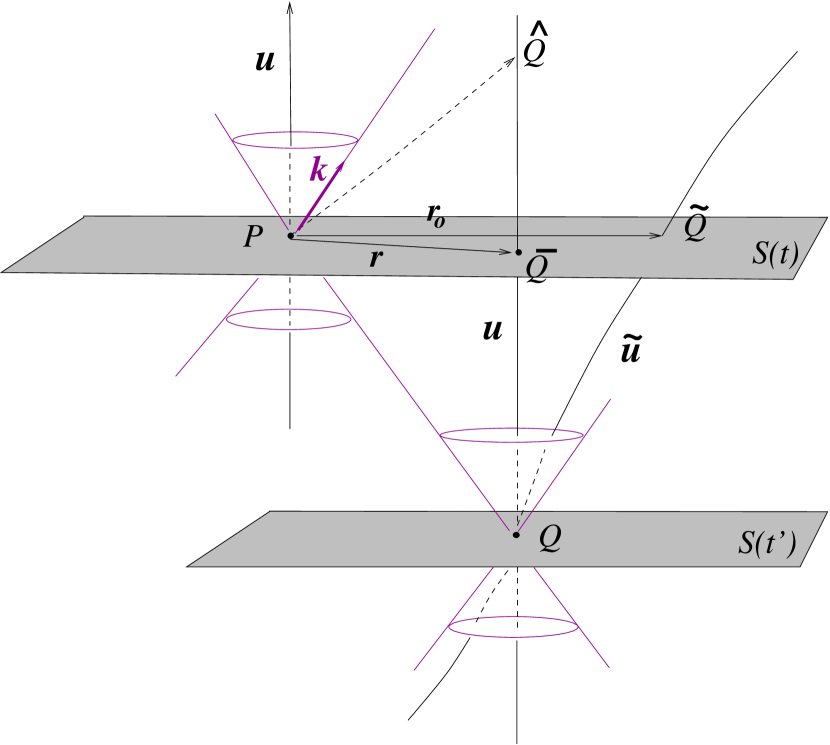
Figure 2: The metric coefficients in $P$ at time $t$ are determined by the gravity source located in $Q$ at the retarded time $t^{\prime}$. At time $t$ the gravity source will be in $\tilde{Q}$ but the distance $r$ which enters the metric coefficients is that between the events $P$ and $\hat{Q}$; the latter has the same spatial coordinates of $Q$ and $\bar{Q}$ but is simultaneous to $P$ with respect to the locally barycentric observer $u$ in $P$. Here we confuse $\hat{Q}$ with $\bar{Q}$ the error being of the order of $1/c^{4}$. In the figure the suffix $(a)$ of the bodies are dropped. $\tilde{Q}$ is the position on $S(t)$ of the planet which is moving along its world line.

From the condition of simultaneity, the coordinates of $\hat{Q}$ are given by:

$$x^{i}_{{}_{\hat{Q}}} = x^{i}(\tilde{\sigma}(t^{\prime}))$$

$$t_{{}_{\hat{Q}}} = t+\int^{x^{i}(\sigma(t))}_{x^{i}(\tilde{\sigma}(t^{\prime}))}\mathrm{e}^{2\psi}h_{0j}(x^{\prime})\,\mathrm{d}x^{{}^{\prime}j}.$$

Here the integral is at least of the order of $1/c^{3}$ and since it would enter terms of an order higher than that we can neglect it and confuse $\hat{Q}$ with the event $\bar{Q}$ which is the intersection of the world-line of $u$ through $Q$ with the surface $S(t)$. To first order in $h$ and terming $\tau$ the parameter along the shortest space-like path (geodesic) connecting $P$ to $\bar{Q}$ on $S(t)$, the required spatial distance reads:

$$r = \int^{\tau(P)}_{\tau(\bar{Q})}\sqrt{{P(u)_{\alpha\beta}\xi^{\alpha}\xi^{\beta}}}\,\mathrm{d}\tau$$ (23)

$$= \int^{\tau(P)}_{\tau(\bar{Q})}\sqrt{{(\delta_{ij}+h_{ij})\xi^{i}\xi^{j}}}\,\mathrm{d}\tau+O(h^{2})$$

where $\xi^{\alpha}\equiv\mathrm{d}x^{\alpha}/\mathrm{d}\tau$ is the unitary space-like tangent to the line of integration. Notice that the integral in (23) contains terms of the order $[1/c^{0}+O(1/c^{2})]$ hence, on the basis of what we said before, we can retain only the Euclidean part, namely:

$$r = \int^{\tau(P)}_{\tau(\bar{Q})}\sqrt{{\delta_{ij}\xi^{i}\xi^{j}}}\,\mathrm{d}\tau+O(1/c^{2})$$ (24)

$$= \sqrt{\delta_{ij}[x^{i}(\sigma(t))-x^{i}(\tilde{\sigma}(t^{\prime}))][x^{j}(\sigma(t))-x^{j}(\tilde{\sigma}(t^{\prime}))]}+O(1/c^{2})$$

$$\equiv |\mbox{\boldmath$\Delta x$\unboldmath}(t^{\prime})|+O(1/c^{2}).$$

Here we have made the identifications:

$$x^{i}(\tau(\bar{Q})) = x^{i}(\tilde{\sigma}(t^{\prime}))$$

$$x^{i}(\tau(P)) = x^{i}(\sigma(t)).$$

From (24) and (22) we can write the metric coefficients (19) as

$$\left\{\begin{array}[]{rcl}h_{00}^{(a)}&=&\left(\displaystyle{\frac{2G\mathcal{M}^{(a)}}{c^{2}r^{(a)}}}\right)\left(1+\mathbf{v}^{(a)}\cdot\hat{\mathbf{n}}^{(a)}\right)+O\left(\displaystyle{\frac{1}{c^{4}}}\right)\\[15.0pt] h_{jk}^{(a)}&=&\left(\displaystyle{\frac{2G\mathcal{M}^{(a)}}{c^{2}r^{(a)}}}\right)\left(1+\mathbf{v}^{(a)}\cdot\hat{\mathbf{n}}^{(a)}\right)\delta_{jk}+O\left(\displaystyle{\frac{1}{c^{4}}}\right)\\[15.0pt] h_{0j}^{(a)}&=&\displaystyle{-\frac{2w_{j}^{(a)}}{c^{3}}}+O\left(\displaystyle{\frac{1}{c^{4}}}\right),\end{array}\right.$$ (25)

where $\mathbf{n}^{(a)}=\mathbf{r}^{(a)}/r^{(a)}$, all quantities here being calculated at the retarded time $t^{\prime}$. Having defined as retarded distance the quantity $r_{\cal R}$, we shall term reduced distance the quantity $r$ as in (24).

It is convenient, for computational purposes, to express the distance $r$ in terms of quantities defined all at the same time $t$ of metric determination. To this purpose few more steps are needed for the correct identification of the retarded time corrections. Integrating (21) from $\tilde{\sigma}(t^{\prime})$ to $\tilde{\sigma}(t)$ which correspond respectively to the points $Q$ and $\tilde{Q}$ as shown in figure 2

$$x^{i}(\tilde{\sigma}(t^{\prime}))=x^{i}(\tilde{\sigma}(t))+\int^{\tilde{\sigma}(t)}_{\tilde{\sigma}(t^{\prime})}(u_{\beta}\tilde{u}^{\beta})\tilde{v}^{i}(\tilde{\sigma})\,\mathrm{d}\tilde{\sigma}\cdots$$ (26)

the integral being taken along the world-line of the gravity source. From this it follows:

$$x^{i}(\sigma(t))-x^{i}(\tilde{\sigma}(t^{\prime}))=x^{i}(\sigma(t))-x^{i}(\tilde{\sigma}(t))-\int^{\tilde{\sigma}(t)}_{\tilde{\sigma}(t^{\prime})}(u_{\beta}\tilde{u}^{\beta})\tilde{v}^{i}(\tilde{\sigma})\,\mathrm{d}\tilde{\sigma}+\cdots.$$ (27)

Notice that $x^{i}(\tilde{\sigma}(t))$ are the spatial coordinates of the gravity source at the time $t$ in the BCRS; these are supposed to be known; also the components of its spatial velocity $\tilde{v}^{i}(\tilde{\sigma}(t))$ with respect to the local barycentric observer at time $t$ are assumed to be known. From (23) and (27) we then have:

$$r= \left\{\vphantom{\displaystyle{\int^{\tilde{\sigma}(t)}_{\tilde{\sigma}(t^{\prime})}}}\delta_{ij}\right. \left[x^{i}(\sigma(t))-x^{i}(\tilde{\sigma}(t))-\int^{\tilde{\sigma}(t)}_{\tilde{\sigma}(t^{\prime})}(u_{\beta}\tilde{u}^{\beta})\tilde{v}^{i}(\tilde{\sigma})\,\mathrm{d}\tilde{\sigma}\cdots\right]\times$$ (28)

$$\left.\left[x^{j}(\sigma(t))-x^{j}(\tilde{\sigma}(t))-\int^{\tilde{\sigma}(t)}_{\tilde{\sigma}(t^{\prime})}(u_{\beta}\tilde{u}^{\beta})\tilde{v}^{j}(\tilde{\sigma})\,\mathrm{d}\tilde{\sigma}+\cdots\right]\right\}^{1/2}+O\left(\frac{1}{{c^{2}}}\right)$$

Setting

$$\Delta x^{i}(t)=x^{i}(\sigma(t))-x^{i}(\tilde{\sigma}(t)).$$ (29)

and recalling that

$$-(u^{\alpha}\tilde{u}_{\alpha})=(1-\tilde{v}^{2})^{-1/2}$$ (30)

$\tilde{v}$ being the (modulus of the) spatial velocity of the gravity source with respect to the local barycentric observer, equation (28) writes as:

$$r= \left\{\vphantom{\displaystyle{\int^{\tilde{\sigma}(t)}_{\tilde{\sigma}(t^{\prime})}}}\delta_{ij}\right. \left[\Delta x^{i}(t)+\int^{\tilde{\sigma}(t)}_{\tilde{\sigma}(t^{\prime})}\left(1+\frac{1}{2}\tilde{v}^{2}\right)\tilde{v}^{i}(\tilde{\sigma})\,\mathrm{d}\tilde{\sigma}\cdots\right]\times$$ (31)

$$\left.\left[\Delta x^{j}(t)+\int^{\tilde{\sigma}(t)}_{\tilde{\sigma}(t^{\prime})}\left(1+\frac{1}{2}\tilde{v}^{2}\right)\tilde{v}^{j}(\tilde{\sigma})\,\mathrm{d}\tilde{\sigma}+\cdots\right]\right\}^{1/2}$$

which can be written as follows:

$$r=\left[r_{0}^{2}+2\delta_{ij}\Delta x^{i}(t)\int^{\tilde{\sigma}(t)}_{\tilde{\sigma}(t^{\prime})}\tilde{v}^{j}\,\mathrm{d}\tilde{\sigma}+\delta_{ij}\int^{\tilde{\sigma}(t)}_{\tilde{\sigma}(t^{\prime})}\tilde{v}^{i}\,\mathrm{d}\tilde{\sigma}\int^{\tilde{\sigma}(t)}_{\tilde{\sigma}(t^{\prime})}\tilde{v}^{j}\,\mathrm{d}\tilde{\sigma}\right]^{1/2}+O\left(\frac{1}{{c^{2}}}\right)$$ (32)

where at any $t$

$$r_{0}=\sqrt{\delta_{ij}\Delta x^{i}(t)\Delta x^{j}(t)}.$$ (33)

For the bodies of the Solar System the quantities $\int^{\tilde{\sigma}(t)}_{\tilde{\sigma}(t^{\prime})}\tilde{v}^{j}(\tilde{\sigma})\,\mathrm{d}\tilde{\sigma}$ are always much smaller then $r_{0}$; even in the extreme case of a light ray skimming the surface of a planet the integral goes to zero while $r_{0}$ remains of the order of the body’s radius. Thus the following Taylor expansion is justified. Remembering that $(1+x)^{1/2}\approx 1+(1/2)x-(1/8)x^{2}+\cdots$, then to the given order we have from equation (32):

$$r = r_{0}\left\{\vphantom{\left[\int_{\tilde{\sigma}(t^{\prime})}^{\tilde{\sigma}(t)}\right]^{2}}1+\frac{1}{r_{0}^{2}}\left[\delta_{ij}\Delta x^{i}(t)\int_{\tilde{\sigma}(t^{\prime})}^{\tilde{\sigma}(t)}\tilde{v}^{j}(\tilde{\sigma})\,\mathrm{d}\tilde{\sigma}+\frac{1}{2}\delta_{ij}\int_{\tilde{\sigma}(t^{\prime})}^{\tilde{\sigma}(t)}\tilde{v}^{i}(\tilde{\sigma})\,\mathrm{d}\tilde{\sigma}\int_{\tilde{\sigma}(t^{\prime})}^{\tilde{\sigma}(t)}\tilde{v}^{j}(\tilde{\sigma})\,\mathrm{d}\tilde{\sigma}\right]\right.$$ (34)

$$- \left.\frac{1}{8r_{0}^{4}}\left[\delta_{ij}\Delta x^{i}(t)\int_{\tilde{\sigma}(t^{\prime})}^{\tilde{\sigma}(t)}\tilde{v}^{j}(\tilde{\sigma})\,\mathrm{d}\tilde{\sigma}+\frac{1}{2}\delta_{ij}\int_{\tilde{\sigma}(t^{\prime})}^{\tilde{\sigma}(t)}\tilde{v}^{i}(\tilde{\sigma})\,\mathrm{d}\tilde{\sigma}\int_{\tilde{\sigma}(t^{\prime})}^{\tilde{\sigma}(t)}\tilde{v}^{j}(\tilde{\sigma})\,\mathrm{d}\tilde{\sigma}\right]^{2}\right\}$$

$$+ O\left(\frac{1}{c^{2}}\right).$$

Evidently, the $1/c^{2}$ contribution of the relative velocity of the gravitating sources to the retarded time correction can be neglected. The integrations in (34) contain the unknown $r$ implicitly in $\tilde{\sigma}(t^{\prime})$ and this makes the calculations rather cumbersome, however order of magnitude considerations allow one to identify the proper-time $\tilde{\sigma}(t)$ with the coordinate time $t$ so achieving a considerable simplification. From (20), in fact, we have

$$\tilde{u}^{0}=\frac{\mathrm{d}t}{\mathrm{d}\tilde{\sigma}}=\tilde{\gamma}\left(u^{0}+\tilde{v}^{0}\right)$$ (35)

where $\tilde{\gamma}=-\tilde{u}_{\sigma}u^{\sigma}=(1-\tilde{v}^{2})^{-1/2}$ is the Lorentz factor of the gravity source relative to the local barycentric observer. Recalling (1) and (4) we easily get:

$$u^{0} = 1+\frac{1}{2}h_{00}+O\left(\frac{1}{c^{4}}\right)$$

$$\tilde{v}^{0} = O\left(\frac{1}{c^{4}}\right)$$ (36)

the latter relation arising from the condition $\tilde{v}_{\alpha}u^{\alpha}=0$. Thus equation (35) becomes:

$$\frac{\mathrm{d}t}{\mathrm{d}\tilde{\sigma}}=1+\frac{1}{2}h_{00}+\frac{1}{2}\tilde{v}^{2}+O\left(\frac{1}{c^{4}}\right)$$ (37)

which leads to

$$\mathrm{d}\tilde{\sigma}=\mathrm{d}t+O\left(\frac{1}{c^{2}}\right).$$ (38)

A similar argument applies to the integration variable $\sigma$ entering the master equations (16) and (17) and so, to the required order, we can calculate the individual terms in (16) and (17) and in (34) confusing the barycentric and the gravity source proper-times with the coordinate time $t$. From the above considerations and setting $\Delta\tilde{x}^{i}(t,t^{\prime})\equiv\tilde{x}^{i}(t)-\tilde{x}^{i}(t^{\prime})=\int_{t^{\prime}}^{t}\tilde{v}^{i}(t)\,\mathrm{d}t+O(1/c^{2})$ with $\tilde{x}^{i}(t)\equiv x^{i}(\tilde{\sigma}(t))$, equation (34) becomes:

$$r = r_{0}\left\{\vphantom{\left[\frac{1}{2}\right]^{2}}1+\frac{1}{r_{0}^{2}}\left[\delta_{ij}\Delta x^{i}(t)\Delta\tilde{x}^{j}(t,t^{\prime})+\frac{1}{2}\delta_{ij}\Delta\tilde{x}^{i}(t,t^{\prime})\Delta\tilde{x}^{j}(t,t^{\prime})\right]\right.$$ (39)

$$- \left.\frac{1}{8r_{0}^{4}}\left[\delta_{ij}\Delta x^{i}(t)\Delta\tilde{x}^{j}(t,t^{\prime})+\frac{1}{2}\delta_{ij}\Delta\tilde{x}^{i}(t,t^{\prime})\Delta\tilde{x}^{j}(t,t^{\prime})\right]^{2}\right\}+O\left(\frac{1}{c^{2}}\right).$$

It is clear that, being $\tilde{v}^{j}(t)$ a bounded function, the integrals in (39) remain finite when $r_{0}\rightarrow\infty$, hence in that limit we have that $r\rightarrow r_{0}$ as expected. Let us now define $\mathbf{r}_{0}=\{\Delta x^{i}(t)\}$ and $\tilde{\mathbf{r}}=\{\Delta\tilde{x}^{i}(t,t^{\prime})\}$ with $i=1,\,2,\,3$; since the orbits of the spacetime sources are bounded then $\tilde{\mathbf{r}}$ is finite while $\mathbf{r}_{0}$ can grow to infinity, then we retain only terms of the order of $(\tilde{\mathbf{r}}/\mathbf{r}_{0})^{2}$. Equation (39) can then be cast in vectorial form:

$$r=r_{0}\left[1+\frac{1}{r_{0}^{2}}\left(\mathbf{r}_{0}\cdot\tilde{\mathbf{r}}+\frac{1}{2}\tilde{\mathbf{r}}\cdot\tilde{\mathbf{r}}\right)-\frac{1}{8r_{0}^{4}}\left(\mathbf{r}_{0}\cdot\tilde{\mathbf{r}}\right)^{2}+O\left(\left(\frac{||\tilde{\mathbf{r}}||}{||\mathbf{r}_{0}||}\right)^{3}\right)\right]+O\left(\frac{1}{c^{2}}\right).$$ (40)

It should be stressed here that (40) is an implicit equation since $\tilde{\mathbf{r}}$ is function of $r$ in its turn.

4 The boundary conditions

The differential equations (16) and (17) are of the general form:

$$\frac{\mathrm{d}\bar{\ell}^{\alpha}}{\mathrm{d}\sigma}=\mathcal{F}^{\alpha}(\partial_{\beta}h(x,y,z,t),\bar{\ell}^{i}(\sigma(x)))$$ (41)

where $\mathcal{F}^{\alpha}$ are real, non singular, smooth functions of their arguments. A general solution of (41) is

$$\bar{\ell}^{\alpha}=\bar{\ell}^{\alpha}(\sigma,\bar{\ell}_{(0)}^{k})$$ (42)

where $\bar{\ell}_{(0)}^{k}$ are the components of the vector $\bar{\mbox{\boldmath$\ell$\unboldmath}}$ at the observation and represent the boundary values that we need to fix in order to integrate (41). These boundary conditions can only be expressed in terms of the satellite observations. In the case of Gaia the observables are the angles that the incoming light ray forms with the spatial axes of the satellite attitude triad. The latter is a set of three orthonormal space-like vectors which are comoving with the satellite and define its rest frame; their coordinate components are denoted as $\{E_{\hat{a}}^{\alpha}\}_{\hat{a}=1,2,3}$ and satisfy the condition $E_{\hat{a}}^{\alpha}E_{\alpha\hat{b}}=\delta_{\hat{a}\hat{b}}$. The observables are given by:

$$\cos\psi_{(E_{\hat{a}},\bar{\ell})}\equiv\mathbf{e}_{\hat{a}}=\frac{P(u^{\prime})_{\alpha\beta}k^{\alpha}E_{\hat{a}}^{\beta}}{(P(u^{\prime})_{\alpha\beta}k^{\alpha}k^{\beta})^{1/2}};$$ (43)

$P(u^{\prime})_{\alpha\beta}$ is the operator which projects into the satellite’s rest-frame, namely:

$$P(u^{\prime})_{\alpha\beta}=g_{\alpha\beta}+u^{\prime}_{\alpha}u^{\prime}_{\beta}$$ (44)

and $\mbox{\boldmath$u$\unboldmath}^{\prime}$ is the time-like and unitary satellite four velocity. The latter is given by

$$\mbox{\boldmath$u$\unboldmath}^{\prime}=T_{s}(\mbox{\boldmath$\partial$\unboldmath}_{t}+\beta_{1}\mbox{\boldmath$\partial$\unboldmath}_{x}+\beta_{2}\mbox{\boldmath$\partial$\unboldmath}_{y}+\beta_{3}\mbox{\boldmath$\partial$\unboldmath}_{z}),$$ (45)

where $\mbox{\boldmath$\partial$\unboldmath}_{\alpha}$’s are the coordinate basis vectors relative to the barycentric celestial reference system, $\beta_{i}$ are the coordinate components of the satellite three-velocity with respect to the barycenter of the Solar System. Here the subscripts refer to contravariant components not to confuse them with power indeces. It is important to stress that the modulus of $\beta_{i}$ is not the physical velocity of the satellite with respect to the local barycentric observer $u$, nor the $\beta_{i}$ are its physical components. The physical velocity instead, namely the quantity which would be measured, is given by the modulus of the four vector with components:

$$\nu^{\alpha}=\frac{1}{\gamma}\left(u^{\prime\alpha}-\gamma u^{\alpha}\right)$$ (46)

where $\gamma$ is the instantaneous satellite’s Lorentz factor. Form (46) it follows:

$$\nu^{0} = -\frac{1}{2}U\beta^{2}=O(1/c^{4})$$

$$\nu^{i} = (1+U)\beta_{i}+O(1/c^{4})$$ (47)

where $2U=h_{00}$ $\beta^{2}=\beta_{1}^{2}+\beta_{2}^{2}+\beta_{3}^{2}$; hence $\nu^{i}$ coincides with $\beta_{i}$ only to the order of $1/c^{2}$. Finally we recall that $u^{\prime\alpha}u^{\prime}_{\alpha}=-1$ and this relation fixes the time factor of $\mbox{\boldmath$u$\unboldmath}^{\prime}$ as $T_{s}=1+\frac{1}{2}(h_{00}+\beta^{2})$. From (12) and (45), equation (43) can be written more explicitely as:

$$\cos\psi_{(E_{\hat{a}},\bar{\ell})}\equiv\mathbf{e}_{\hat{a}}=\frac{P(u^{\prime})_{\alpha\beta}(\bar{\ell}_{(0)}^{\alpha}+u^{\alpha}){E_{\hat{a}}}^{\beta}}{[u^{\prime}_{\rho}(\bar{\ell}_{(0)}^{\rho}+u^{\rho})]^{1/2}}=-\frac{(\bar{\ell}_{(0)}^{\beta}-\nu^{\beta})E_{\hat{a}\beta}}{\gamma\nu_{\alpha}\bar{\ell}_{(0)}^{\alpha}-\gamma}$$ (48)

all terms being calculated at the observation time. We easily see that all quantities contained in (48) are known except $\bar{\ell}_{(0)}^{i}$ which obviously are the unknown boundary conditions, as stated. In order to deduce them correctly one needs the components of the satellite attitude triad. They have been deduced in explicit form in Bini et al., (2003) (see equations (4.17) and Appendix B of that paper). Here we shall cast them in a form easier to handle in direct calculations.

The satellite is expected to rotate with an angular velocity $\omega_{r}$ about an axis (its $\hat{x}$-axis) which forms an angle $\alpha$ with respect to the instantaneous local direction to the Sun. The spin axis then precesses about the direction to the Sun with an angular velocity $\omega_{p}$. The attitude triad will then depend on this parameter specification as follows (Bini et al.,, 2003):

$$E_{\hat{1}}^{\alpha} = \cos\alpha{\lambda_{\hat{1}}^{\alpha}}{}{{}_{(\mathrm{bs})}}-\sin\alpha\cos(\omega_{p}t){\lambda_{\hat{2}}^{\alpha}}{}{{}_{(\mathrm{bs})}}-\sin\alpha\cos(\omega_{p}t){\lambda_{\hat{3}}^{\alpha}}{}{{}_{(\mathrm{bs})}}$$ (49)

$$E_{\hat{2}}^{\alpha} = -\sin\alpha\sin(\omega_{r}t){\lambda_{\hat{1}}^{\alpha}}{}{{}_{(\mathrm{bs})}}+$$

$$+[\cos(\omega_{r}t)\cos(\omega_{p}t)-\sin(\omega_{r}t)\sin(\omega_{p}t)\cos\alpha]{\lambda_{\hat{2}}^{\alpha}}{}{{}_{(\mathrm{bs})}}$$

$$+[\cos(\omega_{r}t)\sin(\omega_{p}t)+\sin(\omega_{r}t)\cos(\omega_{p}t)\cos\alpha]{\lambda_{\hat{3}}^{\alpha}}{}{{}_{(\mathrm{bs})}}$$

$$E_{\hat{3}}^{\alpha} = -\sin\alpha\cos(\omega_{r}t){\lambda_{\hat{1}}^{\alpha}}{}{{}_{(\mathrm{bs})}}$$

$$-[\sin(\omega_{r}t)\cos(\omega_{p}t)+\cos(\omega_{r}t)\sin(\omega_{p}t)\cos\alpha]{\lambda_{\hat{2}}^{\alpha}}{}{{}_{(\mathrm{bs})}}$$

$$+[-\sin(\omega_{r}t)\sin(\omega_{p}t)+\cos(\omega_{r}t)\cos(\omega_{p}t)\cos\alpha]{\lambda_{\hat{3}}^{\alpha}}{}{{}_{(\mathrm{bs})}}$$

where $\alpha$ takes values as ($t,\,x,\,y,\,z$) and $\{{\mbox{\boldmath$\lambda$\unboldmath}_{\hat{a}}}{}{{}_{(\mathrm{bs})}}\}$ is the Lorentz boosted triad adapted to the satellite whose components are given in explicit form in the appendix A.

4.1 The spatial velocity of the Gaia satellite

To make the boundary conditions complete we need an operational definition of the satellite’s spatial physical velocity $\nu^{i}$. The satellite trajectory will be close to that of the outer Lagrangian point $L_{2}$ relative to the Earth-Sun system. The world lines of $L_{2}$ and Gaia never intersect because Gaia moves around $L_{2}$ in a halo type orbit. Hence to define Gaia’s spatial velocity with respect to $L_{2}$ we have first to fix a coordinate frame comoving with $L_{2}$. Denoting the coordinates with respect to $L_{2}$ with a bar, we define:

$$\bar{t}=t\qquad\bar{x}_{{}_{G}}=x_{{}_{G}}-x_{{}_{L_{2}}}$$

hence the four-velocity of Gaia in the coordinate frame of $L_{2}$ reads:

$$\bar{u}_{{}_{G}}^{\alpha}=\bar{u}_{{}_{G}}^{0}\left(\delta_{0}^{\alpha}+\bar{\beta}_{{}_{G}}^{i}\delta_{i}^{\alpha}\right)$$

where

$$\bar{\beta}_{{}_{G}}^{i}=\frac{\mathrm{d}\bar{x}_{{}_{G}}^{i}}{\mathrm{d}t}$$

are the coordinate components of Gaia’s spatial velocity with respect to $L_{2}$.

Let us identify what are the unknowns and what is known. Our task is to express the formers in terms of the latters. The unknowns are the components of the spatial velocity of Gaia with respect to the local barycentric observer, namely $\nu^{i}$. The known quantities are: (i) the components of the coordinate spatial velocity of $L_{2}$ with respect to the local barycentric observer namely $\beta_{L_{2}}^{i}=\mathrm{d}x_{L_{2}}^{i}/\mathrm{d}t$; (ii) the components of the spatial velocity of Gaia with respect to $L_{2}$, namely $\bar{\beta}_{G}$; (iii) the metric coefficients at the position of Gaia.

Let us express $\nu^{i}$ in terms of the known quantities. From (46) it follows that

$$\nu^{i}=\beta^{i}\left(1+\frac{1}{2}h_{00}+O(1/c^{4})\right)$$ (52)

hence, recalling that $\beta^{i}=\mathrm{d}x_{G}^{i}/\mathrm{d}t$, we have

$$\beta^{i}=\frac{\mathrm{d}\bar{x}_{G}^{i}}{\mathrm{d}t}+\frac{\mathrm{d}x_{L_{2}}^{i}}{\mathrm{d}t}=\bar{\beta}_{G}^{i}+\beta_{L_{2}}^{i}$$ (53)

namely

$$\nu^{i}=\bar{\beta}_{G}^{i}\left(1+\frac{1}{2}h_{00}+O(1/c^{4})\right)+\nu_{L_{2}}^{i}.$$ (54)

In (52) and (54) the gravitational potential $h_{00}$ is calculated at the position of the satellite.

5 Testing RAMOD4

The most efficient way to test RAMOD4 is to compare the results of the integration of its equations of motion with those of RAMOD3. We expect that the differences between the two models are of the order of $5\cdot 10^{-11}$ rad i.e. $\sim 10\mu$as (see section 7 of de Felice et al.,, 2004). Obviously the practical implementation of these equations requires the precise specification of some of its ingredients. First of all an explicit form of the metric (25) should be chosen; in this context and to the prescribed order of $1/c^{3}$ we chose, as stated early, a solution of Einstein’s equations based on the Liénard-Wiechert tensor potentials in terms of which, we recall, the post-Minkowskian metric perurbations take the form

$$h_{00} = \sum_{a}\frac{2G\mathcal{M}^{(a)}}{c^{2}r^{(a)}}\left(1+\mathbf{v}^{(a)}\cdot\hat{\mathbf{n}}^{(a)}\right)+O\left(\frac{1}{c^{4}}\right)$$

$$h_{0i} = \sum_{a}-\frac{4G\mathcal{M}^{(a)}}{c^{3}r^{(a)}}\tilde{v}_{i}^{(a)}=-2h_{00}\frac{\tilde{v}_{i}}{c}+O\left(\frac{1}{c^{4}}\right)$$ (55)

$$h_{ij} = \sum_{a}\frac{2G\mathcal{M}^{(a)}}{c^{2}r^{(a)}}\left(1+\mathbf{v}^{(a)}\cdot\hat{\mathbf{n}}^{(a)}\right)\delta_{ij}=h_{00}\delta_{ij}+O\left(\frac{1}{c^{4}}\right).$$

where the potential $w_{j}^{(a)}$ due to the relative velocities of the bodies is equal to

$$w_{j}^{(a)}=-\frac{4G\mathcal{M}^{(a)}}{c^{3}r^{(a)}}\tilde{v}_{j}^{(a)}+O\left(\frac{1}{c^{4}}\right).$$

The coordinate form for the master equations obtained by using the explicit metric components (55) in (17) is reported in appendix B. The reduced distance $r^{(a)}$ which enters equations (55) will be treated separately in subsection 5.1.

The boundary conditions which are needed to integrate (17) can be specified only after the tetrad describing the motion of the observer is given explicitely. Our goal is to compare this new model with RAMOD3, hence a natural choice is a tetrad that makes the measurements compatible with those described in de Felice et al., (2004), that is, a phase-locked tetrad associated to an observer moving on a circular orbit around the barycenter of the Solar System on the plane $z=0$.

The four-velocity $u^{\prime\alpha}$ of this observer writes

$$u^{\prime\alpha}=\mathrm{e}^{\psi^{\prime}}\left[\delta_{0}^{\alpha}-\omega\left(y_{\mathrm{s}}-y_{\odot}\right)\delta_{x}^{\alpha}+\omega\left(x_{\mathrm{s}}-x_{\odot}\right)\delta_{y}^{\alpha}\right],$$ (56)

where $\omega$ is the angular velocity of the observer, $x_{\odot}$ and $y_{\odot}$ are the barycentric position of the Sun, and $\mathrm{e}^{\psi^{\prime}}$ is a normalization factor required by the condition $u^{\prime\alpha}u^{\prime}_{\alpha}=-1$. Since in RAMOD4 the only non-vanishing terms of the metric are $g_{|\alpha|\alpha}$ and $g_{0i}$, this factor is

$$\mathrm{e}^{\psi^{\prime}}=\left\{-\left[g_{00}-2\omega\left(y_{\mathrm{s}}-y_{\odot}\right)g_{0x}+2\omega\left(x_{\mathrm{s}}-x_{\odot}\right)g_{0y}+\omega^{2}\left(y_{\mathrm{s}}-y_{\odot}\right)^{2}g_{xx}+\omega^{2}\left(x_{\mathrm{s}}-x_{\odot}\right)^{2}g_{yy}\right]\right\}^{-1/2}.$$

The explicit expression of the components of the tetrad spatial axes can be deduced by the components of the tetrad $\left\{{\lambda_{\hat{a}}}{}{{}_{(\mathrm{bs})}}\right\}$ given in eqs.(A3-A19) setting $\theta=0$ and substituting the velocity components of the observer with the following expressions

$$\begin{array}[]{rcl}\beta_{1}&=&-\omega\left(y_{\mathrm{s}}-y_{\odot}\right)\mathrm{e}^{\psi^{\prime}}\\ \beta_{2}&=&\omega\left(x_{\mathrm{s}}-x_{\odot}\right)\mathrm{e}^{\psi^{\prime}}\\ \beta_{3}&=&0\end{array}$$ (57)

which describe, as stated, a spatially circular orbit.

From (57) and following the conventions in Bini et al., (2003), the tetrad component ${\lambda}{}{{}_{(\mathrm{bs})}}_{\hat{1}}^{0}$ become

$$\begin{array}[]{rcl}{\lambda_{\hat{1}}^{0}}{}{{}_{(\mathrm{bs})}}&=&\left(\frac{3}{2}h_{00}+\frac{1}{2}\omega^{2}R^{2}\mathrm{e}^{2\psi^{\prime}}+1\right)\left[-\omega\left(y_{\mathrm{s}}-y_{\odot}\right)\mathrm{e}^{\psi^{\prime}}\cos\phi_{\mathrm{s}}+\omega\left(x_{\mathrm{s}}-x_{\odot}\right)\mathrm{e}^{\psi^{\prime}}\sin\phi_{\mathrm{s}}\right]+\\ &+&\left(h_{0x}\cos\phi_{\mathrm{s}}+h_{0y}\sin\phi_{\mathrm{s}}\right),\end{array}$$

where $R$ is the radius of the circular orbit of the observer. Since $\left(x_{\mathrm{s}}-x_{\odot}\right)=R\cos\phi_{\mathrm{s}}$ and $\left(y_{\mathrm{s}}-y_{\odot}\right)=R\sin\phi_{\mathrm{s}}$, the above expression simplifies as

$${\lambda_{\hat{1}}^{0}}{}{{}_{(\mathrm{bs})}} = \left(\frac{3}{2}h_{00}+\frac{1}{2}\omega^{2}R^{2}\mathrm{e}^{2\psi^{\prime}}+1\right)\frac{\omega\mathrm{e}^{\psi^{\prime}}}{R}\left[-\left(x_{\mathrm{s}}-x_{\odot}\right)\left(y_{\mathrm{s}}-y_{\odot}\right)+\left(x_{\mathrm{s}}-x_{\odot}\right)\left(y_{\mathrm{s}}-y_{\odot}\right)\right]+$$

$$+ \frac{\left[h_{0x}\left(x_{\mathrm{s}}-x_{\odot}\right)+h_{0y}\left(y_{\mathrm{s}}-y_{\odot}\right)\right]}{R}$$

$$= \frac{1}{R}\left[h_{0x}\left(x_{\mathrm{s}}-x_{\odot}\right)+h_{0y}\left(y_{\mathrm{s}}-y_{\odot}\right)\right].$$

Similarly, the other components of ${\lambda_{\hat{1}}}{}{{}_{(\mathrm{bs})}}$ turn out to be

$${\lambda_{\hat{1}}^{x}}{}{{}_{(\mathrm{bs})}} = \frac{\left(x_{\mathrm{s}}-x_{\odot}\right)}{R}\left(1-\frac{h_{00}}{2}\right)$$

$${\lambda_{\hat{1}}^{y}}{}{{}_{(\mathrm{bs})}} = \frac{1}{R}\left[\left(x_{\mathrm{s}}-x_{\odot}\right)-\frac{1}{2}h_{00}\left(y_{\mathrm{s}}-y_{\odot}\right)\right]$$ (58)

$${\lambda_{\hat{1}}^{z}}{}{{}_{(\mathrm{bs})}} = 0,$$

while the remaining axes are

$$\begin{array}[]{rcl}{\lambda_{\hat{2}}^{0}}{}{{}_{(\mathrm{bs})}}&=&\left(\frac{3}{2}h_{00}+\frac{1}{2}\omega^{2}R^{2}\mathrm{e}^{2\psi^{\prime}}+1\right)\omega R\mathrm{e}^{\psi^{\prime}}+\frac{-h_{0x}\left(y_{\mathrm{s}}-y_{\odot}\right)+h_{0y}\left(x_{\mathrm{s}}-x_{\odot}\right)}{R}\\ {\lambda_{\hat{2}}^{x}}{}{{}_{(\mathrm{bs})}}&=&-\frac{1}{2}\omega^{2}R\left(y_{\mathrm{s}}-y_{\odot}\right)\mathrm{e}^{2\psi^{\prime}}-\frac{\left(y_{\mathrm{s}}-y_{\odot}\right)}{R}\left(1-\frac{h_{00}}{2}\right)\\ {\lambda_{\hat{2}}^{y}}{}{{}_{(\mathrm{bs})}}&=&\frac{1}{2}\omega^{2}R\left(x_{\mathrm{s}}-x_{\odot}\right)\mathrm{e}^{2\psi^{\prime}}+\frac{\left(x_{\mathrm{s}}-x_{\odot}\right)}{R}\left(1-\frac{h_{00}}{2}\right)\\ {\lambda_{\hat{2}}^{z}}{}{{}_{(\mathrm{bs})}}&=&0,\end{array}$$ (59)

and

$$\begin{array}[]{rcl}{\lambda_{\hat{3}}^{0}}{}{{}_{(\mathrm{bs})}}&=&h_{0z}\\ {\lambda_{\hat{3}}^{x}}{}{{}_{(\mathrm{bs})}}&=&0\\ {\lambda_{\hat{3}}^{y}}{}{{}_{(\mathrm{bs})}}&=&0\\ {\lambda_{\hat{3}}^{z}}{}{{}_{(\mathrm{bs})}}&=&1-\frac{h_{00}}{2}.\end{array}$$ (60)

Finally, given these tetrad components, one can fix the boundary conditions $\bar{\ell}_{(0)}^{i}$ needed for the integration of the equations of motion; inverting eq.(48) and to the $1/c^{3}$ order, they are given by:

$$\bar{\ell}_{(0)}^{i}=\frac{N^{i}}{D}\qquad i=x,y,z$$

where

$$D = -\mathbf{e}_{\hat{2}}\beta\left(1+4U+\frac{1}{2}\beta^{2}\right)+\left(1+2U+\frac{1}{2}\beta^{2}\right)$$

$$N^{x} = \frac{y}{R}\left[\mathbf{e}_{\hat{2}}\left(1+U+\frac{1}{2}\beta^{2}\right)-\beta\left(1+3U+\frac{1}{2}\beta^{2}\right)\right]-\frac{x}{R}\mathbf{e}_{\hat{1}}\left(1+U\right)$$

$$N^{y} = \frac{x}{R}\left[-\mathbf{e}_{\hat{2}}\left(1+U+\frac{1}{2}\beta^{2}\right)+\beta\left(1+3U+\frac{1}{2}\beta^{2}\right)\right]-\frac{y}{R}\mathbf{e}_{\hat{1}}\left(1+U\right)$$

$$N^{z} = -\mathbf{e}_{\hat{3}}\left(1+U\right).$$

5.1 Implementing the reduced distance

Let us recall that all the metric coefficients contain the reduced distance of the perturbing bodies, so its practical implementation into the formulae for the tests requires to make explicit assumptions on the ephemeris. This was not needed in RAMOD3 since the metric is stationary in that model. Moreover, in comparing RAMOD3 to RAMOD4, we are at liberty to choose the ephemeris of the Solar System bodies. For sake of simplicity we consider here that the perturbing bodies move along circular orbits around the barycenter of the Sun-Jupiter system; in this case an approximate analytic formula for the retarded distance can be given as explained in the following.

From the numerical point of view, an error $\Delta r$ on the reduced distance propagates to an error $\Delta h_{00}$ on the metric determination

$$\Delta h_{00}\lesssim\left|\frac{\mathrm{d}h_{00}}{\mathrm{d}r}\right|\!\Delta r\simeq h_{00}\frac{\Delta r}{r}.$$

The model should be accurate to the $(v/c)^{3}$ order, so all possible sources of numerical error must keep this accuracy. We know that $h_{00}\sim(v/c)^{2}$, therefore, requiring $\Delta h_{00}<(v/c)^{3}$ implies (see eq.(1))

$$\frac{\Delta r}{r}<\frac{\tilde{v}}{c}\sim 10^{-4}$$

for the diagonal metric coefficients. Therefore we require that the reduced distance $r$ to the $a$-th planet be known with a relative error of

$$\frac{\Delta r}{r}\sim 0.1\frac{\tilde{v}_{(a)}}{c}.$$ (61)

From the last consideration it follows that to keep the numerical accuracy of the tests to the order of $(v/c)^{3}$ inside the Solar System, it is sufficient to retain only the following terms in the expression of the retarded distance (40), i.e.

$$r=r_{0}+\frac{1}{r_{0}}\left(\mathbf{r}_{0}\cdot\tilde{\mathbf{r}}\right).$$ (62)

To prove this statement let us start taking planets moving on circular orbits around the barycenter of the Solar System. Since $\sigma=t+O\left((v/c)^{2}\right)$, we have

$$\tilde{x}(t) = R\cos(\alpha_{0}+\omega t)$$

$$\tilde{y}(t) = R\sin(\alpha_{0}+\omega t)$$ (63)

$$\tilde{z}(t) = 0$$

and consequently

$$\tilde{x}(t-r) = \tilde{x}(t)\cos(\omega r)+\tilde{y}(t)\sin(\omega r)$$

$$\tilde{y}(t-r) = \tilde{y}(t)\cos(\omega r)-\tilde{x}(t)\sin(\omega r)$$ (64)

$$\tilde{z}(t-r) = 0.$$

Recalling that

$$r_{0}\equiv\left(\delta_{ij}\Delta x^{i}(t)\Delta x^{j}(t)\right)^{1/2}=\sqrt{\left(x(t)-\tilde{x}(t)\right)^{2}+\left(y(t)-\tilde{y}(t)\right)^{2}+\left(z(t)-\tilde{z}(t)\right)^{2}}$$ (65)

$$\mathbf{r}_{0}\equiv\left\{x(t)-\tilde{x}(t),y(t)-\tilde{y}(t),z(t)-\tilde{z}(t)\right\}$$ (66)

$$\tilde{\mathbf{r}}\equiv\left\{\tilde{x}(t)-\tilde{x}(t-r),\tilde{y}(t)-\tilde{y}(t-r),\tilde{z}(t)-\tilde{z}(t-r)\right\}$$ (67)

and substituting eqs.(64) to (67) into (62) and after some algebra, we obtain the following expression (in geometrized units)

$$r=r_{0}+\frac{1}{r_{0}}\left[\left(x\tilde{x}+y\tilde{y}\right)-\left(x\tilde{x}+y\tilde{y}\right)\cos(\omega r)-\left(x\tilde{y}-y\tilde{x}\right)\sin(\omega r)-R^{2}\left[1-\cos\left(\omega r\right)\right]\right],$$ (68)

where, for the sake of simplicity, we put $x(t)\equiv x$ and $\tilde{x}(t)\equiv\tilde{x}$.

The previous expression can be solved numerically in principle to any degree of accuracy, but it cannot be solved analytically because equation (68) is transcendent, like, for example, Kepler’s equation.

However, for all the planets in the Solar System, a first-order analytical expression for $r$ is sufficient to satisfy the requirements set by (61) about the reduced distance, and therefore to have the metric coefficients approximated to $(v/c)^{3}$. With no loss of generality, we can take a planet whose orbital radius is $R$, a series of events $P\equiv(x,y,z,\bar{t})$, and assume that:

1. the spatial coordinates of $P$ all belong to the $x$-axis (that is $P=(x,0,0,\bar{t})$);

2. the orbit of the planet is equatorial, i.e. $\tilde{z}(t)=0\;\forall\;t$;

3. the planet has coordinates $\tilde{x}(\bar{t})=R$, $\tilde{y}(\bar{t})=0$.

With these hypothesis $r_{0}=x(\bar{t})-R$, and we expect that $r=r_{0}$ when $r/c\equiv\Delta t=kT$ $(k=1,2,\dots,n)$ where $T$ is the orbital period of the planet.

Once the series of events $P$ is generated then putting $x=R+c\Delta t$ and using $\Delta t$ as the independent variable in the range $(0,5T]$ for each planet of the Solar System, we calculate for each $P$:

1. the “exact” reduced distance $r$ by solving numerically equation (40);

2. its zero-order approximation, i.e. $r_{0}=(R+c\Delta t)-R$;

3. its first-order approximation obtained from (68), namely

   $$r_{1}=r_{0}+\frac{1}{r_{0}}\left\{\left(x\tilde{x}+y\tilde{y}\right)-\left(x\tilde{x}+y\tilde{y}\right)\cos(\omega r_{0})-\left(x\tilde{y}-y\tilde{x}\right)\sin(\omega r_{0})-R^{2}\left[1-\cos\left(\omega r_{0}\right)\right]\right\};$$ (69)

4. the relative error for $r_{0}$, $\Delta r_{0}/r=(r-r_{0})/r$;

5. the relative error for $r_{1}$, $\Delta r_{1}/r=(r-r_{1})/r$.

The plots in figure 3 show that, as expected, $r_{0}$ is not a good approximation for $r$ in the $(v/c)^{3}$ unless $P$ is at least $\sim 3cT$ far from the planet, while $r_{1}$ is a good approximation since it is always $\Delta r_{1}/r<(v/c)^{2}$.

Figure 3: Plot of $\Delta r_{0}/r$ (left) and $\Delta r_{1}/r$ (right). The solid line is $0.1\cdot(v_{\mathrm{mercury}}/c)$, i.e. the floor for $\mathrm{d}r/r$ according to (61), in the left plot, and $(v_{\mathrm{mercury}}/c)^{2}$ in the right one. The dotted lines indicate the relative errors. The two plots refer to the case of Mercury and are representative of all of the other planets, which follow the same trend. It can be seen that the zero-order approximation ($r_{0}$) is not sufficient to get the required numerical accuracy of the reduced distance all along the integration path, while the first order one ($r_{1}$) keeps the differences always well under the $(v/c)^{2}$ level.

5.2 Test design and results

It can be easily verified that if we put the velocities of the perturbing bodies to zero, the formulae for RAMOD4 reduce to those of RAMOD3. Therefore the first thing checked was that the new code produced the same results as the original RAMOD3 code when $\tilde{\mathbf{v}}^{(a)}=0$. This cannot be properly called a test, nevertheless it is a basic sanity check to validate the correct implementation of the model in the computer code.

After this check, we started the real test phase having in mind that the proper design of the tests should highlight the effect of the non-stationarity of the space-time, which marks the main difference between RAMOD3 and RAMOD4, as thoroughly discussed in the previous sections.

First of all, the stationary metric of RAMOD3 allowed us to design a straightforward test of spherical-symmetry, a property peculiar to such a gravitational field. The same is not possible in RAMOD4; therefore identical geometrical configurations adapted for RAMOD4 should produce differences $\lesssim 10\;\mu\mathrm{as}$, which is the intrinsic order of accuracy of RAMOD3.

Moreover, the non-stationariety of the space-time of RAMOD4 can be conceived as being due to the contribution of three terms, namely:

1. the motion of the planets (i.e. the time dependence of the positions of the bodies $r(t)$);

2. the inclusion of the retarded distance, that takes into account the finite propagation of gravity (negligible at the order of $1/c^{2}$);

3. the presence of terms to the $1/c^{3}$ order which depends explicitly on the velocity of the perturbing bodies; these include the off-diagonal terms of the metric $h_{0i}$ and the retarded corrections proportional to $\mathbf{v}^{(a)}\cdot\mathbf{n}^{(a)}$ in the diagonal coefficients of the metric.

The above considerations naturally lead us to design two specific set of tests which are described below. The second one, in particular, aims at comparing different versions of codes from a numerical point of view.

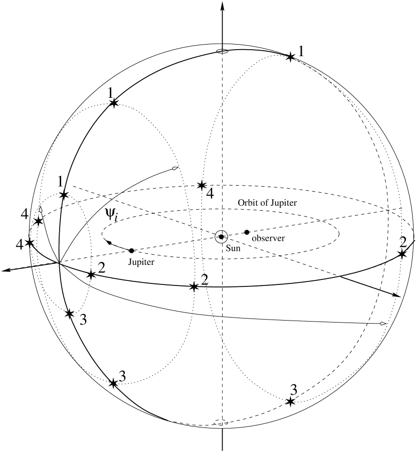
Figure 4: Geometry for the self-consistency test. The observer is aligned along the Sun-Jupiter direction and for each angular distance $\psi$ four stars at symmetric positions with respect to the perturbing bodies are considered. In RAMOD4 the spherical symmetry is broken by the orbital motion of the bodies. In the figure only the orbit of Jupiter is highlighted, while that of the Sun cannot be drawn because of its small radius.

Table 1: Summary of the results for the self-consistency test. The first column shows the angular distance $\psi$ from the Sun (in degrees), the second column is the mass ratio of the planet and the Sun, $\delta\psi$ is the deflection (identical in all the four quadrants) obtained from RAMOD3 measured in arcseconds, the $\Delta(\delta\psi_{i})$ are the differences in $\mu\mathrm{as}$ between the deflection of RAMOD4 and RAMOD3 in the $i$-th quadrant, according to the schema depicted in figure 4.

$\psi\;(\mathrm{deg)}$	$m_{J}/m_{\odot}$	$\delta\psi$	$\Delta(\delta\psi_{1}),\Delta(\delta\psi_{3})$	$\Delta(\delta\psi_{2})$	$\Delta(\delta\psi_{4})$
$\simeq 0.27(\equiv 1\>R_{\odot})$	$10^{-3}$	$1.7509921$	$<10^{-1}$	$-13.2$	$13.2$
$"$	$10^{-4}$	$1.7507492$	$"$	$-1.3$	$1.3$
$"$	$10^{-5}$	$1.7507249$	$"$	$-0.1$	$0.1$
$"$	$10^{-6}$	$1.7507224$	$"$	$<10^{-1}$	$<10^{-1}$
$1$	$10^{-3}$	$0.4667362$	$"$	$-1.0$	$1.0$
$"$	$10^{-4}$	$0.4666715$	$"$	$-0.1$	$0.1$
$"$	$10^{-5}$	$0.4666651$	$"$	$<10^{-1}$	$<10^{-1}$
$2$	$10^{-3}$	$0.2333501$	$"$	$-0.2$	$0.2$
$"$	$10^{-4}$	$0.2333177$	$"$	$<10^{-1}$	$<10^{-1}$
$5$	$10^{-3}$	$0.0932902$	$"$	$<10^{-1}$	$<10^{-1}$

Self-consistency test.

Let us remind the original configuration of the spherical symmetry test done in RAMOD3, i.e. the self-consistency test (de Felice et al.,, 2004). In the cited paper we imposed the condition that the Sun were the only source of gravity and looked for the symmetry of the light deflections with respect to its center. Here we considered the similar case where, however, the perturbing field is that of the point-like masses of the Sun and Jupiter aligned with the observer; the geometrical configuration relative to this test is sketched in figure 4. Here we considered an observer at 1 AU from the Sun and 6.2 AU from Jupiter, and a set of stars placed at different angular distances $\psi$ from the Sun. For each $\psi$ we have taken four stars symmetrical positioned with respect to the instantaneous axis joining the observer to the Sun and Jupiter: the anisotropy among the deflections are expected to be more evident on the orbital plane of the two bodies. The results are reported in table 1, where we can see that both our predictions were satisfied, i.e.:

1. $\delta\psi_{1}$ and $\delta\psi_{3}$ are equal and coincident with those of RAMOD3 to $0.1\,\mu$as, while $\delta\psi_{2}\neq\delta\psi_{4}$ and different from those of RAMOD3;

2. the differences between $\delta\psi_{2}$ and $\delta\psi_{4}$ in RAMOD3 and RAMOD4 are of the expected order ($\simeq 13.2\>\mu\mathrm{as}$ for Sun-grazing rays and quickly falling below the $0.1\>\mu\mathrm{as}$ for angular distances $\psi\gtrsim 5$ deg);

3. the deflection is greater in the case where the Sun trajectory is approaching the photon path and smaller in the opposite side, where it is getting farther from it.

As a final verification for this self-consistency test, we repeated several times the same run but with a less massive planet. Obviously, we expected that, as the mass of the planet decreases, the results tend to those of the perfectly symmetric case: i.e. as $m_{\mathrm{jup}}\rightarrow 0$, the velocities of Jupiter and the Sun go to zero as well. Table 1 shows that the deflections are perfectly symmetric down to the $0.1\>\mu\mathrm{as}$ level when $m_{\mathrm{planet}}=10^{-3}m_{\mathrm{jup}}$.

Codes	Contributions
	$r(t)$	$r_{\mathrm{ret}}$	$v$
R3a	Yes	No	No
R3b	Yes	Yes	No
R4b	Yes	Yes	Yes

Table 2: Schematic representation of the different codes under comparisons. While R4 stands for the one that implements RAMOD4, R3a and R3b indicate different “flavors” of a RAMOD3-like code. Among the specific contributions, $r(t)$ means that we consider the equations of motion of RAMOD3, but taking into account the planetary motion in the sense described in the main text of the article; $r_{\mathrm{ret}}$ that, when calculating the distances (and the velocities) of the perturbing bodies from the photon which enter the metric coefficients, we consider the finite gravity speed (i.e. the reduced distance); finally, $v$ means that the equations of motion are those of RAMOD4 and that the metric is complete with its $1/c^{3}$ terms depending explicitly on the velocity of the perturbing bodies. In the original RAMOD3 code, which strictly implements the $1/c^{2}$ model and its hypotheses, none of these contributions are taken into account, while all of them are present in R4 at its full extent.

Disentangling the non-stationary space-time effects.

To this purpose we have checked RAMOD4 against different (somewhat hybrid) versions of the RAMOD framework, where, according to table 2, they will be called in the following:

1. R4: the code implementing the full RAMOD4 model;

2. R3b: the R4 code without the $1/c^{3}$ terms depending explicitly on the velocity of the perturbing bodies. In this case the master equations are reconducted to that of RAMOD3, whereas the reduced distances are still fully considered and the planets are moving along their orbits;

3. R3a: the R4 code without both the velocity-dependent terms and the reduced distances. In this case we consider, for each step of integration, a different position of each perturbing body. These positions are those for circular orbits at time $t_{i}$ of the $i$-th step of integration.

The importance of these tests, as said above, is numerical rather than physical since, e.g., the exclusion of the reduced distance cannot be acceptable in a strictly physical sense. It can be important, however, if one is interested in the practical implementation of a particular code: in this case what one should care about is the efficiency and the speed of the code given the required level of accuracy. A similar comparison was done by Klioner and Peip, (2003) for the model in Klioner, (2003), and in this sense the R3a and R3b cases resembles cases $P_{1}$ and $P^{\prime}_{3}$ of that paper, respectively.

In these tests we considered only the presence of the Sun and Jupiter, since all the planets can be added with no loss of generality in the same way as Jupiter. Two cases have been taken into account, as sketched in figure 5: (i) when the observer lies between the Sun and Jupiter, or (ii) when the Sun is between the observer and Jupiter. The first case allows to evaluate the specific contribution of the Sun and of Jupiter separately, putting them in opposite direction with respect to the observer, while the second is more sensitive in order to investigate at which level of accuracy the model feels the non-linearity of the superimposition of the two-body gravitational field.

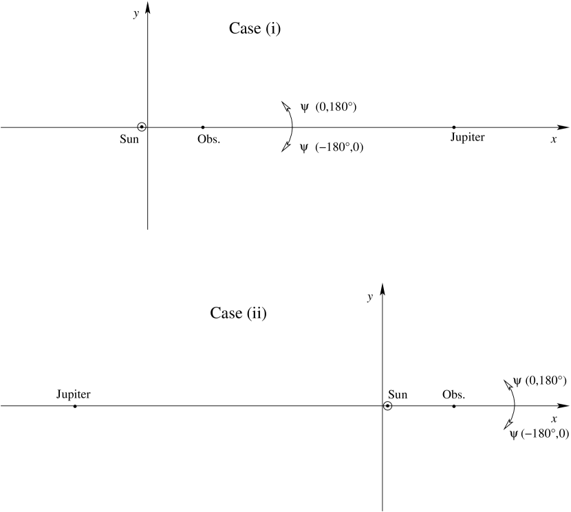
Figure 5: Sketch of the geometrical configurations for the tests using the codes R4, R3b and R3a.

For both of the cases the results indicate that:

1. the differences between R3a and R4 are $\sim 4.5\>\mu\mathrm{as}$ at most, meaning that the influence of the fixed planetary positions are of $\lesssim 9\>\mu\mathrm{as}$. In particular, the greatest effect is for photons which graze Jupiter ($\sim 4.5\>\mu\mathrm{as}$) instead of the Sun ($\lesssim 0.3\>\mu\mathrm{as}$);

2. the differences between R3b and R4 are tipically less than those between R3a and R4, but their ratios vary according to the geometrical configuration of the perturbing bodies and the observer, going from, e.g., one order of magnitude to about $1$. Once again the greatest difference occurs in the case of photons grazing Jupiter, as it should be expected since its velocity is far bigger than that of the Sun, and it amounts to $\sim 1.8\>\mu\mathrm{as}$ while the Sun contributes with $\sim 10^{-1}\>\mu\mathrm{as}$ at most.

This means that one should be careful at choosing the code integrating the photons’ geodesics. Optimizations are possible, but they must be tuned with the geometrical configuration of the perturbing bodies.

Table 3: Excerpts from the results of the code-comparing test. This table is for the (i) case, in which the observer lies between the Sun and Jupiter. The first column gives the angle that the photon’s incoming direction forms with the $x$ axis counted counter-clockwise in the range $[-180^{\circ},180^{\circ})$ as sketched in figure 5. The next three columns contain the deflections given by the three codes (in arcseconds) and the fifth and sixth columns give the difference in $\mu\mathrm{as}$ of R3b and R3a with R4 respectively.

$\psi\;(\mathrm{deg)}$		$\delta\psi\;\mathrm{(arcsec)}$		$(\delta\psi_{\mathrm{R4}}-\delta\psi_{\mathrm{R3b}})\;(\mu\mathrm{as})$	$(\delta\psi_{\mathrm{R4}}-\delta\psi_{\mathrm{R3a}})\;(\mu\mathrm{as})$
	R4	R3b	R3a
179.7334367	1.75073792543	1.75073781174	1.75073764027	0.11369	0.28516
179.4668735	0.87535666435	0.87535660782	0.87535652209	0.05653	0.14226
178.4006205	0.29176702035	0.29176700193	0.29176697336	0.01842	0.04699
160.1792868	0.02330937402	0.02330937317	0.02330937094	0.00086	0.00308
120.1507651	0.00707469758	0.00707469781	0.00707469723	-0.00024	0.00035
80.1222434	0.00342350034	0.00342350079	0.00342350051	-0.00045	-0.00018
40.0937217	0.00148347654	0.00148347699	0.00148347671	-0.00044	-0.00016
5.7835603	0.00018740032	0.00018739969	0.00018739782	0.00062	0.00250
0.03912	0.0025469505	0.0025471242	0.00254738571	-0.17370	-0.43521
0.01956	0.00480767427	0.00480800257	0.00480849601	-0.32830	-0.82174
0.00652	0.01176284745	0.01176365151	0.01176485859	-0.80406	-2.01115
-0.00652	0.0263647168	0.02636291438	0.02636020825	1.80242	4.50856
-0.01956	0.0062147205	0.00621429593	0.00621365819	0.42457	1.06231
-0.03912	0.00289458627	0.00289438879	0.00289409164	0.19749	0.49463
-5.7835603	0.00018738265	0.00018738327	0.00018738515	-0.00062	-0.00250
-40.0937217	0.00148347648	0.00148347603	0.00148347631	0.00044	0.00016
-80.1222434	0.00342350043	0.00342349998	0.00342350025	0.00045	0.00018
-120.1507651	0.0070746969	0.00707469666	0.00707469725	0.00024	-0.00035
-160.1792868	0.02330936614	0.02330936699	0.02330936922	-0.00085	-0.00308
-178.4006205	0.29176611396	0.29176613238	0.29176616095	-0.01842	-0.04699
-179.4668735	0.87534872947	0.87534878599	0.87534887173	-0.05653	-0.14226
-179.7334367	1.75070641203	1.75070652571	1.75070669718	-0.11368	-0.28515

Table 4: Excerpts from the results of the code-comparing test. This table is for the (ii) case, in which the Sun is between the observer and Jupiter. The table headings are the same as in table 3.

$\psi\;(\mathrm{deg)}$		$\delta\psi\;\mathrm{(arcsec)}$		$(\delta\psi_{\mathrm{R4}}-\delta\psi_{\mathrm{R3b}})\;(\mu\mathrm{as})$	$(\delta\psi_{\mathrm{R4}}-\delta\psi_{\mathrm{R3a}})\;(\mu\mathrm{as})$
	R4	R3b	R3a
179.7334367	1.75097892390	1.75097901914	1.75097916265	-0.09525	-0.23876
179.4668735	0.87548418970	0.87548423717	0.87548430900	-0.04746	-0.11930
178.4006205	0.29181111968	0.29181113523	0.29181115918	-0.01554	-0.03950
160.1792868	0.02331311678	0.02331311760	0.02331311946	-0.00082	-0.00268
120.1507651	0.00707631845	0.00707631834	0.00707631882	0.00011	-0.00036
80.1222434	0.00342512778	0.00342512747	0.00342512763	0.00032	0.00016
40.0937217	0.00148624154	0.00148624114	0.00148624118	0.00040	0.00037
5.7835603	0.00020574544	0.00020574502	0.00020574502	0.00043	0.00042
0.0391200	0.00000139069	0.00000139027	0.00000139027	0.00043	0.00043
-0.0391200	0.00000139027	0.00000139069	0.00000139069	-0.00043	-0.00043
-5.7835603	0.00020574502	0.00020574544	0.00020574544	-0.00043	-0.00042
-40.0937217	0.00148624118	0.00148624158	0.00148624155	-0.00040	-0.00037
-80.1222434	0.00342512767	0.00342512799	0.00342512783	-0.00032	-0.00016
-120.1507651	0.00707631909	0.00707631920	0.00707631873	-0.00011	0.00036
-160.1792868	0.02331312349	0.02331312268	0.02331312081	0.00082	0.00268
-178.4006205	0.29181187997	0.29181186441	0.29181184044	0.01555	0.03952
-179.4668735	0.87549084388	0.87549079633	0.87549072436	0.04755	0.11952
-179.7334367	1.75100533870	1.75100524311	1.75100509907	0.09560	0.23963

6 Conclusions

Aim of modern relativistic astrometry is to produce a three dimensional rendering of our Galaxy with an accuracy of one $\mu\mathrm{as}$ in the measurements of angles. In order to reach this goal one needs an appropriate algorithm to trace back to their emission space-time points the light signals which are intercepted by a suitable observational device.

In the near future, one of such devices will be the astrometric satellite Gaia which will orbit the Sun from nearby the Sun-Earth outer Lagrangian point $L_{2}$. The expected accuracy of the satellite observations requires that one should treat the light propagation through the Solar System in a general relativistic framework and consider the general relativistic effects induced by the bodies of the Solar System up to the order of $1/c^{3}$.

Our strategy was to construct a series of models with increasing generality and complexity, exploiting each of them as a test-bed for the more advanced one. Our last model accurate to $1/c^{3}$ is RAMOD4. As previously discussed, we first compared RAMOD4 to its less accurate predecessor RAMOD3, which was accurate to $1/c^{2}$. With a suitable handling of the items considered in the model, we are able to highlight the relative importance of the individual sources of relativistic perturbations and judge about their physical relevance.

Our first conclusion is that RAMOD4 behaves as expected with respect to RAMOD3, that is, the differences between the two models are at the expected level of $\sim 10~{}\mu\mathrm{as}$. So this work successfully completes the series of models from a theoretical point of view and represents a launching platform to deduce with a completely numerical algorithm the astrometric parameters of a celestial object from a well-defined set of relativistically measured quantities.

This model, however, is part of a broader project whose completion requires its implementation into a feasible and efficient structure for the data reduction of the Gaia mission. In this sense, the practical application of this model requires also to investigate the specific ways of implementing it with respect to the accuracy goals of the mission. For this reason, then, we tried to single out the different contribution which come out together from the motion of the perturbing bodies, and evaluate them separately. We found that the contribution to the total deflection coming from the velocity-induced terms of the metric is generally smaller than that of the reduced distance, but not negligible at the $0.1~{}\mu\mathrm{as}$ level. The former one can in fact reach a maximum amount of $\sim 1.8\>\mu\mathrm{as}$ while the latter goes up to $\sim 4.5\>\mu\mathrm{as}$. Both these cases, and the greatest differences with RAMOD3, come out when the photon is grazing Jupiter, while the Sun contributes up to less than $0.3~{}\mu\mathrm{as}$ that is one order of magnitude lower.

Given the unprecedented accuracy reachable by Gaia-like missions, several new relativistic tests related to the light propagation in a non-stationary gravitational field could be carried out. From this point of view it is advisable to create a cross-check framework of models to validate the relativistic outputs induced by the modeling itself at the microarcsecond level. In fact, our Relativistic Astrometric Model naturally confronts itself with the works of Kopeikin, Schäfer and Mashhoon (Kopeikin and Schäfer,, 1999; Kopeikin and Mashhoon,, 2002) and Klioner, (2003). While the latter stems from the general formulation of the former conforming to its basic tenets, our model responds to an inherently different strategy. As far as the astrometric problem is concerned, in the Kopeikin-Schäfer and Klioner approach the light ray is reconstructed as a sum of terms which allows for a direct evaluation of the individual relativistic effects induced by the gravitating bodies that the light ray is expected to encounter on its way. Each relativistic effect enters as a perturbation of the light ray trajectory and is treated to a sufficiently high order (not less than $1/c^{3}$) to cope with the accuracy expected from Gaia’s observations. Our model instead aims to determine a full solution for the light trajectory which naturally includes, in a curved space-time, all the individual effects; the latters are somewhat hidden in the covariant formalism of our approach and directly contribute to the solutions of our master equations. Evidently any specific effect one is interested to explore can be independently deduced from our formalism as a branch output, once we adapt the master equation to a required specific case.

Although our model and Klioner’s are of comparable accuracy as it can be deduced from individual tests, the overall structure of Klioner’s model makes it ready to handle the reduction of a large number of observational data in a computational efficient way; nevertheless we are confident that our model will soon reach the same versatility and operate as an essential tool of verification. However, the general covariant formulation of our model, including the complete relativistic treatment of the satellite attitude (Bini and de Felice,, 2003; Bini et al.,, 2003), represents a well defined framework where any desired advancement in the light tracing problem using astrometric data is contemplated.

Appendix A The attitude frame

Given the tetrad adapted to the local barycentric observer $\{\mbox{\boldmath$u$\unboldmath},\mbox{\boldmath$\lambda$\unboldmath}_{\hat{a}}\}$ (Bini and de Felice,, 2003), first we identify the spatial direction to the Sun as seen in the local BCRS and at a general point on the satellite’s space-time trajectory. Then we construct the triad $\{{\mbox{\boldmath$\lambda_{\hat{a}}$\unboldmath}}{}{{}_{(\mathrm{s})}}\}$ where one of those vectors identifies the Sun direction. Clearly the set $\{\mbox{\boldmath$u$\unboldmath},{\mbox{\boldmath$\lambda$\unboldmath}_{\hat{a}}}{}{{}_{(\mathrm{s})}}\}$ forms still an orthonormal tetrad adapted to the local barycentric observer.

As second step, we boost the vectors of the triad $\{{\mbox{\boldmath$\lambda$\unboldmath}_{\hat{a}}}{}{{}_{(\mathrm{s})}}\}$ to the satellite rest frame; remembering that $\mbox{\boldmath$u$\unboldmath}^{\prime}$ is the vector field tangent to Gaia’s world-line we have (Jantzen et al.,, 1992):

$${\lambda_{\hat{a}}^{\alpha}}{}{{}_{(\mathrm{bs})}}=P(u^{\prime})^{\alpha}{}_{\sigma}\left[{\lambda_{\hat{a}}^{\sigma}}{}{{}_{(\mathrm{s})}}-\frac{\gamma}{\gamma+1}\nu^{\sigma}\left(\nu^{\rho}{\lambda_{\rho\hat{a}}}{}{{}_{(\mathrm{s})}}\right)\right]_{{\hat{a}}=1,2,3}.$$ (A1)

The tetrad $\{{\mbox{\boldmath$\lambda$\unboldmath}_{\hat{0}}}{}{{}_{(\mathrm{bs})}}\equiv\mbox{\boldmath$u$\unboldmath}^{\prime},{\mbox{\boldmath$\lambda$\unboldmath}_{\hat{a}}}{}{{}_{(\mathrm{bs})}}\}$ represents a CoMRS Sun-locked frame, i.e. a Center-of-Mass Reference System (Bastian,, 2004) comoving with the satellite and with one axis fixed toward the Sun at any point of its Lissajous orbit around $L_{2}$. The relation between the components $\nu^{\alpha}$ of the spatial four-velocity $\nu$ and the components $\beta^{i}$ appearing in (45) is easily established from (45) itself and (46) and reads:

$$\nu^{\alpha}=\frac{1}{\gamma}\left[u^{\prime 0}\left(\beta_{i}\delta^{i\alpha}+\delta^{0\alpha}\right)-u^{\alpha}\gamma\right].$$ (A2)

The explicit expressions of the components of these vectors relative to the BCRS are reported in Bini et al., (2003).

The triad components are given by

$${\lambda_{\hat{1}}^{t}}{}{{}_{(\mathrm{bs})}} = \Psi(1+\frac{1}{2}\beta^{2}+3U)+\cos\theta\cos\phi h_{01}+\cos\theta\sin\phi h_{02}+\sin\theta h_{03}$$ (A3)

$${\lambda_{\hat{1}}^{x}}{}{{}_{(\mathrm{bs})}} = \cos\theta\cos\phi(1-U)+\frac{1}{2}\beta_{1}\Psi$$ (A4)

$${\lambda_{\hat{1}}^{y}}{}{{}_{(\mathrm{bs})}} = \cos\theta\sin\phi(1-U)+\frac{1}{2}\beta_{2}\Psi$$ (A5)

$${\lambda_{\hat{1}}^{z}}{}{{}_{(\mathrm{bs})}} = \sin\theta(1-U)+\frac{1}{2}\beta_{3}\Psi$$ (A6)

$${\lambda_{\hat{2}}^{t}}{}{{}_{(\mathrm{bs})}} = \Phi(1+\frac{1}{2}\beta^{2}+3U)-\sin\phi h_{01}+\cos\phi h_{02}$$ (A7)

$${\lambda_{\hat{2}}^{x}}{}{{}_{(\mathrm{bs})}} = -\sin\phi(1-U)+\frac{1}{2}\beta_{1}\Phi$$ (A8)

$${\lambda_{\hat{2}}^{y}}{}{{}_{(\mathrm{bs})}} = \cos\phi(1-U)+\frac{1}{2}\beta_{2}\Phi$$ (A9)

$${\lambda_{\hat{2}}^{z}}{}{{}_{(\mathrm{bs})}} = -\frac{1}{2}\beta_{3}\Phi$$ (A10)

$${\lambda_{\hat{3}}^{t}}{}{{}_{(\mathrm{bs})}} = \Theta(1+\frac{1}{2}\beta^{2}+3U)-\sin\theta(\cos\phi h_{01}+\sin\phi h_{02})+\cos\theta h_{03}$$ (A11)

$${\lambda_{\hat{3}}^{x}}{}{{}_{(\mathrm{bs})}} = -\cos\theta\sin\theta(1-U)+\frac{1}{2}\beta_{1}\Theta$$ (A12)

$${\lambda_{\hat{3}}^{y}}{}{{}_{(\mathrm{bs})}} = -\sin\theta\sin\phi(1-U)+\frac{1}{2}\beta_{2}\Theta$$ (A13)

$${\lambda_{\hat{3}}^{z}}{}{{}_{(\mathrm{bs})}} = \cos\theta(1-U)+\frac{1}{2}\beta_{3}\Theta$$ (A14)

where

$$\Psi \equiv \cos\theta\cos\phi\beta_{1}+\cos\theta\sin\theta\beta_{2}+\sin\theta\beta_{3}$$ (A15)

$$\Phi \equiv -\sin\phi\beta_{1}+\cos\phi\beta_{2}$$ (A16)

$$\Theta \equiv -\sin\theta(\cos\phi\beta_{1}+\sin\phi\beta_{2})+\cos\theta\beta_{3}.$$ (A17)

Here $2U=h_{00}$ and the angles $\theta$ and $\phi$ are defined as

$$\phi=\tan^{-1}\frac{y^{\prime}_{\odot}}{x^{\prime}_{\odot}},\qquad\theta=\tan^{-1}\frac{z^{\prime}_{\odot}}{\sqrt{x^{\prime}{}_{\odot}^{2}+y^{\prime}{}_{\odot}^{2}}}$$ (A18)

where $x^{\prime}_{\odot}$, $y^{\prime}_{\odot}$ and $z^{\prime}_{\odot}$ fix the spatial coordinate position of the Sun relative to the satellite at each time $t$; clearly in terms of the coordinates of the Sun and the satellite they are defined as

$$x^{\prime}_{\odot}=x_{\odot}-x_{0}\qquad y^{\prime}_{\odot}=y_{\odot}-y_{0}\qquad z^{\prime}_{\odot}=z_{\odot}-z_{0}.$$ (A19)

See Bini et al., (2003) for details. It is straightforward although tedious to show analytically that $\bar{\ell}_{0}^{k}$ as solution of (48) with triad (49), (4), (4) is unitary as expected.

Appendix B Explicit form for the master equations

Adopting the metric given in (25), the differential equations for the spatial components $\bar{\ell}^{i}$ of the null geodesic take the following form:

$$\frac{\mathrm{d}^{2}x^{k}}{\mathrm{d}t^{2}}+\sum_{a} \left\{\displaystyle{\frac{2m^{(a)}}{{r^{(a)}}^{2}}}\right. \left[\frac{1}{2}\left(\frac{\mathrm{d}x^{k}}{\mathrm{d}t}\frac{\partial r^{(a)}}{\partial t}+\frac{\partial r^{(a)}}{\partial x^{k}}\left(1+\mathbf{v}^{(a)}\cdot\mathbf{n}^{(a)}\right)\right)\left(\left(\frac{\mathrm{d}x}{\mathrm{d}t}\right)^{2}+\left(\frac{\mathrm{d}y}{\mathrm{d}t}\right)^{2}+\left(\frac{\mathrm{d}z}{\mathrm{d}t}\right)^{2}\right)\right.$$

$$-\left(\frac{3}{2}\frac{\mathrm{d}x^{k}}{\mathrm{d}t}\left(1+\mathbf{v}^{(a)}\cdot\mathbf{n}^{(a)}\right)-2v^{(a)}_{k}\right)\left(\frac{\mathrm{d}x}{\mathrm{d}t}\frac{\partial r^{(a)}}{\partial x}+\frac{\mathrm{d}y}{\mathrm{d}t}\frac{\partial r^{(a)}}{\partial y}+\frac{\mathrm{d}z}{\mathrm{d}t}\frac{\partial r^{(a)}}{\partial z}\right)$$

$$\left.-\frac{\mathrm{d}x^{k}}{\mathrm{d}t}\frac{\partial r^{(a)}}{\partial t}+\frac{1}{2}\frac{\partial r^{(a)}}{\partial x^{k}}\left(1+\mathbf{v}^{(a)}\cdot\mathbf{n}^{(a)}\right)-2\frac{\partial r^{(a)}}{\partial x^{k}}\left(\frac{\mathrm{d}x}{\mathrm{d}t}v^{(a)}_{x}+\frac{\mathrm{d}y}{\mathrm{d}t}v^{(a)}_{y}+\frac{\mathrm{d}z}{\mathrm{d}t}v^{(a)}_{z}\right)\right]+$$

$$\displaystyle{\frac{2m^{(a)}}{r^{(a)}}} \left[\frac{3}{2}\frac{\mathrm{d}x^{k}}{\mathrm{d}t}\left(\frac{\mathrm{d}x}{\mathrm{d}t}\frac{\partial\left(\mathbf{v}^{(a)}\cdot\mathbf{n}^{(a)}\right)}{\partial x}+\frac{\mathrm{d}y}{\mathrm{d}t}\frac{\partial\left(\mathbf{v}^{(a)}\cdot\mathbf{n}^{(a)}\right)}{\partial y}+\frac{\mathrm{d}z}{\mathrm{d}t}\frac{\partial\left(\mathbf{v}^{(a)}\cdot\mathbf{n}^{(a)}\right)}{\partial z}\right)-\right.$$

$$\left.\frac{1}{2}\frac{\partial\left(\mathbf{v}^{(a)}\cdot\mathbf{n}^{(a)}\right)}{\partial x^{k}}\left(\left(\frac{\mathrm{d}x}{\mathrm{d}t}\right)^{2}+\left(\frac{\mathrm{d}y}{\mathrm{d}t}\right)^{2}+\left(\frac{\mathrm{d}z}{\mathrm{d}t}\right)^{2}+1\right)\right]-$$

$$\displaystyle{\frac{4m^{(a)}}{r^{(a)}}} \left.\frac{\mathrm{d}\mathbf{r}}{\mathrm{d}t}\cdot\left(\nabla\times\mathbf{v}^{(a)}\right)_{k}\right\}=0$$

In the case of circular orbits, the last line of each equation disappears since $\nabla\times\mathbf{v}^{(a)}=0$ in this case. Moreover with straightforward calculations, similar to those appeared in section 5.1, one can easily find that

$$\mathbf{v}^{(a)}\cdot\mathbf{n}^{(a)}=\frac{\omega}{r^{(a)}}\left[(yx^{(a)}-xy^{(a)})\cos(\omega r^{(a)})+(xx^{(a)}+yy^{(a)})\sin(\omega r^{(a)})\right]$$

and

$$\frac{\partial\left(\mathbf{v}^{(a)}\cdot\mathbf{n}^{(a)}\right)}{\partial x^{k}} = \frac{\omega}{r^{(a)}}\left[\cos(\omega r^{(a)})(\delta^{y}_{i}x^{(a)}-\delta^{x}_{i}y^{(a)})+\sin(\omega r^{(a)})(\delta^{x}_{i}x^{(a)}+\delta^{y}_{i}y^{(a)})\right]+$$

$$+ (\partial_{i}r^{(a)})\left\{\frac{\omega^{2}}{r^{(a)}}\left[-(yx^{(a)}-xy^{(a)})\sin(\omega r^{(a)})+(xx^{(a)}+yy^{(a)})\cos(\omega r^{(a)})\right]-\frac{\mathbf{v}^{(a)}\cdot{\mathbf{r}^{(a)}}}{r^{(a)2}}\right\}.$$

where all the coordinates of the planets are at time $t$, while $r^{(a)}$ and $\mathbf{v}^{(a)}$ are at time $t^{\prime}$ (this means that one should replace $r^{(a)}$ with its approximation of eq.(69).

References

Bastian, (2004)
Bastian, U. (2004).
Reference System, Conventions and Notations for Gaia.
Research Note GAIA-ARI-BAS-003, GAIA livelink.
Bini et al., (2003)
Bini, D., Crosta, M. T., and de Felice, F. (2003).
Orbiting frames and satellite attitudes in relativistic astrometry.
Class. Quantum Grav., 20:4695–4706.
Bini and de Felice, (2003)
Bini, D. and de Felice, F. (2003).
Ray tracing in relativistic astrometry: the boundary value problem.
Class. Quantum Grav., 20:2251–2259.
de Felice et al., (2001)
de Felice, F., Bucciarelli, B., Lattanzi, M. G., and Vecchiato, A.
(2001).
General relativistic satellite astrometry. II. Modeling parallax
and proper motion.
Astron. Astrophys., 373:336–344.
de Felice and Clarke, (1990)
de Felice, F. and Clarke, C. J. S. (1990).
Relativity on curved manifolds.
Cambridge University Press.
de Felice et al., (2004)
de Felice, F., Crosta, M. T., Vecchiato, A., Lattanzi, M. G., and
Bucciarelli, B. (2004).
A General Relativistic Model of Light Propagation in the
Gravitational Field of the Solar System: The Static Case.
Astrophys. J., 607:580–595.
de Felice et al., (1998)
de Felice, F., Lattanzi, M. G., Vecchiato, A., and Bernacca, P. L.
(1998).
General relativistic satellite astrometry. I. A non-perturbative
approach to data reduction.
Astron. Astrophys., 332:1133–1141.
IAU, (2000)
IAU (2000).
Definition of Barycentric Celestial Reference System and Geocentric
Celestial Reference System.
IAU Resolution B1.3 adopted at the 24th General Assembly, Manchester,
August 2000.
Jantzen et al., (1992)
Jantzen, R. T., Carini, P., and Bini, D. (1992).
The many faces of gravitoelectromagnetism.
Ann. Phys., 215:1–50.
Klioner, (2003)
Klioner, S. A. (2003).
A Practical Relativistic Model for Microarcsecond Astrometry in
Space.
Astron. J., 125:1580–1597.
Klioner and Peip, (2003)
Klioner, S. A. and Peip, M. (2003).
Numerical simulations of the light propagation in the gravitational
field of moving bodies.
Astron. Astrophys., 410:1063–1074.
Kopeikin and Mashhoon, (2002)
Kopeikin, S. M. and Mashhoon, B. (2002).
Gravitomagnetic effects in the propagation of electromagnetic waves
in variable gravitational fields of arbitrary-moving and spinning bodies.
Phys. Rev. D, 65:64025.
Kopeikin and Schäfer, (1999)
Kopeikin, S. M. and Schäfer, G. (1999).
Lorentz Covariant Theory of Light Propagation in Gravitational
Fields of Arbitrary Moving Bodies.
Phys. Rev. D, 60:124002.
Le Poncin-Lafitte et al., (2004)
Le Poncin-Lafitte, C., Linet, B., and Teyssandier, P. (2004).
World function and time transfer: general post-Minkowskian
expansions.
Class. Quantum Grav., 21:4463–4483.
Misner et al., (1973)
Misner, C. W., Thorne, K. S., and Wheeler, J. A. (1973).
Gravitation.
San Francisco: W.H. Freeman and Co.
Turon et al., (2005)
Turon, C., O’Flaherty, K. S., and Perryman, M. A. C., editors (2005).
The Three-Dimensional Universe with Gaia.
Weinberg, (1972)
Weinberg, S. (1972).
Gravitation and Cosmology: Principles and Applications of the
General Theory of Relativity.
Gravitation and Cosmology: Principles and Applications of the General
Theory of Relativity, by Steven Weinberg, pp. 688. ISBN
0-471-92567-5. Wiley-VCH , July 1972.