First results from the Pierre Auger Observatory

Abstract

We review in these notes the status of the construction of the Pierre Auger Observatory and present the first Physics results, based on the data collected during the first year and a half of operation. These results are preliminary, once the work to understand the systematics of the detectors are still underway. We discuss the cosmic ray spectrum above 3 EeV, based on the measurement done using the Surface Detector and the Fluorescence Detector, both, components of the observatory. We discuss, as well, the search for anisotropy near the Galactic Center and the limit on the photon fraction at the highest energies.

I Introduction

The cosmic ray spectrum, measured at the top of the atmosphere covers a huge range in energy, going from 10 MeV to energies above $10^{20}$ eV, with a differential flux that spans 31 decades [1]. The techniques to survey this spectrum goes from instruments aboard satellite flights, balloon borne detectors, to counters that monitor the fluxes of neutrons and muons at the Earth surface, and at higher energies to wide area arrays of particle detectors. The spectrum can be divided roughly into four regions with very distinct behavior. The first one, with energies below 1 GeV, has a very distinctive character from the rest of it. Its shape and cut-off is strongly dependent on the phase of the solar cycle, a phenomenon known as solar modulation. Actually, there is an inverse correlation between the intensity of cosmic rays at the top of the atmosphere and the level of the solar activity [2, 3].

The region above 1 GeV show a spectrum with a power law dependence, $N(E)$ d$E=K~{}E^{-x}$ d$E$, where the spectral index $x$ varies as $2.7~{}<~{}x~{}<~{}3.2$. The region between 1 GeV and the knee region at $4\times 10^{15}$ eV, is characterized by an index $x~{}\simeq~{}2.7$. These cosmic rays most likely are produced at supernova explosions and their remnants [4]. At the knee ($4\times 10^{15}$ eV) the power law index steepens to 3.2 until the so called ankle, at $5\times 10^{18}$ eV. The origin of the cosmic rays in this region is less clear and subject of much conjecture. Above the ankle the spectrum flattens again to an index $x~{}\simeq~{}2.8$ and this is interpreted by many authors as a cross over from the steeper galactic component to a harder extra galactic source for the cosmic rays [5, 6].

The existence of cosmic rays with energies above $10^{20}$ eV presents a puzzling problem in high energy astrophysics. The first event of this class of phenomena was observed at the beginning of the 60’s by John Linsley at the Volcano Ranch experiment, in New Mexico [7, 8]. Since then, many events were detected, at different sites, using quite distinct techniques [9, 10, 11, 12, 13]. If those cosmic rays are common matter, that is, protons, nuclei or even photons, they undergo well known nuclear and electromagnetic processes, during their propagation through space. Their energies are degraded by the interaction with the cosmic radiation background (cmb), way before they reached the Earth [14, 15]. After travelling distances at the scale of 50 Mpc, their energies should be under $10^{20}$ eV, thus restricting the possible conventional astrophysical objects, which could be sources of them, and those should be easily localized through astronomical instruments. On the other hand, it is very difficult to explain the acceleration of charged particles, with energies up to $3~{}\times~{}10^{20}$ eV or even greater, on known astrophysical objects, by means of electromagnetic forces, the only conventional ones capable of long range and long periods of acceleration.

II The Pierre Auger Observatory

The Pierre Auger Observatory [16, 17] was designed to study the higher – above $10^{18}$ eV – end of the cosmic ray spectrum, with high statistics over the whole sky. The detectors are optimized to measure the energy spectrum, the directions of arrival and the chemical composition of the cosmic rays, using two complementary techniques, surface detectors (SD) based on Cherenkov radiators and fluorescence light detectors (FD). The complete project calls for two sites, one in the southern hemisphere, well ahead in its construction, and a northern site, in order to achive the homogeneous coverage of the whole sky, essential to pinpoint the sources of the ultra high-energy cosmic rays.

The southern site of the Observatory, located in the province of Mendoza, in Argentina, at the latitude 35^∘ South and longitude 69^∘ West, on a very flat plateau at 1 400 m above sea level, is bounded by the Andes Cordillera on the west. The region has a very clear sky, with little light pollution, essential for the operation of the fluorescence system. The main office of the observatory is located at the northern entrance of the City of Malargüe. The construction of this part of the detector should be completed on the second half of 2007. The layout of the site is shown in Figure 1, indicating the distribution of detectors already deployed and the position of the fluorescence buildings.

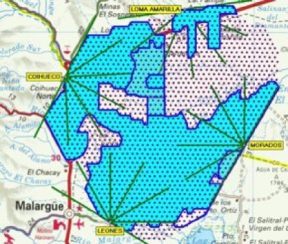
Figure 1: Layout of the Pierre Auger Observatory southern site showing the four FD telescopes (eyes). The dots represents the deployement location of the SD stations. The darker shade represents the area instrumented in July 2006. The FD eyes Los Leones, Los Morados and Coihueco are in full operation, while the construction of Loma Amarilla and its instrumentation should be completed by the end of 2006.

The construction of the northern site, in the southern part of the state of Colorado, at the United States, will start after the full completion of the southern site.

The initial phase of the Pierre Auger Observatory, the Engineering Array was built during the period 2000-2001. Then, 40 Cherenkov tanks were laid and instrumented, to test the components of the array and to prove the soundness of its design. They were set in a roughly hexagonal array, covering an area of 54 km². Two of the tanks, at the center of the array, were laid side by side, in order to cross calibrate their signals. Two prototype telescopes were installed on the Los Leones hill, overlooking this ground array. They were successfully tested during the southern summer of 2001-2002. The lessons learned in the Engineering Array lead to improvement in the final design of the detector components [18].

II.1 The Surface Detector

The Surface Detector (SD) is a ground array which spans an area of 3 000 km², with 1 600 stations set on a regular triangular grid, with 1 500 m separation between them. The stations communicate with the central base station through a radio link.

Each station at the SD is a cylindrical tank, filled with 12 000 l of purified water, operating as a Cherenkov light detector. The tanks are manufactured by rotational molding process, using a high density polyethylene resin, with 12.7 mm thick walls, opaque to external light. The walls have two layers, an external in the color beige, to minimize the environmental impact and reduce the heat absorption, and the internal black, with the addition of carbon black to the resin. The water is contained in a liner inside the tank, a bag made of a sandwich of polyolefin-Tyvek film. The Tyvek film has a high reflectivity to ultraviolet light and its role is to diffuse the UV Cherenkov light within the volume of water.

The tanks are prepared in the Assembly Building, just behid the Main campus building. The water purification plant produces enough water for 3 tanks per day, with a resistivity of 15 M$\Omega$ per cm. The tanks are manufactured in São Paulo, Brazil, and Buenos Aires and shipped all the way to Malargüe on flatbed trucks, carrying six tanks on a load. After preparation which includes the mounting of the electronic components, the cabling and fitting the internal Tyvek bag, the tanks are deployed on the field, on prepared ground, using 4-wheel drive vehicles.

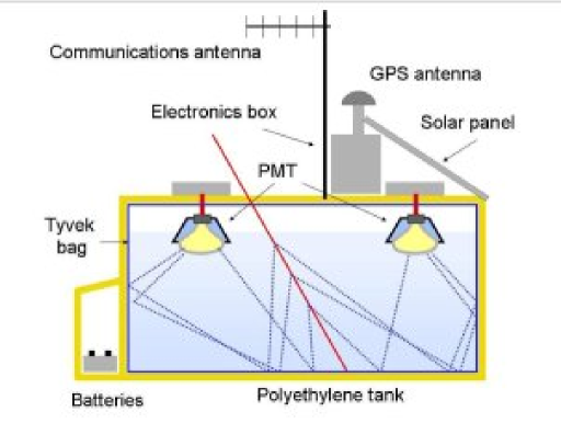
Figure 2: A schematic view of the Cherenkov water tanks, with the components indicated in the figure.

The Cherenkov light, diffused within the volume of water, is collected by three 20.3 cm diameter photomultiplier tubes (Photonis XP1805), set in a symmetric pattern on top of the tanks, facing downwards. This arrangement avoids the direct hit of the Cherenkov light, collecting a signal which is homogeneous and proportional to the length of charged tracks crossing the water. A schematic view of a SD station is shown in Figure 2.

The electronics for the detectors are housed in a box outside the tanks and communicate with a base station through a radio wlan, operating in the 915 MHz band. The stations are powered by a bank of two special 12 V batteries, which are fed by two solar panels of 55 W each. The time synchronization of the tanks is based on a gps system, capable of a time alignment precision of about 10 ns [19]. A 7 GHz microwave backbone links the base stations to the central data acquisition station (CDAS), at the campus of Malargüe in the southern site.

Each detector station has a two level trigger, a hardware implemented T1 and a software T2. The T1 trigger is decided in a PLD (Programmable Logical Device) [20], set with a threshold defined in terms of a vertical equivalent muon (VEM) crossing a tank, with a typical value of 1.75 VEM on a single 25 ns time bin, in coincidence at all working PMT’s. This trigger has a rate of about 100 Hz and is necessary to detect fast signals associated to the muons of horizontal showers. There is a second condition for T1, which is a time over threshold condition (ToT), requiring that the signal in 13 FADC bins out of a window of 120 bins are above a value of 0.2 VEM. The ToT trigger rate averages 1.6 Hz, dominated by coincidences of two muons and is efficient to select small signals away from the core of showers at the tail of the lateral distribution. T1 is adjusted so that its rate is about 100 Hz. T2 limits the trigger rate at each station to less than 20 Hz, so as not to saturate the radio bandwidth available. ToT triggers are promptly promoted to T2, while the threshold T1 are requested a tighter condition of 3.2 VEM in coincidence for the 3 PMTs. The event trigger (T3) is set at CDAS combining the triggers of contiguous individual stations. The requirement in the number of stations triggered sets the lower energy threshold. Typically, four stations are required for a threshold of 10¹⁹ eV. The communication between the central campus and the individual stations is bi-directional to allow the T3 trigger request the data to be downloaded to the CDAS system.

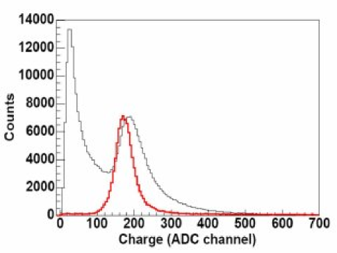
Figure 3: Typical histogram used in the calibration of the surface stations. This was taken from a prototype tank equipped with scintillation pads to select the component of the signal due to vertical muons. The hump of the experimental distribution of single muons is related to the signal due to a vertical incoming muon [21].

The calibration of the surface stations is done continuously. At every minute the histogram of low energy particles is taken, correspondinding roughly to about 100 000 events, mostly atmospheric muons coming from all angles into the detector. This calibration is performed in parallel to the data taking and at every 6 minutes this is sent to the central data acquisision system (CDAS) for monitoring [21]. Figure 3 shows a the histogram for a surface station, taken at a prototype detector.

The incoming angle of a shower is reconstructed from the timing of arrival of the signals in the tanks. The detectors have a large cross section even for a shower with very high zenith angle, so that Auger is quite sensitive to neutrinos [22, 23]. A highly inclined shower, originating from a hadronic cosmic ray, has a very characteristic signature, having lost a substantial part of its electromagnetic component, with only a core of energetic muons remaining. The muons arrive concentrated in time, generating signals with a very sharp peak. In contrast, a shower which has a large electromagnetic component is spread in time, with a much more complex structure.

II.2 The Fluorescence Detector

The Fluorescence Detector (FD) is composed of 4 eyes disposed on the vertices of a diamond-like configuration, with a separation of 65.7 km along the axis South-North (actually this axis is tilted by 19^∘ into Northeast) and 57.0 km in the West-East direction (tilted by 20^∘ into Southeast). They are at the periphery of the ground array and all stations of the SD are contained in the field of view (FOV) of the FD telescopes [24] (see Figure 1).

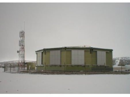
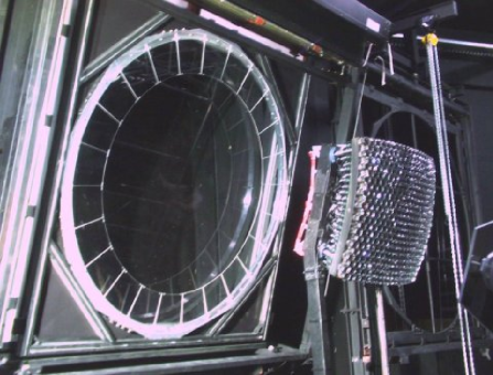
Figure 4: The Coihueco telescope building, with the shutters closed. Lower picture: The diaphragm of a telescope, with corrector rings. The picture shows the camera, with its 440 pixels facing the mirror.

Each eye has six independent telescopes, each with a field of view of $30^{\circ}$ in azimuth and $28.6^{\circ}$ in elevation, adding to a $180^{\circ}$ view of the array. Figure 4 shows the building of the Coihueco eye located on the west side of the array (see Figure 1). The fluorescence light is collected by a mirror with a radius of 3.4 m and reflected into a camera, located at the focal surface of the mirror. The telescopes use a Schmidt optics design to avoid coma aberration, with a diaphragm, at the center of curvature of the mirror, with an external radius of 0.85 m. The advantage of this scheme is to project a point of light in the sky into a reasonably homogeneous spot, at the focal surface, of 0.25^∘ radius.

The shape of the telescope mirror is a square with rounded corners with a side of 3.8 m. The radius of the diaphragm may be enlarged to 1.1 m, by adding a corrector lens annulus on the area with radius between 0.85 m and 1.1 m [25] (see Figure 4). The telescope, which is remotely operated, is protected from the environment by an external shutter and a MUG-6 UV transmitting filter, which reduces the light background.

The camera is composed by 440 pixels, each a hexagonal photomultiplier (Photonis XP3062), which monitors a solid angle of (1.5^∘)² projected onto the sky. The dead spaces between the photomultipliers is corrected by a reflective wedge device, called the Mercedes corrector, making the sky exposure very uniform.

The electronics of the FD detector was designed to be operated remotely and with flexibility to reprogram the trigger to accommodate non-standard physical processes which may show up. The trigger rate is not limited by the transmission band available. The FD communicates with the CDAS system through the 7 GHz microwave backbone, with a capacity of 34 Mbps throughput.

To be able to operate in hybrid mode the absolute time alignment with the Cherenkov water detector must be better than 120 ns. The trigger for each FD pixel is programmed to have a rate below 100 Hz, while a special processor, with a built-in pattern recognition algorithm, keeps the overall trigger rate below 0.1 Hz. The pixels are sampled and the signal digitized at every 100 ns. The first level trigger uses a boxcar type addition of the signal over a 1 $\mu$s bin and a pixel trigger set whenever this sum is 3 $\sigma$ above the background noise. An event is triggered whenever a set of 5 contiguous pixels are triggered with a time sequence associated [26].

The calibration of the camera is performed by exposing the PMTs to signals from calibrated light sources diffused from an aparatus mounted on the external window of the telescopes. The camera is illuminated uniformly and the gain of each PMT characterized [27, 28].

The determination of the shower energy requires an accurate estimate of the atmosphere attenuation, due to the Rayleigh (molecular) and Mie (aerosol) scattering, of the light emitted by the fluorescence excitation of the atmosphere. This is done by a complex set of detectors, the Horizontal Attenuation Monitor (HAM), the Aerosol Phase Function monitors (APF) and Lidar systems [29, 30] mounted at each eye. The system is complemented by sky monitoring CCD’s, which measures the light output of selected stars. A set of infrared cameras at each eye monitors the cloud coverage at the site. Monitoring the background noise due to stars in the field of view of the pixels are tools used to get the proper alignment of the telescopes.

The Central Laser Facility (CLF) [31] is a steerable automatic system which produces regular pulses of linearly polarized UV light at 355nm. It is located in the middle of the array, 26 km away from Los Leones and 34 km from the Coiheco eye. This system provides a complementary measurement of the aerosol vertical optical depth versus height, and the horizontal uniformity of the atmosphere across the aperture of the array. This system creates an artificial cosmic ray by feeding a signal into a nearby tank through a fiber optics cable. The laser track in the atmosphere is intense enough to be registred by all fluorescence detectors. The time recorded at each detector can be used to measure and monitor the relative timing between the SD stations and the FD eyes. This time offset has been measured to better than 50 ns [32], leading to a systematic uncertainty in the core location of 20 m. This is shown in Figure 5.

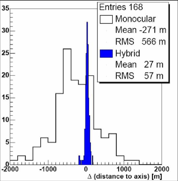
Figure 5: Resolution of the reconstructed position for vertical laser shots from the CLF.

Due to the much improved angular accuracy, the hybrid data sample is ideal for anisotropy studies. Many ground parameters, like the shower front curvature and thickness, have always been difficult to measure experimentally, and were usually determined from Monte Carlos simulation. The hybrid sample provides a unique opportunity in this respect. As mentioned, the geometrical reconstruction can be done using only one ground station, thus all the remaining detectors can be used to measure the shower characteristics. The possibility of studying the same set of air showers with two independent methods is valuable in understanding the strengths and limitations of each technique. The hybrid analysis benefits from the calorimetry of the fluorescence technique and the uniformity of the surface detector aperture [33].

We show in the Figure 6 a typical particle distribution at the ground, for a shower with an energy of 10 EeV, with a zenith angle of 45^∘. Although gammas and electrons and positrons dominate the shower, at large distances from the core and at large angles, muons come to dominate the particle distributions.

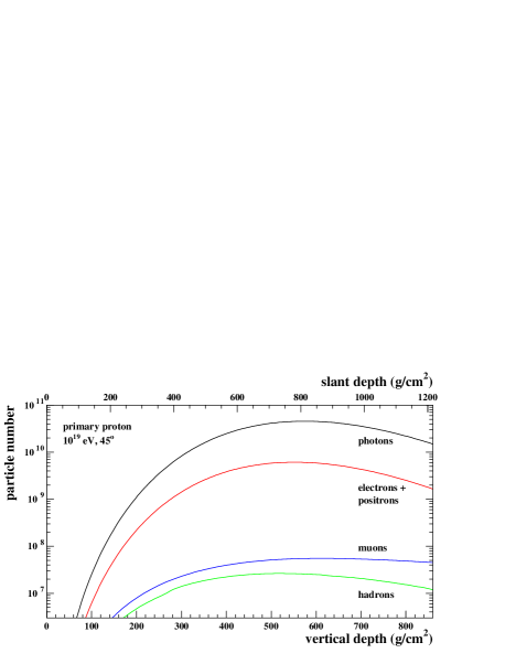
Figure 6: Particle distribution at ground from a shower of 10 EeV at an angle of 45$\circ$.

III Auger data

Since the begining of operations in 2001, Auger has been taking data continuously, first in the Engineering Array mode, which is already reported [18]. Since January 2004 it is taking data in Physics Mode, with results that will be reported in the following. A typical example of an event recorded by the SD system is shown in the Figure 7. The energy of the shower is infered from the lateral distribution function (ldf), fitted from density of particles hitting each tank at distinct distances [34, 35]. The density of particles at 1 km from the core, S(1000), is quite independent of the nature of the primary cosmic ray, according to distributions extracted from shower simulation programs, as mentioned before. Each station in the array is continuously calibrated by collecting at regular intervals signals generated by single muons. From this signal the value of a VEM (vertical equivalent muon) is extracted, taking into account variations in the atmospheric temperature and pressure.

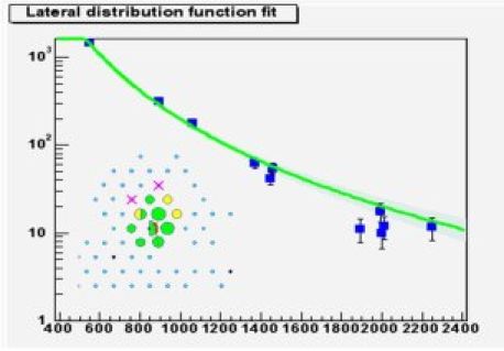
Figure 7: A typical event registered by the SD system, shown in the Event Display. The shower has a zenith angle of 30^∘ and 10 stations are used in the fitting of the lateral distribution function. The signal is quoted in VEM (Vertical Equivalent Muon).

The Auger ground stations are sensitive to very inclined showers once it has a reasonable cross-section due to the 1.2 m column of water. The very inclined showers will have transversed a larger amount of atmospheric matter before hitting the station and a large part of the electromagnetic shower will have dissipated, allowing for a much larger relative muon component. An example of this class of event is displyed in Figure 8 with a shower hitting 31 stations, coming with a zenith inclination of 88^∘.

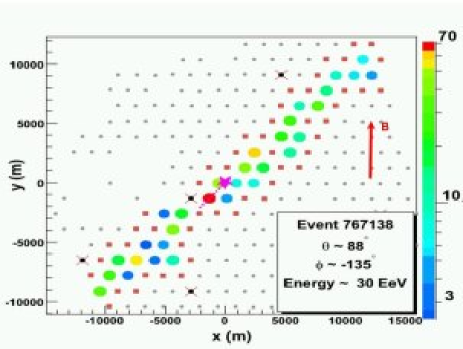
Figure 8: Event with a large zenith angle, 88^∘ in this case. Most of the signal is carried by the surviving muons, once a large part of the electromagnetic shower has been dissipated.

The structure of the FD events is exhibited in Figure 9, taken from the event monitoring system. On both pictures the map of the pixels are shown as if one would be facing the sky. So, the first event, a typical low energy shower, is flying top-down, right to left. The histogram on the top-right of the display shows the time structure of the signal in a selection of the pixels. The colour code is there just to correlate the pixel and the signal. Each bin on the right plot corresponds to 100 ns, so that the span of the signal from 260 to 360 units, actually corresponds to a time interval of 10$\mu$s. The bottom picture of Figure 9 represents a typical event propagating downwards, while the top part there is an laser shot event, with a time structure going upwards.

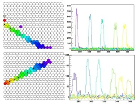
Figure 9: Typical FD events. The camera display represent the shower projected on the sky. The color code just identify the pixel. The black dots on the pixels mark those exhibited on the right. The time axis on the right side histogram is set in units of 100 ns, the label 350 means 35 $\mu$s. Top: Typical Laser shot event, where the light goes from the ground up. Lower: Regular event.

To reconstruct the geometry of the shower, first the shower detector plane (sdp) is infered by optimizing the line of light crossing the camera, using the signals as weight. The best estimate of the normal vector to the sdp, $\vec{n}_{SDP}$, is obtained by minimizing

$$\chi^{2}=\sum_{i}w_{i}[\vec{n}_{SDP}\cdot\vec{r}_{i}]^{2}$$

where the signal measured in pixel $i$ is used with the weight $w_{i}$ and the $\vec{r}_{i}$ corresponds to the direction pointing to the source in the sky. The three dimensional geometry is recovered using the angular velocity of the signal. For each shower pixel $i$ the average time of the arrival of the light at that pixel field of view, $t_{i}$, is determined from the FADC traces. The expression [36],

$$t_{i}=t_{0}+\frac{R_{p}}{c}\tan\left[\frac{(\chi_{0}-\chi_{i})}{2}\right],$$

allow for a fitting of the shower parameters, $R_{p}$, $\chi_{0}$ and $t_{0}$. Here, $c$ is the velocity of light, $R_{p}$ the shower distance of closest approach to the detector and $t_{0}$ the time at which the shower point reaches the position of closest approach. $\chi_{i}$, indicated on Figure 10, is the direction of the pixel $i$ projected onto the sdp and $\chi_{0}$ is the angle between the shower axis and the direction from the detector to the shower landing point. Figure 11 shows an example of time versus angle plot for a shower seen in stereo mode. However, this procedure is not free of ambiguities, which can be resolved with the input from the SD system. The timing information and location from a station closest to the shower landing point can be related to the time $t_{0}$,

$$t_{0}=t_{tank}-\frac{\vec{R}_{tank}\cdot\vec{S}_{shw}}{c},$$

where $\vec{R}_{tank}$ is the vector connecting the fluorescence detector to the ground station and $\vec{S}_{shw}$ is the unit vector associated to the shower propagation.

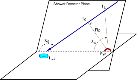
Figure 10: Shower detector plane.

To measure the energy, the light emitted by the source is reconstructed making the corrections for the atmosphere attenuation and than subtracting the Cherenkov component of the signal, identifying the fluorescence component. The time profile and the longitudinal profile for a stereo event event is exhibited in Figure 11 for both views of the event. The line fitting the longitudinal profile represents the Gaisser-Hillas function [37].

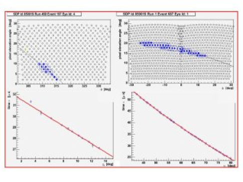
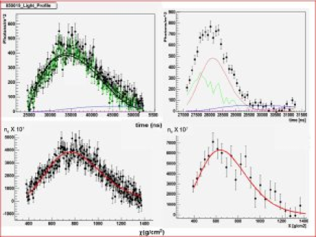
Figure 11: Event seen in stereo mode. The left hand side is the view from Los Leones and the right from Coihueco. The lower plots shows the time versus angle correlation as seen by each eye. The fit parameters are shown in the plots. Lower: The time profile and the longitudinal profile of the event above

Although there is much work to do to improve the quality of the measurements done with the SD and FD components, there are some preliminary tests that points to overall quality of the data. In particular, the correlation in the estimation of the energy of hybrid events, measured by the SD and the FD, is quite consistent.

IV Auger results

IV.1 A first estimate of the cosmic ray spectrum above 3 EeV

For the first attempt to estimate the cosmic ray spectrum above 3 EeV the analysis was based on a selection of events collected from January 1st, 2004, through June 5th, 2005. The event acceptance criteria and exposure calculation are described in a separate paper [38]. Events included in the sample have zenith angles of less than 60^∘ and energy greater than 3 EeV, resulting in a selection of 3525 events. The array is fully efficient for detecting such showers, so the acceptance at any time is given by the simple geometric aperture. The cumulative exposure adds up to 1750 km² sr yr, which is about 7% greater than the total exposure obtained by AGASA [39], along the years. The average array size during the time of this exposure was 22% of what will be available when the southern site of the Observatory has been completed.

Assigning energies to the SD event set is a two-step process, of which the first is to assign an energy parameter $S_{38}$ to each event. Then the hybrid events are used to establish the rule for converting S38 to energy. The energy parameter $S_{38}$ for each shower comes from its experimentally measured $S(1000)$, which is the time-integrated water Cherenkov signal that would be measured by a tank 1000 meters from the core.

The signal $S(1000)$ is attenuated at large slant depths. Its dependence on zenith angle is derived empirically by exploiting the nearly isotropic intensity of cosmic rays. By fixing a specific intensity $I_{0}$ (counts per unit of $\sin^{2}\theta$), one finds for each zenith angle the value of $S(1000)$ such that $I(>S(1000))=I_{0}$. We calculated a particular constant intensity cut curve CIC($\theta$) relative to the value at the median zenith angle ($\theta\approx 38^{\circ}$). Given $S(1000)$ and $\theta$ for any measured shower, the energy parameter $S_{38}$ is defined by $S_{38}\equiv S(1000)/CIC(\theta)$. It may be regarded as the $S(1000)$ measurement the shower would have produced if it had arrived 38^∘ from the zenith.

The $S_{38}$ parameter is well correlated to the energy extracted from well reconstructed hybrid showers, as can be seen at Figure 12. The fitted line gives an empirical rule for assigning energies in EeV, based on the $S_{38}$ parameter, given in VEM,

$$E=0.16\times S^{1.06}_{38}=0.16\times\left[S(1000)/CIC(\theta)\right]^{1.06}$$

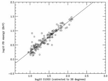
Figure 12: Shower energy for hybrid events as a function of the surface detector parameter $S_{38}$.

On the top picture of Figure 13 we show the preliminary spectrum extracted from the data up to June 2005. Plotted on the vertical axis is the differential intensity

$$\frac{dI}{d\ln E}\equiv E\frac{dI}{dE}.$$

Error bars on the points indicate the statistical uncertainty (or 95% CL upper limit). Systematic uncertainty is indicated by double arrows at two different energies. On the bottom of Figure 13, the percentage deviation from the best-fit power law, $100\times((dI/d(\ln E)-F)/F$, is shown. The fitted function is

$$F=30.9\pm 1.7\times{\rm(E/EeV)}^{-1.84\pm 0.03},$$

with a chisquare per degree of freedom of 2.4.

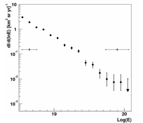
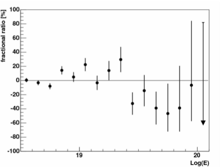
Figure 13: Top: Estimated spectrum. Lower: Deviation of the behaviour of the spectrum, in relation to a power law (see text).

V Anisotropy studies around the Galactic Center

The AGASA experiment [40, 41] and the SUGAR experiment [42] have reported an excess of cosmic rays coming from the general direction of the center of our galaxy, with energies in the EeV range. There is a very massive black hole at the center of the galaxy (CG), which provides a natural candidate for a cosmic ray accelerator to very high energies. Thus this region provides an attractive target for anisotropy studies with the Pierre Auger Observatory.

For this analysis a data set was selected comprising all the SD events collected from January 1st, 2004, until June 6th, 2005, with a zenith angle less than 60^∘. Events from the Surface Detector that passed the 3-fold or the 4-fold data acquisition triggers and satisfyed our high level physics trigger (T4) and our quality trigger (T5) [20] were selected. The T5 selection is independent of energy and ensures a better quality for the event reconstruction. This data set has an angular resolution better than 2.2^∘ [43] for all of the 3-fold events, regardless of the zenith angle considered, and better than 1.7^∘ for events with multiplicities larger than 3 SD stations.

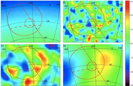
Figure 14: Lambert projections of the galactic centre region, GC (cross), galactic plane (solid line), regions of excess of AGASA and SUGAR (circles), AGASA f.o.v. limit (dashed line). The explanation of each figure is detailed in the text.

To estimate the coverage map, needed to construct excess probability maps, a shuffling technique was used. Figure 14A shows the coverage map obtained from the SD sample in a region around the GC. It has the same color scale as the significance maps, but limited to the range 0 to 1. Figures 14B, C and D, present the chance probability distributions [44] – mapped to positive Gaussian significance for excesses and negative for deficits – in the same region for various filtering and energy cuts corresponding to the various searches. Figures 14B is the significance map in the range from 0.8 to 3.2 EeV, smoothed using the individual pointing resolution of the events and a 1.5^∘ filter (Auger like excess), while 14C is the same, smoothed at 3.7^∘ (SUGAR like excess). Figure 14D covers the range from 1.0 to 2.5 EeV, smoothed at 13.3^∘ (AGASA like excess). In these maps the chance probability distributions are consistent with those expected as a result of statistical fluctuations from an isotropic sky.

In the region where the AGASA excess was reported, there are 1155 events in the energy range from 1.0 to 2.5 EeV observed at the Auger Observatory, which is to be compared to an expected sample of 1160.7 events, thus a ratio of $1.00\pm 0.03$.

These results are not compatible with the excess reported by AGASA. The level of 22% excess that they observed would translate into a $7.5\ \sigma$ excess. At the worst case scenario, where the source would be made of nucleons and the bulk of the background at this energy range made of much heavier nuclei (e.g. Iron), the difference in detection efficiency of the Auger trigger at 1 EeV would reduce the sensitivity to a source excess. However, using the ratio of Fe (70 %) to proton (50 %) efficiency at 1 EeV (1.44, an upper bound in the range from 1 to 2.5 EeV) a $5.2\ \sigma$ event excess would still be expected from our data set.

We observe in the angular/energy window, where SUGAR claims an excess, 144 events observed against 150.9 expected, with a ratio $0.95\pm 0.08$. With over an order of magnitude more statistics we are not able to confirm this claim.

A search was performed for signals of a point-like source in the direction of the galactic center using a 1.5^∘ Gaussian filter corresponding to the angular resolution of the SD [43]. In the energy range of 0.8 to 3.2 EeV, we obtain 24.3 events observed, against 23.9 expected, with a ratio $1.0\pm 0.1$. A 95% CL upper bound on the number of events coming from a point source in that window is $n_{s}=6.7$. This bound can be translated into a flux upper limit ($\Phi_{s}$) integrated in this energy range. In the simplest case in which the source has a spectrum similar to the one of the overall CR spectrum (${\rm d}N/{\rm d}E\propto E^{-3}$),

$$\Phi_{s}=n_{s}\ \Phi_{CR}\ 4\ \pi\ \sigma^{2}/n_{exp},$$

where $\sigma$ is the size of the Gaussian filter used. Using

$$\Phi_{CR}(E)=1.5\ \xi\ \left(E/EeV\right)^{-3}\times 10^{-12}\ {\rm(EeV^{-1}m^{-2}s^{-1}sr^{-1})},$$

where $\xi$, a number in the range from 1 to 2.5, denotes our uncertainty on the CR flux ($\xi$ is around unity for Auger and 2.5 for AGASA), introducing the factor $\epsilon$ for the iron/proton detection efficiency ratio ($1<\epsilon<1.6$ for E in the range from 0.8 to 3.2 EeV) and, integrating in that energy range we obtain :

$$\Phi_{s}<2.6\ \xi\ \epsilon\ \times 10^{-15}m^{-2}s^{-1}\ \ \ \ (95\%\ {\rm CL}).$$

In the worst case scenario, where both $\xi$ and $\epsilon$ take their maximum value, the bound is $\Phi_{s}=10.6\times 10^{-15}$ m^-2 s^-1, excluding the neutron source scenario, suggested by the references [41, 45], to account for the AGASA excess, or by [46, 47], in connection with the HESS measurements. More details about the GC anisotropy studies with the Auger Observatory data can be found in [48].

VI An upper limit on the primary photon fraction

The photon upper limit derived here is based on the direct observation of the longitudinal air shower profile and makes use of the hybrid detection technique and $X_{max}$ is used as discriminant observable. The information from triggered surface detectors in hybrid events considerably reduces the uncertainty in shower track geometry.

The data were taken by the 12 fluorescence telescopes at the Los Leones and Coihueco eyes, from January 2004 up to April 2005. The number of deployed surface detector stations grew from about 200 to 800 during this period. For the analysis, hybrid events were selected, i.e. showers observed both, by the surface tanks (at least one) and the telescopes [33]. Even for one triggered tank only, the additional timing constraint allows a significantly improved geometry fit to the observed profile, which leads to a reduced uncertainty in the reconstructed $X_{max}$.

The reconstruction is based on an end-to-end calibration of the fluorescence telescopes [28], on monitoring data of local atmospheric conditions [30, 49], and includes an improved subtraction of Cherenkov light [50] and reconstruction of energy deposit profiles for deriving the primary energy. In total, 16 events with energies above $10^{19}$ eV are selected. The total uncertainty $\Delta X^{tot}_{max}$ of the reconstructed depth of shower maximum is composed of several contributions which, in general, vary from event to event. A conservative estimate of the current $X_{max}$ uncertainties gives $\Delta X^{tot}_{max}\simeq 40$ g cm^-2. Among the main contributions, each one in general well below $\Delta X_{max}$ = 15 g cm^-2, are the statistical uncertainty from the profile fit, the uncertainty in shower geometry, the uncertainty in atmospheric conditions such as the air density profile, and the uncertainty in the reconstructed primary energy, which is taken as input for the primary photon simulation. For each event, high-statistics shower simulations are performed for photons for the specific event conditions. A simulation study of the detector acceptance to photons and nuclear primaries has been conducted. For the chosen cuts, the ratio of the acceptance to photon-induced showers to that of nuclear primaries (proton or iron nuclei) is $\epsilon=0.88$. A corresponding correction is applied to the derived photon limit. Figure 15 shows as an example an event of 16 EeV primary energy observed with $X_{max}$ = 780 g cm^-2, compared to the corresponding $X_{max}$ distribution expected for simulated primary photons. With $<X^{\gamma}_{max}>\ =1020$ g cm^-2, photon showers are on average expected to reach maximum at depths considerably greater than observed. Shower-to-shower fluctuations are large due to the LPM effect (rms of 80 g cm^-2) and well in excess of the measurement uncertainty. For all 16 events, the observed $X_{max}$ is well below the average value expected for photons. The $X_{max}$ distribution of the data is also displayed in Figure 15. More details about this analysis can be found in [51].

The statistical method for deriving an upper limit follows that introduced in [52]. For the Auger data sample, an upper limit on the photon fraction of 26% at a confidence level of 95% is derived. In Figure 16, this upper limit (Auger) is plotted together with previous experimental limits, from AGASA (A1) [53] , (A2) [52] and Haverah Park (HP) [54] data and compared to some estimates based on non-acceleration models (ZB, SHDM and TD from [55] and SHDM’ from [56]). The presented 26% limit confirms and improves the existing limits above 10¹⁹ eV. More details of this analysis can be found in [51] and references therein.

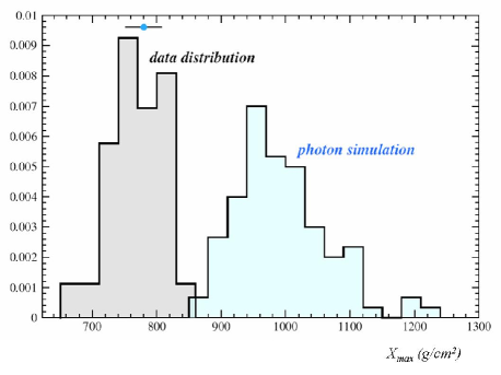
Figure 15: Example of $X_{max}$ measured in an individual shower of 16 EeV (point with error bar) compared to the $X_{max}$ distribution expected for photon showers (solid line). Also shown the $X_{max}$ distribution of the data sample (dashed line).

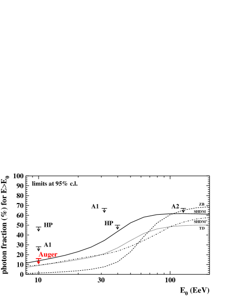
Figure 16: Upper limits on cosmic-ray photon fraction compared with previous experiments and estimates based on non-acceleration models (see main text).

VII Summary

The Pierre Auger Observatory is still under construction but has already the largest integrated exposure to high energy cosmic rays. The combination of fluorescence and the surface detector measurements allow for the reconstruction of the shower geometry and its energy with much greater quality than what could be achieved with either detector standing alone. Each of the detectors have different systematics, allowing for valuable information for cross-checking the results from each of them.

The observatory should be finished by mid 2007, accumulating by then a much larger exposure than what was used for the preliminary results presented here. That will allow for the search of anisotropies in the southern sky, as well as the test of the predicted GZK suppression.

References

- [1] M. Nagano and A. A. Watson. Rev. Mod. Phys., 72:689, 2000.
- [2] M. S. Longair. High Energy Astrophysics, Vol1: Particles, photons and their detection. Cambridge Univ. Press, Cambridge, 2 edition, 1992.
- [3] M. A. Shea and D. F. Smart. 19th international cosmic ray conference (La Jolla, USA), 4:501, 1985.
- [4] F. A. Aharonian et al. Nature, 432:75, 2004.
- [5] J. W. Cronin. Rev. Mod. Phys., 71:S165, 1999.
- [6] A. V. Olinto. Phys. Rep., 333-334:329, 2000.
- [7] J. Linsay. Phys. Rev. Lett., 10:146, 1963.
- [8] J. Linsay. Proc. 8th International Cosmic Ray Conference, 4:295, 1963.
- [9] M. A. Lawrence, R. J. O. Reid, and A. A. Watson. J. Phys. G, 17:733, 1991.
- [10] N. N. Efimov et al. Proc. Intl. Symp. on Astrophysical Aspects of the Most Energetic Cosmics Rays, page 20. eds. M. Nagano and F. Takahara, World Scientific, Singapore, 1991.
- [11] D. J. Bird et al. Phys. Rev. Lett., 71:3401, 1993.
- [12] S.Yoshida, H. Dai, C. C. H. Jui, and P. Sommers. Astrophys. J., 479:547, 1997.
- [13] M. Takeda et al. Phys. Rev. Lett., 81:1163, 1998.
- [14] K. Greisen. Phys. Rev. Lett., 16:748, 1966.
- [15] G. T. Zatsepin and V. A. Kuzmin. Sov. Phys. JETP Lett., 4:78, 1966.
- [16] The Pierre Auger Collaboration. The Pierre Auger Observatory design report. FERMILAB-PUB-96-024, 1996.
- [17] The Pierre Auger Collaboration. The Pierre Auger Observatory Technical Design Report. (http://www.auger.org/admin), 2001.
- [18] J. Abraham et al. Nucl. Instr. Meth., A 523:50, 2004.
- [19] C. Pryke. Nucl. Instr. Meth., A 354:354, 1995.
- [20] D. Allard et al. Proceedings of the 29th International Cosmic Ray Conference (Pune, India), 7:287, 2005.
- [21] M. Aglietta et al. Proceedings of the 29th International Cosmic Ray Conference (Pune, India), 7:279, 2005.
- [22] K. S. Capelle, J. W. Cronin, G. Parente, and E. Zas. Astropart. Phys., 8:321, 1998.
- [23] O. Deligny C. Lachaud X. Bertou, P. Billoir and A. Letessier-Selvon. Astropart. Phys., 17:183, 2002.
- [24] J. Bellido et al. Proceedings of the 29th International Cosmic Ray Conference (Pune, India), 7:13, 2005.
- [25] R. Sato and C. O. Escobar. Proceedings of the 29th International Cosmic Ray Conference (Pune, India), 8:13, 2005.
- [26] H. Kleifges and Auger Collaboration. Nucl. Instr. Meth., A 518:180, 2004.
- [27] C. Aramo et al. Proceedings of the 29th International Cosmic Ray Conference (Pune, India), 8:101, 2005.
- [28] P. Bauleo et al. Proceedings of the 29th International Cosmic Ray Conference (Pune, India), 8:5, 2005.
- [29] R. Mussa et al. Nucl. Instr. Meth., A 518:183, 2004.
- [30] R. Cester et al. Proceedings of the 29th International Cosmic Ray Conference (Pune, India), 8:347, 2005.
- [31] F. Arqueros et al. Proceedings of the 29th International Cosmic Ray Conference (Pune, India), 8:335, 2005.
- [32] P. Allison et al. Proceedings of the 29th International Cosmic Ray Conference (Pune, India), 8:307, 2005.
- [33] M. A. Mostafa. Proceedings of the 29th International Cosmic Ray Conference (Pune, India), 7:369, 2005.
- [34] A. M. Hillas. Proc. of the 12th ICRC, 3:1001, 1971.
- [35] Y. Matsubara M. Nagano H. Y. Dai, K. Kasahara and M. Teshima. J. Phys. G, 14:793, 1988.
- [36] P. Sommers. Astropart. Phys., 3:349, 1995.
- [37] Thomas K. Gaisser and A Hillas. Proccedings of the 15th International Cosmic Ray Conference (Plovdiv, Bulgaria), 8:353, 1977.
- [38] D. Allard et al. 2005.
- [39] N. Sakaki et al. M. Takeda. Astropart. Phys., 19:447, 2003.
- [40] M. Teshima. 26th International Cosmic Ray Conference (Salt Lake City, Utah).
- [41] N. Hayashida et al. Astropart. Phys., 10:303, 1999.
- [42] J. A. Bellido, R. W. Clay, B. R. Dawson, and M. Johnston-Hollitt. Astropart. Phys., 15:167–175, 2001.
- [43] C. Bonifazi. Proceedings of the 29th International Cosmic Ray Conference (Pune, India), 7:17, 2005.
- [44] T.-P. Li and Y.-Q. Ma. Astrophys. J., 272:317, 1983.
- [45] M. Bossa et al. J. Phys. G, 29:1409, 2003.
- [46] F. Aharonian et al. (HESS Collaboration). Astron. Astrophys., 425:L13, 2004.
- [47] F. Aharonian and A. Neronov. Astrophys. J., 619:306, 2004.
- [48] J. Abraham et al. Anisotropy studies around the galactic centre at eev energies with the auger observatory. Submited to Astropart. Phys., arXiv:astro-ph/0607382, 2006.
- [49] J. Bluemer et al. Proceedings of the 29th International Cosmic Ray Conference (Pune, India), 7:123, 2005.
- [50] F. Nerling et al. Proceedings of the 29th International Cosmic Ray Conference (Pune, India), 7:131, 2005.
- [51] J. Abraham et al. An upper limit to the photon fraction in cosmic rays above 10**19 ev from the pierre auger observatory. Submited to Astropart. Phys., arXiv:astro-ph/0606619, 2006.
- [52] M. Risse et al. Phys. Rev. Lett., 95:171102, 2005.
- [53] K. Shinozaki et al.. Astrophys. J., 571:L117, 2002.
- [54] M. Ave, J. A. Hinton, R. A. Vazquez, A. A. Watson, and E. Zas. Phys. Rev. Lett., 85:2244–2247, 2000.
- [55] G. Gelmini, O. Kalashev, and D. V. Semikoz. arXiv:astro-ph/0506128, 2005.
- [56] J. R. Ellis, V. E. Mayes, and D. V. Nanopoulos. arXiv:astro-ph/0512303, 2005.