Radial and rotational velocities of young brown dwarfs and very low-mass stars in the Upper Scorpius OB association and the $\rho$ Ophiuchi cloud core

Abstract

We present the results of a radial velocity (RV) survey of 14 brown dwarfs (BDs) and very low-mass (VLM) stars in the Upper Scorpius OB association (UScoOB) and 3 BD candidates in the $\rho$ Ophiuchi dark cloud core. We obtained high-resolution echelle spectra at the Very Large Telescope using Ultraviolet and Visual Echelle Spectrograph (UVES) at two different epochs for each object, and measured the shifts in their RVs to identify candidates for binary/multiple systems in the sample. The average time separation of the RV measurements is 21.6 d, and our survey is sensitive to the binaries with separation $<0.1$ au. We found that 4 out of 17 objects (or $24^{+16}_{-13}$ per cent by fraction) show a significant RV change in 4–33 d time scale, and are considered as binary/multiple ‘candidates.’ We found no double-lined spectroscopic binaries in our sample, based on the shape of cross-correlation curves. The RV dispersion of the objects in UScoOB is found to be very similar to that of the BD and VLM stars in Chamaeleon I (Cha I). We also found the distribution of the mean rotational velocities ($v\,\sin i$) of the UScoOB objects is similar to that of the Cha I, but the dispersion of $v\,\sin i$ is much larger than that of the Cha I objects.

1 Introduction

Most stars are member of binary systems and it is therefore important that a complete star formation theory be able to predict the binary fraction, period distribution, and mass-ratio distribution of stellar objects across a wide range of masses. Furthermore, the study of individual binary systems is the only direct means to determine fundamental stellar properties such as stellar masses and radii.

Recent high-resolution imaging studies of brown dwarfs (BDs) and very low-mass (VLM) stars have placed strong constraints on binaries with separations of $\sim 1-100\,\mathrm{au}$. For example, Hubble Space Telescope (HST) observations of $\alpha$ Per and the Pleiades indicates a binary fraction ($f$) of $>10$ per cent with a bias towards separations ($a$) of less than $15$ au, and a mass-ratio ($q$) of $>0.7$ (Martín et al., 2003) for objects around and below the hydrogen burning limit (see also Bouy et al. 2006). A similar lack of wide binaries was found in the field T-dwarf study (Burgasser et al., 2003), while $f\approx 15$ per cent (for the field objects with 0.03–0.1 $\mathrm{M_{\sun}}$ and M8.0–L0.5) was determined by Close et al. (2003) using the adaptive optics at Gemini North. They also found the vast majority of systems have a semimajor axis $<20\,\mathrm{au}$ (see also Siegler et al. 2005 but note too the results of Luhman 2004). An HST study of more than 80 field late M and L dwarfs (Gizis et al., 2003) indicated $f\approx 15$ per cent with separations in the range of 1.6–16 au. For a small (12) sample of BDs and VLM stars (0.04–0.1 $\mathrm{M_{\odot}}$) in Upper Scorpius OB association (UScoOB), Kraus, White, & Hillenbrand (2005) found $f=25_{-8}^{+16}$ per cent for $5\,\mathrm{au}<a<18\,\mathrm{au}$ by using a similar imaging technique. More recently, Basri & Reiners (2006), combined with the results of earlier works, found the upper limit of the overall binary fraction for VLM stars of $26\pm 10$ per cent.

Using a Monte Carlo simulation, the data from radial velocity surveys available in the literature, and by carefully considering the sensitivity and sampling biases, Maxted & Jeffries (2005) found an overall BD/VLM binary frequency of 32–45 per cent assuming $f=15$ per cent for $a>2.6$ au. A recent photometric study (Pinfield et al., 2003) of low-mass objects in Pleiades and Praesepe suggested, albeit indirectly, $f$ as large as 50 per cent. which would only be compatible with direct imaging studies if 70–80 per cent of those binaries have $a<1\,\mathrm{au}$. For a more comprehensive review of the current status of BD/VLM binary fraction and the separation distribution, readers are refer to a recent review of multiplicity studies by Burgasser et al. (2006).

The extensive imaging surveys provide excellent observational constraints on wider BD+BD binaries, but it is now necessary to search for shorter period BD+BD binaries systematically. Binaries with the separation of less than 1 au are not resolved by current imaging techniques, but will be detectable as spectroscopic binaries, providing the mass-ratio is not too extreme, and velocity separation is large enough. The first BD+BD spectroscopic binary, PPl 15 (Basri & Martín, 1999), showed a double-peaked cross-correlation function with a maximum velocity separation of $>70\,\mathrm{km\leavevmode\nobreak\ s^{-1}}$. The binary was found to have an eccentric orbit ($e=0.4$) with a period of $\sim 5.8\,\mathrm{d}$. Basri & Martín (1999) suggested that the formation process of substellar objects is biased towards smaller separation binaries based on the short period of PPl 15 and the lack of Pleiades BD binaries with separations $>40\,\mathrm{au}$. Note that the median separation of binaries with solar-type primaries is 30 au (Duquennoy & Mayor, 1991). Pioneering work on the RVs of BDs and VLMs are presented by Guenther & Wuchterl (2003), Kenyon et al. (2005) and Joergens (2006b) who found a several binary candidates; however, the orbital parameters and masses of binaries remains unknown because the follow-up spectroscopic monitoring is lacking or is still being undertaken. In addition to the follow-up observations, the number of BDs and VLM star binary candidates needs to be increased in order to have better statistics on short-period binary parameters.

The first BD+BD eclipsing binary (2MASS J0532184–J0546085) was discovered by Stassun, Mathieu, & Valenti (2006) from the $I$-band photometric monitoring of the system. Combining their light curves and the results from the follow-up radial velocity measurements, they were able to determined the precise orbital and physical parameters of the system. The projected semimajor axis and the period of the binary are found as $0.0398\pm 0.0010$ au and $9.779621\pm 0.000042$ d respectively.

The separation distribution of BD/VLM binaries is critical to understanding their origin. There are two main models for the formation of BDs and VLM stars: first, they have low masses because they form in low-mass, dense molecular cloud cores (e.g. Padoan & Nordlund 2002); second, BD/VLM objects have low masses because they are ejected from the dense core in which they form via dynamical interactions in multiple system, cutting off their accretion before they have reached stellar masses (Reipurth & Clarke 2001; Bate, Bonnell, & Bromm 2002a). Alternatively, there is a third model in which a free-floating BD or planetary-mass object can be formed in the process of the photo-evaporation (e.g. McCaughrean & Andersen 2002; Whitworth & Zinnecker 2004) with the outer layers of a pre-stellar core ($\sim 0.2\,\mathrm{M_{\odot}}$) removed by the strong radiation pressure from the nearby massive OB stars before the accretion onto the protostar at core centre occurs.

Due to the dynamical interaction involved in the second model, BD/VLM binaries that survive are generally expected to have small separations. In the first model, wider binaries may be expected to be more common. Bate, Bonnell, & Bromm (2002b) suggested that close binaries ($a<10\,\mathrm{au}$) do not form directly, but result from hardening of wider systems though a combination of dynamical interactions, accretion and interactions with circum-binary discs. If BD/VLM binaries have formed through such mechanisms, one would not expect to find binaries with 1–10 au separations without also finding many with separation $<1$ au. If an absence/rarity of binaries with 1 au were found, it may support the idea that they are ejected quickly from multiple systems before they have undergone the interactions that shorten their periods.

Our immediate aim is to identify spectroscopic and close BD/VLM binaries using the high-resolution echelle spectroscopy at two epochs. This experiment is sensitive to VLM binaries with separations of $<0.1$ au which corresponds to a period of $\sim 10\,\mathrm{d}$. A larger sample of candidates will enable us to measure the binary fraction of these short-period/close binaries (once confirmed), and address whether there is a significant population of ‘hidden’ VLM companions. The long term goal of this project to follow up the binary candidates found in this paper by spectroscopically monitoring them over different time scales, enabling us to obtain the radial velocity curves and their minimum masses.

In Section 2, we describe the observations and the data reduction. The results of radial velocity and rotational velocity ($v\,\sin i$) measurements are presented in Section 3. We discuss the binary/multiplicity fraction indicated by our RV survey in Section 4, and give our conclusions in Section 5.

Table 1: Summary of known properties of the targets from literature: a. Luhman & Rieke (1999) (original list for $\rho$ Oph), b. Ardila, Martín, & Basri (2000) (original list for UScoOB), c. Wilking, Greene, & Meyer (1999), d. Muzerolle et al. (2003), e. Kraus et al. (2005), and f. Mohanty, Jayawardhana, & Basri (2005).

Object	Sp.	mass	RV	$v\sin i$	Known multiple?
		$\left[\mathrm{M_{\odot}}\right]$	$\left[\mathrm{km\,s^{-1}}\right]$	$\left[\mathrm{km\,s^{-1}}\right]$
GY 5	$\mathrm{M7^{c}}$	$0.07^{\mathrm{d}}$	$-6.3\pm 1.9^{\mathrm{d}}$	$16.8\pm 2.7^{\mathrm{d}}$	no
GY 141	$\mathrm{M8.5^{a}}$	$0.02^{\mathrm{d}}$	…	$6.0^{f}$	no
GY 310	$\mathrm{M8.5^{c}}$	$0.08^{\mathrm{a,d}}$	…	$10.0^{f}$	no
USco 40	$\mathrm{M5^{b}}$	$0.1^{\mathrm{b}}$	…	$37.5^{f}$	no
USco 53	$\mathrm{M5^{b}}$	$0.1^{\mathrm{b}}$	…	$45.0^{f}$	no
USco 55	$\mathrm{M5.5^{b}}$	$0.10+0.07^{\mathrm{e}}$	…	$12.0^{f}$	$\mathrm{visual^{e}}$
USco 66	$\mathrm{M6^{b}}$	$0.07+0.07^{\mathrm{e}}$	$-4.4\pm 0.6^{\mathrm{d}}$	$27.5^{f}$	$\mathrm{visual^{e}}$
USco 67	$\mathrm{M5.5^{b}}$	$0.10^{\mathrm{e}}$	…	$18.0^{f}$	no
USco 75	$\mathrm{M6^{b}}$	$0.07^{\mathrm{e}}$	$-5.6\pm 1.1^{\mathrm{d}}$	$63.0^{f}$	no
USco 100	$\mathrm{M7^{b}}$	$0.05^{\mathrm{e}}$	$-8.9\pm 0.6^{\mathrm{d}}$	$50.0^{f}$	no
USco 101	$\mathrm{M5^{b}}$	$0.05^{\mathrm{b}}$	…	…	no
USco 104	$\mathrm{M5^{b}}$	$0.05^{\mathrm{b}}$	…	$16.0^{f}$	no
USco 109	$\mathrm{M6^{b}}$	$0.07+0.04^{\mathrm{e}}$	$-3.8\pm 0.7^{\mathrm{d}}$	$6.0^{f}$	$\mathrm{visual^{e}}$
USco 112	$\mathrm{M5.5^{b}}$	$0.1^{\mathrm{e}}$	…	$8.0^{f}$	no
USco 121	$\mathrm{M6^{b}}$	$0.02^{\mathrm{b}}$	$-38.9\pm 1.0^{\mathrm{d}}$	…	no
USco 128	$\mathrm{M7^{b}}$	$0.05^{\mathrm{e}}$	$-3.0\pm 1.6^{\mathrm{d}}$	$0.0^{f}$	no
USco 130	$\mathrm{M7.5^{e}}$	$0.04^{\mathrm{e}}$	…	$14.0^{f}$	no
USco 132	$\mathrm{M7^{b}}$	$0.05^{\mathrm{e}}$	$-8.2\pm 1.1^{\mathrm{d}}$	…	no

2 Observations

Our sample consists of 18 young, very low-mass objects: 15 objects in the Upper Scorpius OB association ($\mathrm{d\approx 145\,pc}$, de Zeeuw et al. 1999) from the list of Ardila, Martín, & Basri (2000) and 3 objects in the $\rho$ Ophiuchi cloud core ($\mathrm{d\approx 150\,pc}$, de Zeeuw et al. 1997) from Luhman & Rieke (1999). The spectral type of the objects range between M5 and M8.5, and the age $<\sim 10\,\mathrm{Myr}$ (Luhman & Rieke 1999; Ardila et al. 2000; Muzerolle et al. 2003; Kraus et al. 2005). The sample is not complete, and the selection was solely based on brightness and the observability. The basic properties of the targets based on the literature is summarised in Table 1.

We obtained high-resolution spectra with the Kueyen telescope of the Very Large Telescope (VLT–Cerro Parnal, Chile) using the UVES echelle spectrograph. The observations were carried out between 2004 April 5 and 2004 May 17 in service mode. For each object, spectra were obtained at two different epochs separated by 4–33 d. For each object on a given night, two separate spectra were obtained consecutively. This allows us to derive more reliable uncertainty estimates in the RV values of our targets (c.f. Joergens 2006b). The data were obtained using the red arm of UVES spectrograph with two mosaic CCDs (EEV + MIT/LL with 2k$\times$4k pixels). The wavelength coverage of 6708 – 10,250 Å  and the spectral resolution $R\approx 40,000$ were used. The slit width and length of 1” and 12” were used respectively with a typical seeing of 0.8”.

The data were reduced via the standard ESO pipeline procedures for UVES echelle spectra. In summary, the data were corrected for bias, interorder background, sky background, sky emission lines and cosmic ray hits. They were then flattened, optimally extracted, and finally the different orders were merged. No binning was performed to achieve high resolution required for the RV measurements. The wavelength was calibrated using the Thorium-Argon arc spectra with a typical value of the standard deviation of the dispersion solution of 5 mÅ  which corresponds to 0.2 $\mathrm{km\leavevmode\nobreak\ s^{-1}}$ at the central wavelength 8600 Å. However, the autoguiding of the telescope keeps the star at the centre of the slit with about a tenth of the FWHM ($1\,\mathrm{km\leavevmode\nobreak\ s^{-1}}$) which sets the upper limit for the systematic error in the RV measurements (Bailer-Jones, 2004). In fact, we find that any systematic error is negligible compared to the random error associated with our radial velocity measurements (see Section 3.1). A typical signal-to-noise ratio (S/N) per wavelength bin of the spectra is about 15, and the heliocentric velocity correction was applied to the final spectra.

In addition to the main targets in Table 1, we also obtained the spectra of LHS 49 (on 2004-April-17) and HD 140538 (on 2004-May-06), which are the RV template and the RV standard stars respectively. These data were obtained using the same telescope and the same instrument setup as for our main targets. The S/N of the both objects were about 60.

3 Results

3.1 Radial velocities

Table 2: Summary of the observations, the heliocentric radial velocities ($\mathrm{RV}$) from two-epoch and the average rotational velocities ($v\sin i$). The uncertainties of relative radial velocities ($\sigma_{\mathrm{RRV}}$) with respect to the template star LHS 049 and the average radial velocities ($\overline{\mathrm{RV}}$) are also given. N.B. the uncertainties listed along with the heliocentric radial velocities in column 4 and 6 include the uncertainty in the heliocentric RV of the template star, but $\sigma_{\mathrm{RRV}}$ in column 5 do not.

Object	Date	HJD-2453100	RV	$\sigma_{\mathrm{RRV}}$	$\overline{\mathrm{RV}}$	$v\sin i$
			$\left[\mathrm{km\,s^{-1}}\right]$	$\left[\mathrm{km\,s^{-1}}\right]$	$\left[\mathrm{km\,s^{-1}}\right]$	$\left[\mathrm{km\,s^{-1}}\right]$
GY 5	2004-Apr-24	20.7198440	$-6.77\pm 2.02$	1.96
	2004-May-07	33.7721938	$-6.02\pm 0.85$	0.68	$-6.39\pm 2.19$	$16.5\pm 0.6$
GY 141	2004-May-10	36.6712108	$-4.15\pm 0.63$	0.38
	2004-May-17	43.6683007	$-3.46\pm 0.66$	0.43	$-3.81\pm 0.91$	$4.4\pm 1.4$
GY 310	2004-Apr-24	20.8373504	$-5.27\pm 0.92$	0.77
	2004-May-09	35.8224052	$-8.19\pm 0.71$	0.51	$-6.73\pm 1.16$	$11.1\pm 6.0$
USco 40	2004-Apr-05	1.7661754	$-7.34\pm 0.52$	0.15
	2004-May-07	33.7620554	$-6.28\pm 0.52$	0.15	$-6.81\pm 0.74$	$34.2\pm 0.5$
USco 53	2004-Apr-04	0.9036653	$-8.27\pm 0.70$	0.50
	2004-May-02	28.7394676	$-7.22\pm 0.63$	0.39	$-7.75\pm 0.95$	$40.0\pm 0.6$
USco 55	2004-Apr-05	1.8422807	$-6.21\pm 0.50$	0.04
	2004-May-02	28.8141198	$-6.55\pm 0.50$	0.06	$-6.38\pm 0.71$	$22.9\pm 0.8$
USco 66	2004-Apr-05	1.7972634	$-7.24\pm 0.95$	0.81
	2004-May-02	28.7956003	$-8.38\pm 1.32$	1.22	$-7.81\pm 1.63$	$25.9\pm 1.2$
USco 67	2004-Apr-05	1.7188620	$-7.07\pm 0.67$	0.44
	2004-May-02	28.7113799	$-5.70\pm 0.58$	0.30	$-6.38\pm 0.88$	$18.4\pm 0.4$
USco 75	2004-Apr-04	0.8840376	$-6.80\pm 0.70$	0.50
	2004-May-07	33.6065432	$-6.16\pm 0.78$	0.60	$-6.48\pm 1.05$	$55.6\pm 3.0$
USco 100	2004-Apr-06	1.8179138	$-7.37\pm 0.67$	0.44
	2004-May-02	28.7752928	$-7.47\pm 0.62$	0.36	$-7.42\pm 0.91$	$43.7\pm 3.2$
USco 101	2004-Apr-04	0.8120734	$-3.25\pm 0.66$	0.44
	2004-May-02	28.6591660	$-5.03\pm 0.60$	0.32	$-4.14\pm 0.89$	$19.1\pm 0.3$
USco 104	2004-Apr-04	0.7850385	$-7.05\pm 0.61$	0.35
	2004-May-02	28.6349480	$-7.62\pm 0.57$	0.27	$-7.33\pm 0.83$	$16.7\pm 0.4$
USco 109	2004-Apr-05	1.7453989	$-4.72\pm 0.50$	0.07
	2004-May-07	33.6304878	$-4.70\pm 0.51$	0.09	$-4.71\pm 0.72$	$8.6\pm 1.2$
USco 112	2004-Apr-04	0.8552168	$-2.95\pm 0.50$	0.05
	2004-May-07	33.5826368	$-3.41\pm 0.51$	0.07	$-3.18\pm 0.71$	$5.8\pm 1.2$
USco 121	2004-Apr-24	20.7059408	$-40.76\pm 0.90$	0.74
	2004-May-02	28.6969641	$-42.48\pm 0.54$	0.20	$-41.62\pm 1.04$	$17.6\pm 1.3$
USco 128	2004-May-13	39.7978276	$-7.03\pm 0.51$	0.09
	2004-May-17	43.6108024	$-6.32\pm 0.51$	0.10	$-6.68\pm 0.72$	$3.6\pm 1.1$
USco 130	2004-May-09	35.7724090	$-3.92\pm 0.94$	0.80
	2004-May-13	39.8538830	$-3.90\pm 0.67$	0.45	$-3.91\pm 1.16$	$15.2\pm 1.1$
USco 132	2004-May-13	39.8268683	$-6.68\pm 0.53$	0.18
	2004-May-17	43.6391138	$-6.61\pm 0.54$	0.20	$-6.64\pm 0.76$	$9.1\pm 0.7$

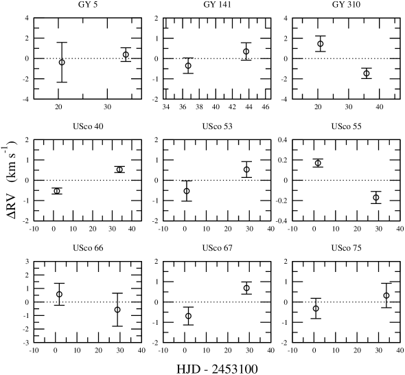
Figure 1: Relative radial velocities (RVs) of objects measured in two different epochs. The vertical axes indicate the amount of deviation ($\Delta\mathrm{RV}$) from the ‘average’ radial velocity ($\overline{\mathrm{RV}}$) in Table 2, and the horizontal axes indicate the time of the observation in heliocentric Julian date (HJD). The objects are considered to have a non-constant RV when the error bars of two data points do not overlap each other. The non-constant RV objects are considered as binary/multiple candidates.

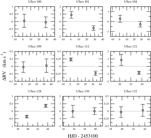
Figure 1: continued

The radial velocities of each object were determined by using the cross-correlation function of the object spectrum with that of a template star which has a similar spectra type. By visual inspection, the wavelength ranges used for the cross-correlation calculations are chosen by avoiding the regions of spectra affected by the telluric lines, and defects and fringes (in near infrared) of the CCDs. The radial velocities of objects with respect to the template are obtained by measuring the location of the peak in the cross-correlation function. The location of the peak is determined by fitting the section of the cross-correlation function around the peak by a second order polynomial. LHS 49 (Proxima Cen, M5.5) was chosen as the template for this purpose. The heliocentric radial velocity of the template object LHS 49 was obtained by measuring the wavelength shifts of the prominent photospheric absorption features K i $\lambda\lambda$7664.911, 7698.974. This gives us $\mathrm{RV_{LHS49}=}-22.6\pm 0.5\,\mathrm{km\leavevmode\nobreak\ s^{-1}}$, which is in good agreement with the earlier measurement of García-Sánchez et al. (2001) who found $\mathrm{RV_{LHS49}=}-21.7\pm 1.8\,\mathrm{km\leavevmode\nobreak\ s^{-1}}$. The heliocentric RV of each object can be then calculated by adding $\mathrm{RV_{LHS49}}$ with the RV of each object with respect to LHS 49. In the following measurements of the heliocentric radial velocities, our measurement ($\mathrm{RV_{LHS49}=}-22.6\pm 0.5\,\mathrm{km\leavevmode\nobreak\ s^{-1}}$) will be used for consistency.

Before applying the cross-correlation technique to our main targets, we have applied the technique to the radial velocity standard HD 140538 (G2.5V) for which an high-accuracy RV measurement via the fixed-configuration, cross-dispersed écelle spectrograph Elodie (Baranne & et al., 1996) is available. This was done so to ensure not only the validity of the cross-correlation technique, but also the validity of the wavelength calibration. In this test, we found the heliocentric $\mathrm{RV_{HD\,140538}=}19.17\pm 0.40\,\mathrm{km\leavevmode\nobreak\ s^{-1}}$ which is in good agreement with the Elodie radial velocity measurement of $19.00\pm 0.05\,\mathrm{km\,s^{-1}}$ (Udry, Mayor, & Queloz, 1999). Note that the uncertainty in $\mathrm{RV_{HD\,140538}}$ was computed by combining (in quadrature) the uncertainty ($0.4\leavevmode\nobreak\ \mathrm{km\leavevmode\nobreak\ s^{-1}}$) in the heliocentric RV of the template star HD 74497 (G3V) and the uncertainty in the relative RV of HD 140538 ($0.02\leavevmode\nobreak\ \mathrm{km\leavevmode\nobreak\ s^{-1}}$), measured by cross correlation with the template star. Clearly, the former dominates in the uncertainty of $\mathrm{RV_{HD\,140538}}$ shown above. The uncertainty in the heliocentric RV of the template is rather large because it was determined from a few photospheric lines.

The results of the heliocentric RV measurements (from two epochs for each object) are summarised in Table 2 along with their uncertainties. The uncertainties listed in columns 4 and 6 include the uncertainty of the absolute RV of the template star, added in quadrature with the uncertainty found from the cross correlation analysis. On the other hand, the uncertainties in the relative radial velocities ($\sigma_{\mathrm{RRV}}$) listed in column 5 of the table do not include the uncertainty of the template star. It is $\sigma_{\mathrm{RRV}}$ that is relevant for the identification of RV variable objects.

To determine the $\sigma_{\mathrm{RRV}}$, we have used the following procedure: (1) add random gaussian deviate noise to the object spectra using the corresponding variance spectra, (2) compute the cross-correlation curve using the spectra with added noise and the template, (3) measure the RV by locating the peak, (4) repeat 1–3 for 100 times, and compute the standard deviation of the 100 RV values. This should provide a good estimate of uncertainties in RVs cased by the uncertainties in the flux levels. We also estimated the RV uncertainties using the standard deviations on the mean of the two independent RV measurements obtained from the two consecutive spectra taken on the same night (c.f. Joergens 2006b). We found that these estimates agreed well with those obtained from the Monte Carlo method. The ‘average’ radial velocities $\left(\overline{\mathrm{RV}}\right)$ of the two epochs are also given in Table 2.

For each object and for each RV measurement, the deviations ($\Delta\mathrm{RV}$) from the average RV are computed and summarized in Fig. 1 along with their uncertainties ($\sigma_{\mathrm{RRV}}$) in order to aid the identification of multiplicity candidates. Note that in computing $\Delta\mathrm{RV}$ we do not require the knowledge of absolute/heliocentric radial velocities, but only the relative velocities (with respect to a template). We also cross-correlated object spectra from the two epochs (instead of using the spectra of the template LHS 49) in order to find $\Delta\mathrm{RV}$. The resulting cross-correlation functions were found to be too noisy (due to the relatively low S/N in the object spectra) for the peak positions of the cross-correlation curves to be reliably located.

To identify an object with a RV variation with a statistical significance from our sample, we apply the method described by Maxted & Jeffries (2005), which we briefly summarize next, to our data. There are three steps in this method: (1) compute the $\chi^{2}$ by fitting the two-epoch RV data for each object with a constant function (a zero-th order polynomial), (2) compute the corresponding $\chi^{2}$ probability ($p$), (3) designate the object as a non-constant RV object or a binary candidate if $p<10^{-3}$ (0.1 per cent). When computing $\chi^{2}$, we use the uncertainties in the relative RV ($\sigma_{\mathrm{RRV}}$). The number of degree of freedom in the fitting procedure is obviously 1. A similar method was also used in a recent RV survey of VLM stars by Basri & Reiners (2006).

We have computed $p$ for all the objects (Table 3), and have plotted the results as a histogram of $-\log{p}$, shown in Fig. 2 (excluding the non-member USco 121; see explanation later). The figure clearly shows two distinctive populations: one on the left (with small $-\log{p}$ values) occupied by the RV constant objects, and one on the right (with the large $-\log{p}$ values) occupied by the RV variable candidates. The expected distribution of $p$ computed consistently with our uncertainty measurements is also shown in the same figure. The RV constant population on the left side reasonably matches the expected curve. To quantify this point, we compute the $\chi^{2}$ probability to test the goodness of the fit of the expected distribution to the histogram. We restrict the fit to the first 4 bins from the left $\left(0<-\log_{10}p<2\right)$ of the histogram since the objects in the second bin from the right $\left(2.5<-\log_{10}p<3\right)$ are ‘potentially’ RV-variable, although we have flagged them as the RV-constant objects. In this analysis, we find the probability of 0.5 which indicates that the fit is reasonable. Further, if we re-normalized the expected distribution, accounting for that fact we neglected the objects in the second bin from the right, we find the $\chi^{2}$ probability of the fit increases to 0.9. This, in turn, indicates that our uncertainties in RV values are reasonable, and an additional systematic error is not necessary in this analysis. This assertion is supported by the re-analysis of BD RVs, obtained by Joergens (2006b) using the same instruments setup as ours, by Maxted & Jeffries (2005).

The boundary ($p=10^{-3}$) between the RV variable and the RV constants seems somewhat arbitrary, but here we simply adopt the definition of Maxted & Jeffries (2005). Based on this criteria, there are four objects which show significant RV variations (out of 17 samples) as one can see from the figure. They are USco 112, USco 128, USco 40, and USco 55, and considered as our preliminary binary/multiple candidates. We will discuss the binary fraction and the expected binary detection probability later in Section 4.

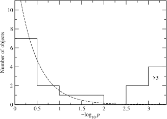
Figure 2: Histogram of the $\chi^{2}$ probability ($p$) for fitting the observed (relative) RV values with a constant (a horizontal line). The constant used in the fit is determined from the weighted mean of the two RV measurements for each object. The objects with $p<10^{-3}$ are identified as non-constant or multiple, which appear in the right-most bin in the histogram. There are four objects which satisfy this condition. The expected distribution (dashed) for RV constant objects is also shown for a comparison, and is normalized to the total number of objects that have $p>10^{-3}$. The match between the expected distribution and the histogram is reasonable (c.f. Section 3.1), indicating that our uncertainty estimates in RV values are also reasonable.

Table 3: The $\chi^{2}$ probabilities ($p$) of each object being a RV constant, listed in ascending order of $p$. The ellipses represent the boundary ($p=10^{-3}$) between RV constant objects and RV variable objects.

obj. ID	$p$
USco 112	$8.9\times 10^{-8}$
USco 128	$1.3\times 10^{-7}$
USco 40	$5.8\times 10^{-7}$
USco 55	$2.4\times 10^{-6}$
$\cdots$	$\cdots$
USco 101	$1.1\times 10^{-3}$
GY 310	$1.6\times 10^{-3}$
USco 67	$1.0\times 10^{-2}$
USco 53	$9.8\times 10^{-2}$
USco 104	$2.0\times 10^{-1}$
GY 141	$2.3\times 10^{-1}$
USco 75	$4.1\times 10^{-1}$
USco 66	$4.4\times 10^{-1}$
GY 5	$7.2\times 10^{-1}$
USco 132	$7.9\times 10^{-1}$
USco 100	$8.6\times 10^{-1}$
USco 109	$8.6\times 10^{-1}$
USco 130	$9.8\times 10^{-1}$

Finally, the histogram of $\overline{\mathrm{RV}}$ for the objects in UScoOB is given in Fig. 3. The total number of the objects is 14. Note that USco 121 is excluded from the graph since it is identified as a non-member of the UScoOB association based on the RV value (see Table 2). Muzerolle et al. (2003) also found it to be a likely non-member based on the radial velocity and the low lithium abundance. The distribution of the RVs in the figure was fitted by a gaussian function. We found that the standard deviation and the peak position of the radial velocity distribution are $1.0\,\mathrm{km\leavevmode\nobreak\ s^{-1}}$ and $-6.3\,\mathrm{km\leavevmode\nobreak\ s^{-1}}$ respectively. The former is very similar to the standard deviation (0.9 $\mathrm{km\leavevmode\nobreak\ s^{-1}}$) of the radial velocity distribution of 9 BDs and VLM objects in Cha I found by Joergens (2006a). They also studied the radial velocity distribution of more massive 25 T Tauri stars in Cha I, and found the standard deviations ($1.3\,\mathrm{km\leavevmode\nobreak\ s^{-1}}$) is not significantly different from that of the brown dwarfs and the very low-mass objects. Unfortunately, we do not have the radial velocity measurements of the higher mass counter parts (T Tauri stars) in Upper Sco OB association. This is planned for future investigation since this is important for the study of the mass dependency of the kinematics in a young stellar cluster.

According to the hydrodynamical simulations of a low-mass star-forming cluster of Bate et al. (2003) which yields a stellar density of $\sim 10^{3}\,\mathrm{stars\,pc^{-3}}$, the rms dispersion (1-D) of the stars and the BDs is $1.2\,\mathrm{km\leavevmode\nobreak\ s^{-1}}$. Similarly for the model with a higher stellar density ($\sim 10^{4}\,\mathrm{stars\,pc^{-3}}$), the rms dispersion is 2.5 $\mathrm{km\leavevmode\nobreak\ s^{-1}}$ (Bate & Bonnell 2005). The standard deviation of $\overline{\mathrm{RV}}$ ($1.0\,\mathrm{km\leavevmode\nobreak\ s^{-1}}$) found in our analysis is more comparable the lower stellar density model.

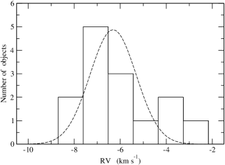
Figure 3: Histogram of the average heliocentric radial velocities of 14 UScoOB BD and VLM objects listed in Table 2 (excluding USco 121, a non-member). The gaussian fit (dashed) of the radial velocity distribution gives a standard deviation of $1.0\,\mathrm{km\leavevmode\nobreak\ s^{-1}}$ and the peak position of $-6.3\,\mathrm{km\leavevmode\nobreak\ s^{-1}}$.

3.2 Rotational velocities

The rotational velocities of the objects were determined by measuring the widths of the cross correlation functions of the target spectra against a template spectrum from an object which is known to have a very small rotational velocity. The line broadening of the targets is assumed to be dominated by rotational broadening. As in the cases for the radial velocity measurements, LHS 49 is chosen as the template. Using its rotational period ($P\approx 83\,\mathrm{d}$, Benedict & et al. 1998) and radius ($R_{*}\approx 0.145\,\mathrm{R_{\odot}}$ from the VLTI measurement by Ségransan et al. 2003), the rotational velocity of LHS 49 is estimated as $v\,\sin i=2\pi R_{*}/P\approx 0.1\,\mathrm{km\leavevmode\nobreak\ s^{-1}}$; negligibly small.

The width of the cross-correlation curves ($\sigma_{\mathrm{CCF}}$) are calibrated with the rotational velocities ($v\,\sin i$) by cross correlating the template spectra against the same template spectra with added rotation (convolved with a given $v\,\sin i$), as done by e.g. Tinney & Reid (1998), Mohanty & Basri (2003) and White & Basri (2003). A linear limb-darkening law with a solar-like parameter ($\epsilon=0.6$) was assumed in the formulation of the rotational profile described by Gray (1992), his Eq. 17.12. For each object, two measurements of rotational velocities are computed from two independent spectra obtained at different epochs. As for the RV measurements, the mean and the standard deviation of the mean are used as the final rotational velocity and its uncertainty. The final results are recorded in Table 2. In general, our measurements are in good agreement with the earlier measurements of Muzerolle et al. (2003) and Mohanty, Jayawardhana, & Basri (2005), given in Table 1. For example, Muzerolle et al. (2003) found $v\,\sin i=16.8\pm 2.7\,\mathrm{km\,s^{-1}}$ for GY 5 while we found $v\,\sin i=16.5\pm 0.6\,\mathrm{km\,s^{-1}}$.

The range of $v\,\sin i$ found among our objects is $3.6$–$55.6\,\mathrm{km\leavevmode\nobreak\ s^{-1}}$, and a similar range is also found by Mohanty et al. (2005). Fig. 4 shows the histogram of $v\,\sin i$ distribution for the UScoOB objects (14 objects excluding USco 121, non member). The log-normal fit of this distribution gives the peak position at $16.9\,\mathrm{km\leavevmode\nobreak\ s^{-1}}$ with a standard deviation $\sigma=27.8\,\mathrm{km\leavevmode\nobreak\ s^{-1}}$. Using the $v\,\sin i$ data in Joergens & Guenther (2001), the same histogram bin size used for UScoOB objects and a log-normal fit, we find the $v\,\sin i$ distribution of the BD and VLM stars (8 objects) in Cha I peaks at $15.4\,\mathrm{km\leavevmode\nobreak\ s^{-1}}$, and has the standard deviation of $8.0\,\mathrm{km\leavevmode\nobreak\ s^{-1}}$. The peak of the distribution is similar to that of Upper Sco objects, but the standard deviation of the distribution is much smaller than that of our Upper Sco objects. The difference maybe due to the very small sample. A similar fit was applied to the $v\,\sin i$ distribution of 14 higher mass T Tauri stars in Cha I using the data of Joergens & Guenther (2001), and we found a peak at $17.0\,\mathrm{km\leavevmode\nobreak\ s^{-1}}$ with a standard deviation $25.9\,\mathrm{km\leavevmode\nobreak\ s^{-1}}$ which are very similar to those of the Upper Sco brown dwarf candidates and VLM stars.

Figure 4: Histogram of the rotational velocities ($v\,\sin{i}$) of 14 UScoOB BD and VLM objects listed in Table 2 (excluding USco 121, a non-member). The log-normal fit (dashed) of the rotational velocity distribution gives a standard deviation $27.8\,\mathrm{km\leavevmode\nobreak\ s^{-1}}$ and the peak position $16.9\,\mathrm{km\leavevmode\nobreak\ s^{-1}}$.

4 Binary fraction

In Section 3.1, we found 4 out of 17 (excluding USco 121; non-member) objects show a statistically significant RV variation, indicating that they are binary/multiple candidates. In order to estimate the uncertainty in the binary/multiple fraction from this relatively small sample, we will follow the method used by Basri & Reiners (2006) who considered the binomial distribution, $P_{B}\left(x,n,p\right)$ of $x$ positive event out of $n$ trials with the probability $p$ for a positive event in each trial. In our case, $n=17$ (the number of sample) and $x=4$. The peak of $P_{B}\left(4,17,p\right)$ curve suggests the binary fraction of 24 per cent, as its should be ($4/17=0.24$). The uncertainties was estimated by plotting $P_{B}\left(4,17,p\right)$, and finding the values of $p$ at which $P_{B}$ reduced to $e^{-1}$ of the peak value. In this analysis, we find the binary/multiple fraction along with the uncertainties of our sample to be $f=24^{+16}_{-13}$ per cent.

Next, we investigate the range of semimajor axes of binaries (equivalently the range of binary periods) to which our RV survey is sensitive. For this purpose, we will consider the detection probability for binaries or the RV variables, given the time separations of two-epoch observations and the ranges of estimated primary masses (c.f. Tables 1 and 2). The probability is calculated based on the simulated RV observations of binaries whose orbit are randomly selected from a model. A similar method was used by Maxted & Jeffries (2005) and Basri & Reiners (2006). The most important factors in determining the detection probability are the size of uncertainties in RV measurements (which we use the average $\sigma_{\mathrm{RRV}}$ from our observation), and the time separations of observations. The smaller the errors in RV measurements, the larger the probability for a given binary orbit and a time separation of orbit. The larger the time separation of observations, the larger the upper limit of the semimajor axis to which an observation is sensitive. The average time separation of the two-epoch RV observations of our targets is $21.6$ d. In the following, we will briefly discuss our model assumptions and parameters which are essentially the same as those of Maxted & Jeffries (2005) but with some simplifications.

There are six basic parameters in our Monte Carlo simulation: primary mass ($M_{1}$), mass ratio ($q$), eccentricity ($e$), orbital phase ($\phi$), orbital inclination ($i$), longitude of periastron ($\lambda$). The primary mass $M_{1}$ is assigned from the adopted mass of the targets in Table 1, with a uniform random deviation of $\pm 0.002\,M_{\sun}$. The mass ratio is assumed to be uniformly distributed between $q=1.0$ and $0.2$. The eccentricity $e$ is assumed to be zero (circular orbits). Both Maxted & Jeffries (2005) and Basri & Reiners (2006) found the detection probability is insensitive to the assumed distribution of $q$ and $e$. The orbital phase is randomly chosen between 0 and 1. The inclination $i$ is randomly chosen from the cumulative distribution of $\cos{i}$. The longitude of periastron $\lambda$ is not necessary since we assumed $e=0$.

In order to compute the detection probability as a function of semimajor axis $a$, we take the following procedure: (1) for each object in our targets, we randomly select $10^{5}$ binaries using the assumption stated above for a given value of $a$, and compute the RV of the primary ($V_{1}$), (2) evolve the orbit by the time separation of the RV measurements used in the observations for this object, and take another simulated measurement of RV ($V_{2}$), (3) from $V_{1}$, $V_{2}$ and the average uncertainty in RV ($\sigma_{\mathrm{RRV}}$) from the observations, we compute the $\chi^{2}$ probability $p$, and flag the trial as a detection if $p<10^{-3}$ as done for the real data, (4) find the fraction of detections out of all random trials, (5) repeat 1–4 for the range of $a$ between $10^{-3}$ and 10 au, and (6) repeat 5 for the all targets, and find the detection probability averaged over all targets as a function of $a$.

The result of the simulation is shown in Fig. 5. The detection probability curve shown here is very similar that of Basri & Reiners (2006) for a constant time separation (20 d) case (see their Fig. 4). The probability remains fairly constant up to $a\approx 0.1\,\mathrm{au}$, and it rapidly decreases beyond $a\approx 0.3\,\mathrm{au}$. This turning point will increase if we had used larger time separations in our observation. From this figure, we find that the 80 per cent detection probability up to for binaries with $a<0.1\,\mathrm{au}$, given our time separations and the average uncertainty ($\sim 0.42\,\mathrm{km\leavevmode\nobreak\ s^{-1}}$) in the RV measurements.

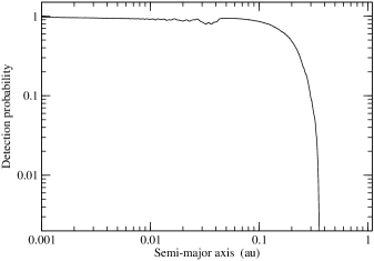
Figure 5: The binary detection probability (solid) as a function of the semimajor axis ($a$), based on Monte Carlo simulations of RV measurements, is shown. For each object in our target list, the simulation was performed using the time separation ($\Delta t$) actually used in our two-epoch observations (c.f. Table 2) and the estimated primary mass (c.f. Table 1). The final detection probability is obtained by averaging over the simulated observations of all the objects. The average time separation in the two-epoch observations is $\sim 21.6\,\mathrm{d}$, and the average uncertainty in RV is $\leavevmode\nobreak\ 0.42\,\mathrm{km\leavevmode\nobreak\ s^{-1}}$. The probability remains fairly constant up to $a\approx 0.1\,\mathrm{au}$, and it rapidly decreases beyond $a\approx 0.3\,\mathrm{au}$. The 80 per cent detection probability is achieved for binaries with $a<0.1\,\mathrm{au}$.

An alternative explanation for the RV variations found in the binary candidates above is a type of stellar pulsations found by Palla & Baraffe (2005). They studied the non-adiabatic, linear instability of very VLM stars and BD during the deuterium burning phase in the core, and found unstable fundamental modes in the time-scale between $\sim 1$ and $\sim 5$ h for the object mass from $0.02$ and $0.1\,\mathrm{M_{\odot}}$. By using their pulsation periods and by assuming that the pulsation amplitudes is 5 per cent of the radius of the objects, we find that the expected RV variation can be $>6\,\mathrm{km\leavevmode\nobreak\ s^{-1}}$. As mentioned in Section 2, for each object at a given night, two separate spectra are obtained consecutively (with time separations of $\sim 0.5$ h.). We have measured the RV from each spectrum to check if there is a large jump in the RV measurements on a short time-scale. The size of the shifts in the RV values measured in the two consecutive spectra are found in between $0.02\pm 0.10$ (USco 128) and $2.04\pm 1.67\,\mathrm{km\leavevmode\nobreak\ s^{-1}}$ (USco 66), and the average size of the shifts $0.36\,\mathrm{km\leavevmode\nobreak\ s^{-1}}$, which is much smaller than the expected RV variation based on the models of Palla & Baraffe (2005); hence, we found little indication of the pulsations in our sample.

5 Conclusions

We have presented two-epoch RV survey of 18 young BDs and VLM stars ($0.02\leavevmode\nobreak\ M_{\sun}<M_{*}<0.1\leavevmode\nobreak\ M_{\sun}$) in UScoOB and $\rho$ Oph dark cloud core using the high resolution UVES echelle spectroscopy at VLT. The average time separation of RV measurements are 21.6 d, and our RV survey is sensitive to binaries with separation smaller than 0.1 au. One of our targets, USco 121, is most likely a non-member of the UScoOB association based on the deviation of the RV from the result of the population in the association. A similar conclusion was found by Muzerolle et al. (2003) from their RV study and the low lithium abundance.

We found 4 (USco 112, USco 128, USco 40 and USco 55) out of 17 objects as our binary/multiple candidates. This corresponds to the binary fraction of $24^{+16}_{-13}$ per cent for the binary separation $a<0.1$ au. The recent high-resolution imaging survey of brown dwarfs and very low-mass objects (M5.5–M7.5 ) in the UScoOB by Kraus et al. (2005) (which was not known to authors at the time of our observation: April–May, 2004) confirms that USco 55 and USco 66 are multiple systems, and USco 109 is most likely a multiple system. Their projected separations are $a>4.0$ au which is well above our sensitivity limit of 0.1 au; therefore, it is not surprising that we did not identify USco 66 and USco 109 as multiples. Interestingly, we also found USco 55 as a candidate for a multiple system. This may indicate that it is a triple system with one of the objects located within 0.1 au of the primary. In addition, we identify USco 112 and 128 as binary candidates, but they did not find them as multiples. Further they found USco 67, 75, 130 and 132 as non-multiple, as did we.

We found the RV dispersion ($1.0\,\mathrm{km\leavevmode\nobreak\ s^{-1}}$) of the objects in UScoOB is very similar to that of the BDs and VLM stars in Chamaeleon I (Cha I) previous study by Joergens (2006a). The rotational velocities ($v\,\sin i$) of the samples were also measured. The distribution of $v\,\sin i$ for the UScoOB objects peaks around $16.9\,\mathrm{km\leavevmode\nobreak\ s^{-1}}$ which is also similar to that of the Cha I population found by Joergens (2006a); however, the dispersion of $v\,\sin i$ for the UScoOB objects ($27.8\,\mathrm{km\leavevmode\nobreak\ s^{-1}}$) is found to be much larger than that of the Cha I objects ($8.0\,\mathrm{km\leavevmode\nobreak\ s^{-1}}$)

Follow-up spectroscopic observations of the binary candidates presented here are planned in near future. There are only a few RV variable binary candidates identified in earlier surveys (Guenther & Wuchterl 2003; Kenyon et al. 2005; Joergens 2006b). As Burgasser et al. (2006) points out most of the current RV and imaging surveys use samples from magnitude-limited survey, but one should attempt to use the samples from volume-limited survey in order to find a correct statistics on binary parameters more straightforwardly, i.e. without correcting for bias. It is possible that our binary fraction is an overestimate since we are biased to brighter objects. However the lack of a double-line system suggests that a primary-to-secondary luminosity ratio of $\gg 1$ for the RV variables found in this paper.

References

- Ardila et al. (2000) Ardila D., Martín E., Basri G., 2000, AJ, 120, 479
- Bailer-Jones (2004) Bailer-Jones C. A. L., 2004, A&A, 419, 703
- Baranne & et al. (1996) Baranne A., et al., 1996, A&AS, 119, 373
- Basri & Martín (1999) Basri G., Martín E. L., 1999, AJ, 118, 2460
- Basri & Reiners (2006) Basri G., Reiners A., 2006, AJ, 132, 663
- Bate & Bonnell (2005) Bate M. R., Bonnell I. A., 2005, MNRAS, 356, 1201
- Bate et al. (2002a) Bate M. R., Bonnell I. A., Bromm V., 2002a, MNRAS, 332, L65
- Bate et al. (2002b) —, 2002b, MNRAS, 336, 705
- Bate et al. (2003) —, 2003, MNRAS, 339, 577
- Benedict & et al. (1998) Benedict G. F., et al., 1998, AJ, 116, 429
- Bouy et al. (2006) Bouy H., Moraux E., Bouvier J., Brandner W., Martín E. L., Allard F., Baraffe I., Fernández M., 2006, ApJ, 637, 1056
- Burgasser et al. (2003) Burgasser A. J., McElwain M. W., Kirkpatrick J. D., 2003, AJ, 126, 2487
- Burgasser et al. (2006) Burgasser A. J., Reid I. N., Siegler N., Close L., Allen P., Lowrance P., Gizis J., 2006, preprint (astro-ph/0602122)
- Close et al. (2003) Close L. M., Siegler N., Freed M., Biller B., 2003, ApJ, 587, 407
- de Zeeuw et al. (1997) de Zeeuw P. T., Brown A. G. A., de Bruijne J. H. J., Hoogerwerf R., Lub J., Le Poole R. S., Blaauw A., 1997, in Battrick B., ed., Proc. ESA Symp. SP-402, Hipparcos Venice ’97, ESA, Noordwijk, p. 495
- de Zeeuw et al. (1999) de Zeeuw P. T., Hoogerwerf R., de Bruijne J. H. J., Brown A. G. A., Blaauw A., 1999, AJ, 117, 354
- Duquennoy & Mayor (1991) Duquennoy A., Mayor M., 1991, A&A, 248, 485
- García-Sánchez et al. (2001) García-Sánchez J., Weissman P. R., Preston R. A., Jones D. L., Lestrade J.-F., Latham D. W., Stefanik R. P., Paredes J. M., 2001, A&A, 379, 634
- Gizis et al. (2003) Gizis J. E., Reid I. N., Knapp G. R., Liebert J., Kirkpatrick J. D., Koerner D. W., Burgasser A. J., 2003, AJ, 125, 3302
- Gray (1992) Gray D. F., 1992, The Observation and Analysis of Stellar Photospheres. Cambridge Univ. Press, Cambridge, UK
- Guenther & Wuchterl (2003) Guenther E. W., Wuchterl G., 2003, A&A, 401, 677
- Horne (1986) Horne K., 1986, PASP, 98, 609
- Joergens (2006a) Joergens V., 2006a, A&A, 448, 655
- Joergens (2006b) —, 2006b, A&A, 446, 1165
- Joergens & Guenther (2001) Joergens V., Guenther E., 2001, A&A, 379, L9
- Kenyon et al. (2005) Kenyon M. J., Jeffries R. D., Naylor T., Oliveira J. M., Maxted P. F. L., 2005, MNRAS, 356, 89
- Kraus et al. (2005) Kraus A. L., White R. J., Hillenbrand L. A., 2005, ApJ, 633, 452
- Luhman (2004) Luhman K. L., 2004, ApJ, 614, 398
- Luhman & Rieke (1999) Luhman K. L., Rieke G. H., 1999, ApJ, 525, 440
- Martín et al. (2003) Martín E. L., Barrado y Navascués D., Baraffe I., Bouy H., Dahm S., 2003, ApJ, 594, 525
- Maxted & Jeffries (2005) Maxted P. F. L., Jeffries R. D., 2005, MNRAS, 362, L45
- McCaughrean & Andersen (2002) McCaughrean M. J., Andersen M., 2002, A&A, 389, 513
- Mohanty & Basri (2003) Mohanty S., Basri G., 2003, in Brown A., Harper G. M., and Ayres T. R., eds., The Future of Cool-Star Astrophysics: 12th Cambridge Workshop on Cool Stars, Stellar Systems, and the Sun, Univ. Colorado, Boulder, 2003, p. 683
- Mohanty et al. (2005) Mohanty S., Jayawardhana R., Basri G., 2005, ApJ, 626, 498
- Muzerolle et al. (2003) Muzerolle J., Hillenbrand L., Calvet N., Briceño C., Hartmann L., 2003, ApJ, 592, 266
- Padoan & Nordlund (2002) Padoan P., Nordlund Å., 2002, ApJ, 576, 870
- Palla & Baraffe (2005) Palla F., Baraffe I., 2005, A&A, 432, L57
- Pinfield et al. (2003) Pinfield D. J., Dobbie P. D., Jameson R. F., Steele I. A., Jones H. R. A., Katsiyannis A. C., 2003, MNRAS, 342, 1241
- Reipurth & Clarke (2001) Reipurth B., Clarke C., 2001, AJ, 122, 432
- Ségransan et al. (2003) Ségransan D., Kervella P., Forveille T., Queloz D., 2003, A&A, 397, L5
- Siegler et al. (2005) Siegler N., Close L. M., Cruz K. L., Martín E. L., Reid I. N., 2005, ApJ, 621, 1023
- Stassun et al. (2006) Stassun K. G., Mathieu R. D., Valenti J. A., 2006, Nat, 440, 311
- Tinney & Reid (1998) Tinney C. G., Reid I. N., 1998, MNRAS, 301, 1031
- Udry et al. (1999) Udry S., Mayor M., Queloz D., 1999, in Hearnshaw J. B., Scarfe C. D., eds., ASP Conf. Ser. Vol. 185, IAU Colloq. 170: Precise Stellar Radial Velocities, Astron. Soc. Pac., San Francisco, p. 367
- White & Basri (2003) White R. J., Basri G., 2003, ApJ, 582, 1109
- Whitworth & Zinnecker (2004) Whitworth A. P., Zinnecker H., 2004, A&A, 427, 299
- Wilking et al. (1999) Wilking B. A., Greene T. P., Meyer M. R., 1999, AJ, 117, 469