The Zurich Extragalactic Bayesian Redshift Analyzer
(ZEBRA) and its 1^st application: COSMOS

Abstract

We present ZEBRA, the Zurich Extragalactic Bayesian Redshift Analyzer.
The current version of ZEBRA combines and extends several of the classical approaches to produce accurate photometric redshifts down to faint magnitudes. In particular, ZEBRA uses the template-fitting approach to produce Maximum Likelihood and Bayesian redshift estimates based on:
$(1.)$ An automatic iterative technique to correct the original set of galaxy templates to best represent the SEDs of real galaxies at different redshifts;
$(2.)$ A training set of spectroscopic redshifts for a small fraction of the photometric sample to improve the robustness of the photometric redshift estimates; and
$(3.)$ An iterative technique for Bayesian redshift estimates, which extracts the full two-dimensional redshift and template probability function for each galaxy.
We demonstrate the performance of ZEBRA by applying it to a sample of 866 $I_{AB}\leq 22.5$ COSMOS galaxies with available $u*$, $B$, $V$, $g^{\prime}$, $r^{\prime}$, $i^{\prime}$, $z^{\prime}$ and $K_{s}$ photometry and zCOSMOS spectroscopic redshifts in the range $0<z<1.3$. Adopting a 5-$\sigma$-clipping that excludes $\leq 10$ galaxies, both the Maximum Likelihood and Bayesian ZEBRA estimates for this sample have an accuracy $\sigma_{\Delta{}z/(1+z)}$ smaller than 0.03. Similar accuracies are recovered using mock galaxies.
ZEBRA is made available to the public at: http://www.exp-astro.phys.ethz.ch/ZEBRA.

1 Introduction

Current imaging surveys of faint high redshift galaxies such as, e.g., COSMOS (Scoville et al., 2006), already return millions of galaxies with magnitudes well beyond the current observational spectroscopic limits. As spectroscopic redshifts for such large distant galaxy samples will thus remain practically unobtainable in the foreseeable future, photometric redshifts of increasing accuracy will have to be constructed in order to properly exploit the wealth of information, as a function of cosmic epoch, that is potentially extractable from state-of-the-art and future large imaging surveys.

The importance of estimating accurate redshifts from multi-wavelength medium- and broad-band photometry for large galaxy samples is reflected in the extensive efforts that have been devoted to improving algorithms and methodologies to increase the accuracy of the photometric estimates (see, e.g., Sawicki et al. 1997; Yee 1998; Arnouts et al. 1999; Benítez 2000 (BPZ); Budavári et al. 2000; Firth et al. 2003; Benítez 2004; Brodwin et al. 2006; Ilbert et al. 2006, and references therein). These works are based on a few basic principles, namely:

$(i)$ $\chi^{2}$ minimization of the difference between a model-galaxy Spectral Energy Distribution (SED; the model SEDs are hereafter referred to as templates) and the observed galaxy photometry; $(ii)$ Neural network approaches that rely on the availability of a small sample of spectroscopic redshifts to find a functional dependence between photometric data and redshifts; $(iii)$ Hybrid approaches that perform standard $\chi^{2}$ minimization while using a small spectroscopic training sample to optimize the initial set of galaxy templates; $(iv)$ Bayesian methods which use additional information provided by a prior to obtain final photometric redshift estimates.

Motivated by the scientific returns of deriving accurate photometric redshifts for large numbers of faint COSMOS galaxies, we have developed ZEBRA, the Zurich Extragalactic Bayesian Redshift Analyzer. In this paper we describe the current version of ZEBRA, which combines and extends several of the above-mentioned approaches to produce accurate photometric redshifts down to faint magnitudes. More specifically, the paper is structured as follows:

Section 2: About ZEBRA, specifies the input requirements and the output of ZEBRA.

Section 3: The principles of ZEBRA, describes the general design and methodological details of the code. A flow chart indicating the architectural structure of ZEBRA is shown in Figure 1. Basically, ZEBRA produces two separate estimates for the photometric redshifts of individual galaxies: A Maximum Likelihood (ML) estimate, and a Bayesian (BY) estimate. These achieve a high accuracy by combining together some novel features with several of the approaches that have been published in the literature. In particular, ZEBRA:

- Uses a novel automatic iterative technique to correct an original set of galaxy templates to best represent the SEDs of real galaxies at different redshifts. These template corrections depend on the accuracies and systematic errors in the absolute photometric calibrations; therefore, prior to performing the individual template corrections, ZEBRA automatically removes systematic calibration errors in the input photometric catalogs. The template corrections substantially reduce the photometric redshift inaccuracies that are generated by galaxy-template mismatches;

- Can be fed with a training set of spectroscopic redshifts for a small fraction of the photometric sample, to improve the robustness of the photometric redshift estimates;

- Adopts an iterative technique for Bayesian photometric redshift estimates that extracts the full two-dimensional redshift and template likelihood function for each galaxy.

Section 4: The $1^{st}$ application of ZEBRA, demonstrates the performance of ZEBRA by comparing our photometric redshifts estimates for a sample of $866$ $I_{HST,AB}<22.5$ ACS-selected COSMOS galaxies with high-quality zCOSMOS spectroscopic redshifts $z_{spec}\leq 1.3$ (Lilly et al., 2006). Based on the currently available passbands and photometric accuracies, both the ML and BY ZEBRA photo-$z$’s for COSMOS galaxies have a $5\sigma-$clipped accuracy of $\Delta{}z/(1+z)=0.027$ over the entire redshift range (with $\sim 1\%$ outliers).

Section 5: Concluding remarks, briefly comments on the first applications of the COSMOS ZEBRA photometric redshifts, and lists the developments which we are already implementing in the next version of ZEBRA.

The three Appendices introduce the notation and conventions that we use throughout the paper (Appendix A), present in detail the explicit mathematical formulation of ZEBRA’s algorithms (Appendix B), and demonstrate the ZEBRA performance on a Mock catalogue produced for the COSMOS survey (courtesy of Manfred Kitzbichler; Appendix C).

ZEBRA is made available to the general public at http://www.exp-astro.phys.ethz.ch/ZEBRA.

The use of ZEBRA should please be acknowledged with an explicit reference to this paper in the bibliographic list of any resulting publication.

2 About ZEBRA

ZEBRA accepts as input:

$(i)$ A photometric catalog containing medium- and broad-band photometric data for each galaxy of the sample under study;

$(ii)$ The filter transmission curves corresponding to the passbands of the photometric catalogue, and

$(iii)$ An initial set of templates.

Optimally, photometric errors should also be included in the photometric catalog; however, it is possible to set errors to a user-specified value. Some frequently used templates and filter curves are already provided within ZEBRA.

ZEBRA offers a variety of output information depending on the program configuration:

$-$ When run in photometry-check mode (Section 3.1), the program corrects the input photometric catalog of any systematic calibration error, and returns the detailed information about the applied corrections.

$-$ In template-optimization mode (Section 3.2) ZEBRA returns the corrected templates as wavelength versus spectral-flux-density tables.

$-$ In the Maximum-Likelihood mode (section 3.3), the main output consists of the best fit redshift and template type for each galaxy in the photometric catalogue, together with their confidence limits estimated from constant $\chi^{2}$ boundaries. Additionally, the program returns: (i) the minimum $\chi^{2}$, (ii) the normalization of the best fit template, (iii) the rest-frame B-band magnitude and (iv) the luminosity distance. If specified by the user, further information is accessible, e.g. the likelihood functions for all galaxies in several output formats, and the residuals between best fit template magnitude and observed magnitude for each galaxy in each passband.

$-$ In the Bayesian mode (Section 3.4), ZEBRA calculates the 2D-prior in redshift and template space in an iterative fashion. This final prior (and, if specified, the interim prior of each iteration step) is provided, together with the posterior for each galaxy. The posterior can be saved as full 2D-table or in marginalized form. ZEBRA’s output also lists the most probable redshift and template type for each galaxy, as defined by the maximum of (i) the 2D posterior or (ii) the posterior after marginalizing over templates types and redshifts, respectively. The errors are calculated directly from the posterior.

$-$ ZEBRA can also derive and return $K$-corrections based on the specified templates and filters.

All input and output files of ZEBRA are ASCII-files.

Overall, ZEBRA is designed in a flexible way allowing all key-parameters to be user-defined. A detailed updated description of ZEBRA’s input and output, and a manual explaining its use, can be found at ZEBRA’s URL.

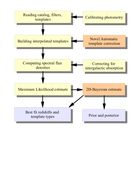
Figure 1: The architectural design of ZEBRA: the individual components are described in Section 3. The calibration of the photometric catalog and the automatic template corrections are performed by running ZEBRA in its photometry-check and template-optimization modes, respectively. In red are shown the boxes corresponding to the innovative components of ZEBRA; In particular the automatic template correction module, and the two-dimensional Bayesian module. The output of ZEBRA is indicated by blue boxes.

3 The principles of ZEBRA

3.1 Step 0: Correction of systematic calibration errors in the input photometric catalogues

In principle, with perfectly calibrated photometry, ZEBRA can be run directly in the template-optimization mode, so as to determine the optimal corrections to the original templates that allow to properly reproduce the SED of galaxies at all redshifts. If present, however, systematic calibration errors in the input photometric catalogs deteriorate the quality of the photometric redshift estimates. Such calibration errors can be easily identified, as they lead to residuals which are independent of template type between best-fit template and galaxy fluxes.

The photometry-check mode of ZEBRA offers the possibility of correcting for any such possible systematic calibration error before performing any correction to the shape of the individual templates (as done, e.g., in Benítez (2000) and Capak et al. (2004); see also Coe et al. (2006) for an application). In particular, the photometry-check mode of ZEBRA:

$-$ Computes, for each galaxy $i$ and for each filter $n$, the difference $\Delta{}\text{mag}_{n,i}$ between the magnitude of the best-fit template and the observed magnitude $\text{mag}_{n,i}$ of the galaxy in that filter.

$-$ Fits, separately for each passband but independent of the template, the dependence of the $\Delta{}\text{mag}$ residuals on the observed galaxy magnitude. A constant shift, a linear or higher order regression can be separately applied to each of the $\Delta{}\text{mag}$ vs mag relations.

$-$ Applies the derived corrections to each photometric set of data before re-iterating the procedure. The photometric corrections clearly depend on the input templates. Hence, it is important to ensure that the initial set of templates is well adapted to the galaxy types in the catalog and adequately covers the wavelength range which encompasses all passbands at all relevant redshifts. Furthermore, a photometric shift in one passband may lead to a change in the normalization of the template fits; Thus, a faster convergence of the iterative procedure can be reached by temporarily increasing the relative error in the specific passband. Tests performed by adding artifical offsets to our photometric data (observed and mock, see Section 4.1 and Appendix C) show that, with this extra step, convergence is always achieved as long as $(i)$ not all bands need significant photometric corrections (i.e. much larger than the photometric error), and $(ii)$ the passbands are not strongly correlated, e.g. they should not overlap. In Appendix C we further discuss these issues.

The main modules of ZEBRA are then run on input photometric catalogues that contain no systematic errors in the calibrations.

3.2 A key element of ZEBRA: A novel automatic template correction scheme

In principle, an advantage of template-matching approaches for photo-$z$ estimates is that they do not necessarily require a training set of galaxies with accurately known redshift from spectroscopic measurements. In practice, however, the available templates (e.g., $z=0$ galaxy SEDs or synthetic models) are typically inadequate to reproduce the SEDs of real galaxies at all redshifts. Therefore, a substantial error in the estimate of the photo-$z$’s in template-matching schemes is contributed by mismatches between real galaxies and available templates.

Budavári et al. (2000) propose, as a way to mitigate this problem, to apply the training set approach within the template-fitting method so as to optimize for the shape of the spectral template that best match the predicted galaxy colors (calculated using the spectroscopic redshift) and the observed colors. This is done by transforming the discrete template space into a linear continuous space, and using a Karhunen-Loève expansion to iteratively correct, through a $\chi^{2}$ minimization scheme, the eigenbases of a lower-dimensional subspace. As a result, spectral templates are derived that are a better match to the SEDs of the galaxies in the training set than are the initial model/empirical templates (see also Csabai et al. 2000, Budavári et al. 2001, Benítez 2004; Csabai et al. 2003 present an application of this method to SDSS data).

Given the availability of a training set of galaxies in the redshift interval of interest, ZEBRA uses a similar template correction scheme, which however extends and improves on the $\chi^{2}$-minimization approach adopted in the previous works. The improvements include:

1. The simultaneous application of the minimization scheme to all galaxies in the photometric sample at once;

2. The introduction of a regularization term in the $\chi^{2}$ expression, which prevents unphysical, oscillatory wiggles in the wavelength-dependent template correction functions;

3. A formalization of the $\chi^{2}$ minimization step that allows the use of interpolated templates (in magnitude space, so as to better sample the parameter space covered by the available original templates), and includes the effects of intergalactic absorption in a straightforward manner;

4. Template corrections optimized in different user-specified redshift regimes.

Details on the implementation of the concepts above are given in Appendix B. Briefly, ZEBRA minimizes, for all catalogue entries $i$ with best fitted template type $t$ at once, the following $\chi^{2}$ expression:

$$\chi_{t}^{2} =\frac{1}{N_{t}}\sum_{i=1}^{N_{t}}\chi_{t,i}^{2}=\sum_{k}\frac{1}{\sigma_{t,k}^{2}}(s_{t}^{\text{cor}}(k)-s_{t}^{\text{orig}}(k))^{2}$$

$$+\frac{1}{N_{t}}\sum_{i=1}^{N_{t}}\sum_{n=1}^{N_{B}}\frac{1}{\Delta_{n,i}^{2}}(f_{n,i}^{\text{cor}}-f_{n,i}^{\text{obs}})^{2}$$

$$+\sum_{k}\frac{1}{\rho_{t,k}^{2}}(s_{t}^{\text{cor}}(k+1)-s_{t}^{\text{cor}}(k)-s_{t}^{\text{orig}}(k+1)+s_{t}^{\text{orig}}(k))^{2},$$ (1)

with the following definitions:

$-$ $N_{t}$ is the set of catalogue entries, and contains all galaxies which are best fitted by template type $t$.

$-$ $\sigma_{t,k}$ is a pliantness parameter that regulates the amplitude of the deviations of the corrected template shape from the initial template shape.

$-$ $s_{t}^{\text{cor}}(k)$ is the corrected template shape for template type $t$, and is obviously a function of the wavelength $k$.

$-$ $s_{t}^{\text{orig}}(k)$ is the shape of the original template $t$.

$-$ ${\Delta_{n,i}}$ is the error of the photometric flux density in filter $n$ for galaxy $i$.

$-$ $f_{n,i}^{\text{cor}}$ is the spectral flux density of the corrected best fit template $t$ in filter band $n$ for galaxy $i$. The dependence on the best fit template type $t$, best fit redshift $z$ and template normalization $a$ is left implicit.

$-$ $f_{n,i}^{\text{obs}}$ is the observed spectral flux density of galaxy $i$ in filter band $n$.

$-$ ${\rho_{t,k}}$ is the regularization parameter, which constrains the gradients between original and corrected template shapes. The smaller $\rho$, the stronger the suppression of high-frequency oscillations in the shape of the corrected templates.

The second term in the r.h.s. of equation (3.2) minimizes the difference between observed flux $f_{n,i}^{\text{obs}}$ and template flux $f_{n,i}$ for all passbands $n$, averaged over all galaxies $i$. With the appropriate choice for the pliantness and regularization parameters, the first and third terms ensure that the correction procedure generates only templates with physically acceptable shapes. Specifically, the first term prevents too large deviations between the corrected and the uncorrected templates, and the last term regularizes the shape and inhibits strong oscillations in the SED of the corrected templates. Therefore, the minimization of the so-defined $\chi_{t}^{2}$ is a compromise between two orthogonal requirements: On the one hand, each original template is changed so that, averaging over all galaxies $i$ which are best fitted by that given original template, the corrected spectral flux density closely matches the measured spectral flux density. On the other hand, unphysical, large oscillations over small wavelength ranges are avoided when correcting the shape of the templates. The self-regulation terms maximize the stability and reliability of the template corrections , especially when only a small training and/or modest S/N data are available.

In principle, the optimal values of $\sigma$ and $\rho$ might be both template and wavelength dependent. In Figure 2 we show the effects of varying $\sigma$ and $\rho$ in the template correction procedure. In particular, a too small value for $\sigma$ inhibits template changes and thus reduces the efficacy of the corrections, and a too large value for $\sigma$ leads to unphysical high-frequency oscillations in the shape of the corrected templates. The latter effect can be avoided by choosing an appropriate value for $\rho$.

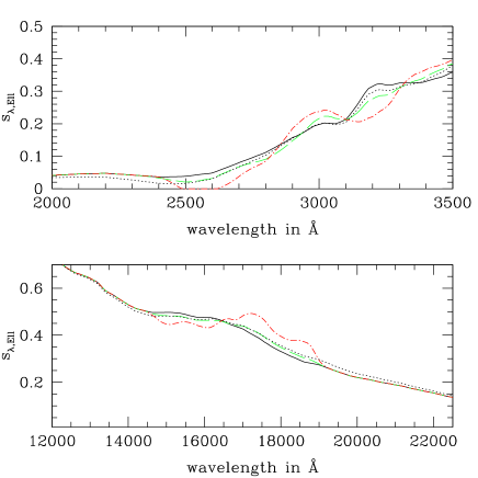
Figure 2: The figure shows the effect of varying the pliantness $\sigma$ and the regularization parameter $\rho$ on the shape of the elliptical template. Top: The original template of an elliptical galaxy (solid black line) is compared with the corrected template using the values $\sigma=2$ and $\rho=0.05$ (dotted black line). Middle and Bottom: The results of using different parameter choices are shown in detail. The solid and dotted line correspond to the same templates as above. The dashed-green ($\sigma=0.4$) and dot-dashed red ($\sigma=2$) lines result from applying the template correction scheme without regularization, i.e. setting $\rho=\infty$. The unregularized template with $\sigma=0.4$ is well-behaved, but this low value of $\sigma$ is still inadequate to properly fit the SEDs of observed galaxies. However, when choosing a five times higher pliantness ($\sigma=2$) to try to improve the correction, strong unphysical oscillations develop in wavelength ranges that are smaller than the width of the filters. The template changes are localized in separated wavelength regions and lead to unrealistic, distinguished bumps in the template shape. The high-frequency oscillations may even require to set the flux of the corrected template to zero, in order to avoid negative spectral flux densities. These unphysical “over-corrections” are avoided by choosing a finite regularization parameter $\rho$.

The ZEBRA template correction is implemented in two main steps. The procedure is started by using in step 1 only the original templates, but is iterated so that each new iteration of step 1 uses the combined set of original and corrected templates. The two main steps are:

$(1.)$ Computation of the set ${N}_{t}$ that contains all galaxies which are best fitted by the template $t$ or (from second iteration on) by a corrected template originating from template $t$.

$(2.)$ Correction of the template shape of each original template $t$ by minimizing the corresponding $\chi_{t}$ expression.

The two steps are repeated several times, as the best fit template type might change when considering new corrected templates in step 1 in the computation of ${N}_{t}$.

We note that ZEBRA can perform logarithmic interpolations of the original (and corrected) templates; thus, the $\chi^{2}$ that is actually minimized in the code is modified relative to the expression above so as to take this into account (see Appendix B for details).

Finally, ZEBRA can optimize the automatic template corrections in different redshift ranges by grouping the catalog entries in different redshift bins before the $\chi^{2}$ minimization step. This option, tested on the COSMOS data (Section 4), is found to substantially improve the reliability and quality of the ZEBRA template corrections. In Appendix C we test the method further by applying it to a mock catalog for the COSMOS survey.

3.3 The ZEBRA Maximum Likelihood module

The estimation of ML redshifts constitutes the core of the ZEBRA code. To produce the ML redshifts, ZEBRA performs the following steps (see Figure 1):

1. Read the input photometric catalog, filters and templates. The data in the catalogs (expected to be in magnitudes) are converted into spectral flux densities. Data errors are either read from the catalog or specified by the user in one of several formats.

2. Interpolate the original templates (optional). Two interpolation schemes are implemented, namely interpolation in magnitude space (“log-interpolation”) and in spectral flux density (“lin-interpolation”); these can also be used simultaneously. Specifically, a set of original templates is first sampled on a fixed wavelength grid, and then used to define the log-interpolated templates $s^{\text{log}}_{t_{1},t_{2},g}(k)$ with the weight $g$ relative to the two basic adjacent templates $s_{t_{1}}(k)$ and $s_{t_{2}}(k)$ defined as:

   $$s^{\text{log}}_{t_{1},t_{2},g}(k)=(s_{t_{1}}(k))^{1-g}(s_{t_{2}}(k))^{g},\quad{}g\in(0,1).$$ (2)

   The lin-interpolated templates $s^{\text{lin}}_{t_{1},t_{2},g}(k)$ are instead linear combinations of the basic templates:

   $$s^{\text{lin}}_{t_{1},t_{2},g}(k)=(1-g)\thinspace{}s_{t_{1}}(k)+g\thinspace{}s_{t_{2}}(k),\quad{}g\in(0,1).$$ (3)

3. Sample the filter curves on two different grids. The first grid is equal to the one used for the templates, and coarsely samples the filter shapes (as most of its elements are in wavelength bins where the transmission of the filters are equal to zero); this grid is used to optimize the speed of ZEBRA within the template correction scheme. The second grid is optimized to sample with high accuracy each individual filter in its transmission window; this high-resolution grid is used to calculate the spectral flux densities for each template in the different filter bands.

4. Correct the filter transmission functions for sharp features occurring at particular wavelengths by smoothing with a top-hat kernel. These modifications to the original filter curves are found to prevent artificial peaks in the likelihood functions; these peaks arise when e.g., a strong emission line in the galaxy or template spectrum is “trapped” in a filter-transmission “hole”, returning an overall spuriously small $\chi^{2}$ value.

5. Calculate the (redshift-optimized) corrections for each original templates as described in Section 3.2, and extend the set of available templates to include both the original and the corrected templates, and their interpolations.

6. Calculate, for each template $t$ and redshift $z$, the spectral flux densities $f_{z,t,n}$ in each filter band $n$. The mean optical depth $\tau(\lambda,z)$ of the intergalactic absorption is computed according to either Madau (1995) or Meiksin (2006) (see Appendix A). The $f_{z,t,n}$ values are stored in a three-dimensional array.

7. Determine the best fitting template normalization factor $a^{*}(z,t)$ and the value of $\chi^{2}(z,t,a^{*})$ using the formulation of Benítez (2000) (see Equation (11), Appendix A). A search in the two-dimensional array $\chi^{2}(z,t,a^{*})$ is carried out to find the minimum $\chi^{2}$ and thus the best fitting values $z^{*}$ and $t^{*}$. A pair $(z,t)$ is accepted only if the absolute $B$ magnitude $M_{B}$ lies within some (user-supplied) limits, so as to avoid mathematically good fits which are however physically unacceptable (as they would imply unrealistically dim or bright galaxies at a given redshift). Similar constraints are adopted by other authors, e.g., Rowan-Robinson (2003) adopt the range $-22.5<M_{B}<-13$.

8. Calculate the errors on the ML best fit redshift estimates using constant boundaries $\chi^{2}_{\text{min}}+\Delta{}\chi^{2}$ as (two-parameter) confidence limits. For Gaussian-distributed errors $\Delta_{n}$, the values $\Delta{}\chi^{2}$=2.3 and $\Delta{}\chi^{2}$=6.17 correspond to 1-$\sigma$ and 2-$\sigma$ confidence limits, respectively. This means that the probability that the “true” value pair $(z^{\text{true}},t^{\text{true}})$ falls in an elliptical region which extends within $[z^{*}-\Delta{}z,z^{*}+\Delta{}z]$ when projected to the $z$ axis, and within $[t^{*}-\Delta{}t,t^{*}+\Delta{}t]$ when projected to the $t$ axis, is $68.3\%$ and $95.4\%$, respectively.

The ZEBRA’s ML module computes the full likelihood functions in the two-dimensional redshift-template space, which are then used as input for the ZEBRA BY estimates.

3.4 The ZEBRA two-dimensional Bayesian module

As discussed in Benítez (2000) and Brodwin et al. (2006), employing the Bayesian method for the determination of photometric redshifts enables the inclusion of prior knowledge on the statistical properties of the galaxy sample under study, and thus to substantially improve, statistically, the accuracy of the redshift estimates.

The general idea behind Bayes theorem is that the “posterior” $P(\boldsymbol{\alpha}|\mathbf{f})$, which provides the parameters $\boldsymbol{\alpha}$ given the data $\mathbf{f}$, can be determined if the “prior” $P(\boldsymbol{\alpha})$ and the likelihood $\mathcal{L}(\boldsymbol{\alpha})$ are known. Specifically:

$$P(\boldsymbol{\alpha}|\mathbf{f})=P(\boldsymbol{\alpha})\frac{\mathcal{L}(\boldsymbol{\alpha})}{P(\mathbf{f})}.$$ (4)

Despite its name, the function $P(\boldsymbol{\alpha})$ might not be known a priori.

In Benítez (2000), the Bayesian prior is calculated by assuming an analytic function and fixing its free parameters using the available galaxy catalog. The method is powerful: an application is presented in Benítez (2004). In particular, by construction, the resulting redshift distribution is smooth and the effects of cosmic variance are reduced. The chosen analytic form may however not necessarily take properly into account the selection criteria of the galaxy catalog under study; furthermore, some assumptions on the relation amongst the different free parameters are required in order to constrain the fit.

A different approach is described in Padmanabhan et al. (2005). There, the true redshift density distribution is estimated by ”deconvolving” the measured maximum-likelihood redshift distribution from the errors of the photometric redshift estimates. This method has the advantage of being very general; however, for degenerate distributions and/or a small galaxy samples, it may not converge to a stable solution unless an additional prior is introduced.

To address these issues, Brodwin et al. (2006) propose an iterative method to build the prior self-consistently, using as a start the input photometric catalogue; in the redshift domain, this method has the advantage of closely matching specific over- and under-densities in the redshift distribution of the target field which are due to cosmic variance. These authors present extensive tests, performed on the galaxy data and using Monte Carlo simulations, to show that the method converges to a stable prior.

ZEBRA adopts the same self-consistent technique used by Brodwin et al. (2006) to derive Bayesian estimates for galaxy photometric redshifts, and furthermore extends that formulation by applying the Bayesian analysis to the full two-dimensional space of redshift and template. The equation for the prior is therefore re-written as:

$$P(z,t|\mathbf{f}_{i}^{\text{obs}})=P(z,t)\frac{\mathcal{L}_{i}(z,t)}{\sum_{z,t}P(z,t)\mathcal{L}_{i}(z,t)}.$$ (5)

Naturally, the so-constructed prior will depend on the selection criteria for the input sample. This dependence is carried over into the posterior $P(z,t|\mathbf{f}^{\text{obs}})$, which therefore represents the probability density of determining the correct $z$ and $t$, given the observed flux densities $\mathbf{f}_{i}^{\text{obs}}$ and the selection criterion for the sample. Also, note that the values $z^{*}$ and $t^{*}$ of the maximum likelihood solution, and the values $z^{\#}$ and $t^{\#}$ which maximize the posterior probability, are generally different, as the latter are weighed by the prior.

The prior is determined by starting with an user-specified guess-prior $P_{\text{old}}(z,t)$ (e.g. a flat prior; as long as the initial guess is smooth enough, the iterative prior calculation converges quickly to a unique answer; see Section 3.4.1), and calculating an improved prior $P_{\text{new}}$ as:

$$P_{\text{new}}(z,t) =P_{\text{old}}(z,t)\frac{1}{N_{G}}\sum_{i=1}^{N_{G}}\frac{\mathcal{L}_{i}(z,t)}{\sum_{z^{\prime},t^{\prime}}P_{\text{old}}(z^{\prime},t^{\prime})\mathcal{L}_{i}(z^{\prime},t^{\prime})}$$ (6)

Equation (6) follows from equation (5) by assuming that the sample is large enough to be representative, i.e.

$$\frac{1}{N_{G}}\sum_{i=1}^{N_{G}}P(z,t|\mathbf{f}_{i}^{\text{obs}})\approx{}P(z,t),$$ (7)

with $N_{G}$ the number of galaxies in the sample. By constraining the prior to remain smooth at each iterative step (by convolution with a Gaussian kernel; see below), a small number of iterations, performed by resetting, after each iteration, $P_{\text{old}}(z,t)\leftarrow{}P_{\text{new}}(z,t)$, are found to converge to a stable result for the final prior $P(z,t)$.

In practice, it is clearly advisable to exclude unreliable redshift determinations in the calculation of equation (6); these can be contributed by galaxies with poor template fits and by galaxies with too sparsely sampled SEDs (i.e., with photometric data in only a small number of passbands). In our application of ZEBRA to the COSMOS data (Section 4), we define as “good fits” those with values of $\chi^{2}$ smaller than the threshold $\chi^{2}_{\text{0.99}}$; this threshold is defined by the condition that, assuming that the $\chi^{2}$ values follow a $\chi^{2}$ distribution with $N_{filter}-3$ degrees of freedom, the probability of having a value of $\chi^{2}$ smaller than $\chi^{2}_{\text{0.99}}$ is 99%. For example, for our special application to the COSMOS data with photometry in eight filters (i.e., for five degrees of freedom), the threshold is given by $\chi^{2}_{\text{0.99}}\approx{}15$. We have tested, using as thresholds also some specified percentiles of the measured $\chi^{2}$ distribution, that the final result is rather insensitive to the choice of the threshold.

3.4.1 Smoothing of the prior

In principle, the probability density distribution of finding a galaxy at a given redshift should be a smooth function of $z$. In practice, however, $N(z)$ is estimated from the galaxy survey under study. The biased sampling of the large-scale structure, due to the finite area covered by the specific survey, and the shot-noise, due to the finite number of galaxies in the survey, generate high-frequency fluctuations in the observed redshift distribution. The presence of sharp features in the estimated number counts leads to a runaway effect in the iterative procedure to determine the best prior. For galaxies whose likelihood peaks close to the redshift of these features, the redshift estimation is fully driven by the prior. Therefore, peaks in the number counts become more and more prominent after every iteration at the expenses of the surrounding regions. The net effect is that, after a few iterations, the prior becomes very spiky.

This instability needs to be eliminated for a proper Bayesian estimation of galaxy redshifts. This can be done by building on the key ideas for introducing a prior, which are $(a)$ to account for the fact that all redshifts are not equally likely, and $(b)$ to help to distinguish between degenerate peaks of the likelihood functions. Therefore, the prior should not contain features that are narrower than the characteristic width of the peaks in the likelihood functions.

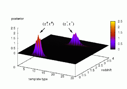
Figure 3: The two-dimensional probability distribution in template and redshift space for one of the COSMOS galaxies in the sample that we discuss in Section 4. For illustration purposes, the corrected templates used for this run of ZEBRA are collapsed in the figure onto the corresponding 31 “uncorrected” (original plus log-interpolated) templates. The values of $z^{*}$ and $t^{*}$ of the Maximum Likelihood solution, and the values $z^{\#}$ and $t^{\#}$ which maximize the posterior probability, are labeled in the figure.

A simple way to solve the problem is to smooth the prior after each iteration. The smoothing scale must be chosen by comparing a number of characteristic scales:

$(a)$ The intrinsic broadness (in redshift space) of the features originated by large-scale structures, $\sigma_{\rm LSS}$;

$(b)$ The standard error of the Maximum Likelihood estimator, $\sigma_{\rm ML}$;

$(c)$ The typical broadness of the likelihood functions, $\sigma_{\cal L}$ (which, when photometric errors are properly estimated, has to be comparable with $\sigma_{\rm ML}$); and

$(d)$ The characteristic scale of the oscillations due to finite Poisson sampling, $\sigma_{\rm P}$ (basically the maximum redshift difference between two Maximum Likelihood estimates with consecutive redshifts).

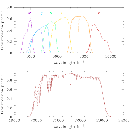
Figure 4: The transmission curves for the eight filters used to derive the COSMOS photo-$z$’s discussed in this paper. The original filters are shown as dotted lines. The adopted filter shapes are shown as solid lines. We removed “holes” in the transmission curves and smoothed them using a top-hat kernel with a FWHM of 200 Å. Top panel: the COSMOS filters $u^{*}$, $B$, $g^{\prime}$, $V$, $r^{\prime}$, $i^{\prime}$ and $z^{\prime}$. Bottom panel: The original and adopted $K_{s}$ filter shapes.

We have studied the effect of these different sources of error by performing a series of Monte Carlo simulations. In brief, we first Poisson-sample a given redshift distribution with – and without – sharp features generated by large-scale structures, and then apply our iterative procedure assuming Gaussian-shaped likelihoods. Convergence to a smooth prior is always achieved, in a few iterations, by smoothing the number counts with a Gaussian kernel of width $\sigma={\rm max}(\sigma_{\rm ML},\sigma_{\cal L},\sigma_{\rm P})$. Note that, at low-redshifts, where both $\sigma_{\rm ML}$ and $\sigma_{\cal L}$ are small, and for large samples, where also $\sigma_{\rm P}$ is small, the prior might be affected by the presence of large-scale structures. Basically all features such that $\sigma_{\rm LSS}>\sigma$ are broad enough to be robustly detected and are present in the final prior distribution. This enhances the probability of measuring redshifts close to e.g., the location of large overdensities, and leads to an optimal estimation of photometric redshift in a galaxy survey.

In ZEBRA we have thus implemented a routine to smooth the prior, at each step of the iterative procedure described above, by convolution with a Gaussian kernel with a user-specified sigma.

3.4.2 The two-dimensional probability distribution in redshift and template space

As an example, in Figure 3 we show the two-dimensional probability distribution in template and redshift space for one of the COSMOS galaxies in the sample that we discuss in Section 4. The values of $z^{*}$ and $t^{*}$ of the Maximum Likelihood solution, and the values $z^{\#}$ and $t^{\#}$ which maximize the posterior probability, are indicated in the figure. The distribution shows multiple peaks, and is dramatically different from e.g. the Gaussian shape that would be typically associated with a ML photometric redshift estimate. The key strength of the Bayesian analysis is indeed to provide, for each galaxy in a sample, such detailed information, as this is crucial to almost all statistical analyses of the evolution of galaxy properties with redshift.

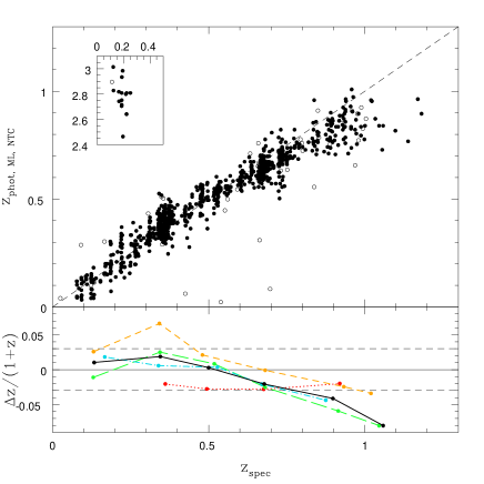
Figure 5: ML photometric redshifts for the COSMOS sample under study, derived from the uncorrected Coleman et al. (1980) and Kinney et al. (1996) templates plus their log-interpolated templates. In the upper panel, the redshift estimates $z_{\text{phot,ML,NTC}}$ are plotted against the zCOSMOS $z_{\text{spec}}$ spectroscopic redshifts. Each symbol in the plot corresponds to an individual galaxy. Empty symbols indicate a “bad” fit, defined as a fit with a reduced $\chi^{2}>$3. The lower panel shows the dependence of the accuracy of the photometric estimates, as quantified by $\Delta{}z/(1+z)$ (with $\Delta{}z=z_{\text{phot,ML,NTC}}-z_{\text{spec}}$), as a function of $z_{\text{spec}}$. Colors represent different templates: elliptical (dotted red), Sbc (short-dashed orange), Scd (long-dashed green) and irregular (dot-dashed blue) types. The total residual, independent of template type, is shown by a solid black line. Only templates which contain at least five objects in the respective redshift bin are shown. Interpolated template types are rounded to their nearest basic template type and plotted with the corresponding color. The short-dashed $\Delta{}z/(1+z)\pm{}0.03$ lines correspond roughly to 1-$\sigma$ error bars and are shown to guide the eye.

4 The $1^{st}$ application of ZEBRA: z-COSMOS-trained redshifts for COSMOS

4.1 The data, the sample and the input templates

A detailed comparison of zebra’s photo-$z$ estimates with those obtained with other codes is presented in Mobasher et al. (2006). Here we limit the demonstration of the performance of ZEBRA by using a sample of 866 $z<1.3$, $I_{AB}\leq 22.5$ COSMOS galaxies with currently available accurate (i.e., “confidence class” 3 and 4) spectroscopic redshifts from zCOSMOS (the ESO VLT spectroscopic redshift survey of the COSMOS field; Lilly et al. 2006). A further test on mock galaxies is presented in Appendix C.

These 866 galaxies with zCOSMOS spectroscopic redshifts belong to the complete sample of about $55000$ $I_{AB}\leq{}24$ COSMOS galaxies discussed in Scarlata et al. (2006); we use this complete sample to construct the initial guess-prior in the Bayesian calculation of the photometric redshifts for the COSMOS galaxies. The allowed range for the galaxy absolute $B$ magnitudes was conservatively fixed to be $-24<M_{B}<-13$.

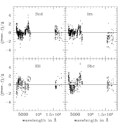
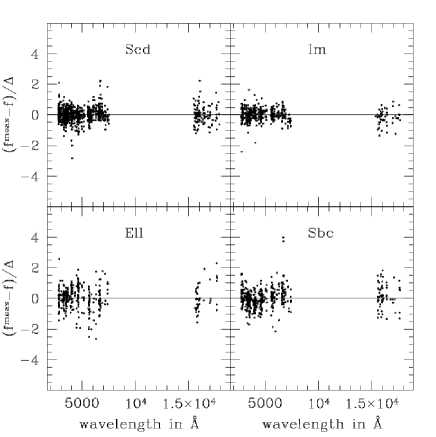
Figure 6: Error-normalized flux residuals $(f_{n,i}^{\text{obs}}-f_{n,i})/\Delta_{n,i}$ versus rest-frame wavelength for 269 galaxies with spectroscopic redshifts in the range $0.2\leq{}z<0.4$. The different panels correspond to different templates: elliptical (“Ell”) types, Sbc types, Scd types and irregular (“Im”) template types. Top: Residuals before the ZEBRA’s automatic template correction is applied. Bottom: Residuals after ZEBRA’s template correction. The systematic trends and scatter are substantially reduced.

Exploiting the wealth of ancillary data that are available for the entire COSMOS field, we use, as input photometric catalogues, Subaru $B$, $V$, $g^{\prime}$, $r^{\prime}$, $i^{\prime}$ and $z^{\prime}$ photometry ($5\sigma$ magnitude limit of $\sim$27 for point sources in all bands; Taniguchi et al. 2006); CFHT $u^{*}$ photometry ($5\sigma$ magnitude limits for point sources of $u^{*}=27.4$); and $K_{s}$ photometry from the NOAO wide–field IR imager Flamingos (Kitt Peak 4m telescope) and the Cerro Tololo ISPI (Blanco 4m telescope; all data are collected in the catalogue presented by Capak et al. 2006). About 97.2% of our spectroscopic sample has photometry available in all eight passbands. The relevant filter transmission curves are shown in Figure 4, before and after the correction for sharp features at specific wavelengths. Systematic calibration errors in each passband were estimated and corrected using the photometry-check module of ZEBRA. These were typically very small, constant shifts. The robustness of the corrections was tested by deriving them also after fixing the redshift to the spectroscopic value in the galaxy-template fits.

The adopted “original” set of templates consists of the six templates described in Benítez (2000) (which are available on the BPZ website). These are based on six observed galaxy spectra, i.e., the four of Coleman et al. (1980), i.e., an elliptical, a Sbc, a Scd and an irregular type template, and the two starbursting galaxy spectra of Kinney et al. (1996). Sawicki et al. (1997), Benítez et al. (1999) and Yahata et al. (2000) discuss and demonstrate the improvements in the quality of the redshift estimates that are obtained by augmenting the set of templates to include the starbursting types. As discussed by these previous authors, these observed templates are extended into the UV by means of a linear extrapolation up to the Lyman-Break, and into the IR (up to $\sim$ 25000Å) using GISSEL synthetic templates. We furthermore performed a 5-step log-interpolation to sample more densely the SED space covered by the original templates. This results in a basic set of 31 input (“uncorrected”) templates.

4.2 Results

To illustrate the importance of the ZEBRA template correction, we first present the comparison between the ML photometric redshifts derived when no template correction is performed ($z_{\text{phot,ML,NTC}}$), and the zCOSMOS spectroscopic redshifts ($z_{\text{spec}}$). Figure 5 presents this comparison.

In the figure, the bottom panel shows the deviation $\Delta{}z/(1+z)$ versus $z_{\text{spec}}$ (with $\Delta{}z=z_{\text{phot,ML,NTC}}-z_{\text{spec}}$), color-coded for the different templates types. Although over the entire $0\leq{}z_{\text{spec}}<1.3$ range the overall redshift estimate is acceptable (a $5-\sigma$-clipped $\sigma_{\Delta{}z/(1+z)}=0.043$ with 19 clipped galaxies), the individual templates show large systematic deviations. The elliptical and Sbc templates in particular show a significant systematic under- and overestimation of the redshifts, respectively. Furthermore, no available “uncorrected” (i.e., original plus log-interpolated) template appears to be adequate to reproduce the SEDs of $z>0.8$ galaxies: these high redshifts are systematically underestimated when using the available z=0 galaxy templates. While it remains to establish whether this systematic failure at $z>0.8$ is due to the uncertainties in the templates or to astrophysical reasons (e.g., much stronger emission lines at high redshifts than at $z=0$, or a young, passively evolving elliptical galaxy population; etc), it is clear that this systematic effect would have a substantial impact on the reliability of statistical studies of galaxy evolution with redshift.

The template correction substantially improves the photometric redshift estimates, and in particular cures the most troublesome systematic failures of the estimates derived without template correction. As an example, for galaxies with redshifts in the range $0.2\leq{}z<0.4$, Figure 6 shows the residuals $\Delta{}f$ between observed flux density and best-fit template flux density, as a function of rest-frame wavelength, before and after template corrections (using $\sigma=2$ and $\rho=0.05$). The substantial improvement in the redshift estimates is observable in Figure 7, which shows the same comparison with the zCOSMOS spectroscopic redshifts as above, but this time for the ZEBRA photometric redshift estimates with template correction ($z=z_{\text{phot,ML,TC}}$). The template corrections were optimized in the redshift bins $z$=0-0.2; 0.2-0.4; 0.4-0.6; 0.6-0.8; 0.8-1.0; 1.0-1.3 and 0-0.3; 0.3-0.5; 0.5-0.7; 0.7-0.9; 0.9-1.3). Note that the $z_{\text{phot,ML,TC}}$ redshifts at and above $\sim 0.8$ lie now well within the statistical errors. The global accuracy of the ZEBRA ML redshift estimates $z_{\text{phot,ML,TC}}$ is now reduced to a 5-$\sigma$-clipped $\sigma_{\Delta{}z/(1+z)}=0.027$ (with a clipping of only 10 galaxies).

Similar results are found when comparing the ZEBRA BY redshifts with the zCOSMOS spectroscopic redshifts. In Figure 8 we show the results of the iterative calculation of the prior using the $>56000$ galaxies in the entire ACS-selected $I_{AB}\leq 24$ COSMOS sample of Scarlata et al. (2006) from which our spectroscopic sample was extracted. The prior was obtained using an adaptive Gaussian smoothing kernel of $\Gamma=0.05(1+z)$, which was tested to lead to a stable prior estimate. In the figure, the left panel shows the prior estimate, marginalized to redshift space, after one (dotted lines) and five (solid lines) iterations. Although we only present the prior marginalized over template types, the full 2D-prior is being used for the subsequent calculation of the posterior. The right panel shows the ratio $\eta(z)$ of the marginalized priors $P(z)$, from two successive iterations: the dotted lines correspond to ratio of the priors after the second and first iteration; the solid lines show the prior ratio between the fifth and fourth iterations.

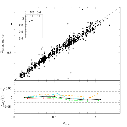
Figure 7: ZEBRA’s ML redshift estimates for the spectroscopic sample derived after correcting the templates as described in Sections 3.2 and 4. The displayed quantities are the same as in Fig. 5. The systematic trend that is visible in Fig. 5, i.e. the underestimation of the redshifts for $z\geq 0.8$, is here eliminated by the use of adequately corrected templates.

Figure 8: The marginalized prior derived from the COSMOS sample of Scarlata et al. (2006), from which our spectroscopic sample is extracted, and its convergence properties. Upper panel: The marginalized prior after the first iteration (dotted line) and after five iterations (solid line) for a Gaussian smoothing length $\Gamma=0.05(1+z)$ in redshift space. Lower panel: The point-by-point ratio of two successive redshift-marginalized prior estimations. The dotted line shows the ratio of the prior estimates between the second and first iteration. The solid line shows the prior ratio between the fifth and fourth iteration.

In Figure 9 we present the ZEBRA-zCOSMOS comparison as above, this time for the ZEBRA BY redshift estimates derived with template correction ($z_{\text{phot,BY,TC}}$). These ZEBRA BY redshifts are obtained using the values $z^{\#}$ and $t^{\#}$ which maximize the posterior. The figure highlights a similar high quality for the ML and BY ZEBRA estimates with template correction; indeed, the differences between the template-corrected BY and ML redshift estimates are vanishingly small. Of course, in BY mode ZEBRA returns the redshift and template probability distribution for each galaxy. The BY run gives a 5-$\sigma$ clipped accuracy of $\sigma_{\Delta{}z/(1+z)}=0.027$ with only 7 outliers clipped, comparable to the one derived for the ML estimates.

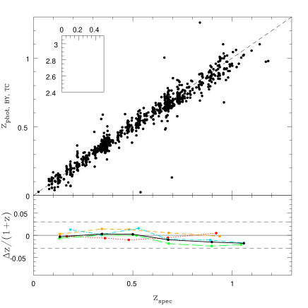
Figure 9: The application of ZEBRA’s two-dimensional Bayesian method (i) after smoothing of the projected $P(z)$ prior with a smoothing scale of $\Gamma=0.05(1+z)$ and (ii) using the same template correction as in Fig. 7. Symbols are as in Figure  5 (except that no $\chi^{2}$ threshold is shown). Similar to the ZEBRA ML estimates with template correction, also the ZEBRA BY photo-z’s with template correction eliminate the systematic trends that are present in the redshift estimates without template correction.

5 Concluding Remarks

A more thorough comparison of the ZEBRA ML and BY photo-$z$’s with the currently available zCOSMOS redshifts is given by Lilly et al. (2006). Furthermore, the ZEBRA ML and BY photometric redshift estimates are compared by Mobasher et al. (2006) with photo-$z$ estimates derived for the same galaxies with independent codes (these are either public codes, e.g. BPZ or have been developed by other teams within the COSMOS collaboration).

The ZEBRA ML photometric redshifts estimates for the COSMOS sample studied in this paper have already been used to derive the evolution up to $z\sim 1$ of the luminosity functions for morphologically-classified early-, disk- and irregular-type galaxies (according to the classification scheme of ZEST, the Zurich Estimator of Structural Types; Scarlata et al. 2006), to study the evolution up to similar redshifts of the number density of intermediate-size and large disk galaxies (Sargent et al., 2006) and to study the evolution of the luminosity function of elliptical galaxy progenitors (Scarlata et al., 2006a).

The current version (1.0) of ZEBRA is being packaged with a user-friendly web-interface at the URL provided in the abstract. The ZEBRA website will be constantly updated to provide the newest improved versions of the ZEBRA code, and the associated documentation describing in detail the implemented changes. In the meanwhile, ZEBRA is being upgraded with several new modules, including $(1)$ A module that incorporates dust absorption and reddening, according to several user-specifiable extinction corrections; $(2)$ An improved treatment of AGN’s; and $(3)$ A module that uses several synthetic template models and a large choice of self-consistent star formation and metal enrichment schemes to estimate stellar masses, average ages and metallicities (and their uncertainties).

Appendix A Notation and definitions

The filter-averaged spectral flux density of a template can be decomposed into a template-based spectral flux density $f_{z,t,n}$ and a template normalization $a$ by setting:

$$af_{z,t,n}=\frac{\int{}\frac{\mathrm{d}\nu}{\nu}\thinspace{}s^{\text{obs}}_{\nu,t}(\nu)\thinspace{}n(\nu)}{\int{}\frac{\mathrm{d}\nu}{\nu}\thinspace{}n(\nu)}$$ (8)

The spectral flux density $s^{\text{obs}}_{\nu,t}$ measured in the observer frame is related to the rest-frame template shape $s_{\nu,t}$ by:

$$s^{\text{obs}}_{\nu,t}(\nu/(1+z))=(1+z)\frac{L_{\nu}(\nu)}{4\pi{}D_{L}^{2}}=(1+z)s_{\nu,t}(\nu)a_{t}.$$ (9)

The normalization factor $a_{t}$ matches the template shape $s_{\nu,t}(\nu)$ with the apparent spectral flux density in the rest frame of a point-source with luminosity $L_{\nu}(\nu)$ at a luminosity distance $D_{L}$. The relation $a=a_{t}/(c(1+z))$ between $a$ and $a_{t}$ can then be derived from the above definitions.

For high redshift sources, attenuation effects of intervening intergalactic material, especially neutral hydrogen, become increasingly important. These attenuation effects are mostly contributed by Lyman series line-blanking and photoelectric absorption. These effects are accounted for by including a factor of $e^{-\tau(\lambda,z)}$ in the expression for $f_{z,t,n}$, i.e., defining:

$$f_{z,t,n}=\frac{\int{}\mathrm{d}\lambda\lambda\thinspace{}s_{\lambda,t}(\lambda/(1+z))\thinspace{}e^{-\tau(\lambda,z)}\thinspace{}n(\lambda)}{\int{}\mathrm{d}\lambda/\lambda\thinspace{}n(\lambda)}.$$ (10)

The ZEBRA user can choose to adopt either the Madau (1995) or the Meiksin (2006) calculation for the attenuation term; compared with the former, the latter provides a somewhat lower absorption strength at any redshift. The K-correction $K_{nl}$ between filter band $l$ in the the rest-frame and filter band $n$ in the observed-frame is defined as:

$$K_{nl}=m_{n}-M_{l}-5\log_{10}\left(D_{L}/10pc\right)$$

with $M_{l}$ the absolute magnitude in the filter $l$, and $m_{n}$ the apparent magnitude in the filter band $n$. The $K$-correction can be written as:

$$K_{nl}(z,t) =\operatorname{mag}(af_{z,t,n})-\operatorname{mag}(f^{\text{em}}_{t,l})$$

$$=\operatorname{mag}(af_{z,t,n})-\operatorname{mag}(a(1+z)f_{0,t,l})$$

$$=2.5\log_{10}(1+z)+\operatorname{mag}(f_{z,t,n})-\operatorname{mag}(f_{0,t,l}).$$

where $f^{\text{em}}_{t,n}$ is the restframe spectral flux density in the filter band $n$ and $\operatorname{mag}(x)=-2.5\log_{10}(x)$. ZEBRA can provide the $K$-corrections for all (original, interpolated and corrected) used templates.

The normalized likelihood $\mathcal{L}(z,t,a)$ can be written as:

$$\mathcal{L}(z,t,a) =\frac{P(\mathbf{f}^{\text{obs}}|z,t,a)}{\sum_{t^{\prime}}\int\mathrm{d}{}z^{\prime}\int{}\mathrm{d}{}a^{\prime}P(\mathbf{f}^{\text{obs}}|z^{\prime},t^{\prime},a^{\prime})}$$

$$=\frac{e^{-\frac{1}{2}\chi^{2}(z,t,a)}}{\sum_{t^{\prime}}\int\mathrm{d}{}z^{\prime}\int{}\mathrm{d}{}a^{\prime}e^{-\frac{1}{2}\chi^{2}(z^{\prime},t^{\prime},a^{\prime})}}$$

with $P(\mathbf{f}|\boldsymbol{\alpha})$ as the conditional probability distribution of reproducing the data $\mathbf{f}$ given the parameters $\boldsymbol{\alpha}$.

The $\chi^{2}(z,t,a)$ can be expressed as (Benítez, 2000):

$$\chi^{2}(z,t,a)=F_{OO}-\frac{F_{OT}^{2}}{F_{TT}}+\left[a-\frac{F_{OT}}{F_{TT}}\right]^{2}F_{TT}$$ (11)

where

$$F_{OO} =\sum_{n=1}^{N_{B}}\left(\frac{f_{n}^{\text{obs}}}{\Delta_{n}}\right)^{2},$$

$$F_{TT} =\sum_{n=1}^{N_{B}}\left(\frac{f_{z,t,n}}{\Delta_{n}}\right)^{2},$$

$$F_{OT} =\sum_{n=1}^{N_{B}}\frac{f_{n}^{\text{obs}}\thinspace{}f_{z,t,n}}{(\Delta_{n})^{2}}.$$

In this formulation, the best fitting template normalization $a^{*}$ is given by $a^{*}=F_{OT}/F_{TT}$. The best fitting redshift $z^{*}$ and template type $t^{*}$ follow from the maximum of $F_{OT}^{2}/F_{TT}$. The largest likelihood corresponds to the minimum $\chi^{2}_{\text{min}}=F_{OO}-(F_{OT}^{2}/F_{TT})(z^{*},t^{*})$.

Appendix B The ZEBRA $\chi^{2}$-minimization approach to template correction

We first describe the simple case when only the original set of templates is used as input, without interpolations between the original templates. We indicate with $N_{t}$ the number of catalog entries which are best fitted by a template type $t$. In Budavári et al. (2000) the spectral distribution $s_{t}^{\text{orig}}(k)$ of the original template type $t$ is changed by a $\chi^{2}$-minimization over all template shapes $s_{t}^{\text{cor}}(k)$, iteratively for all entries $i\in{}{N}_{t}$. Specifically, Budavári et al. (2000) perform the template correction by minimizing the following $\chi^{2}$ function:

$$\chi_{t,i}^{2}=\sum_{k}\frac{1}{\sigma_{t,k}^{2}}(s_{t}^{\text{cor}}(k)-s_{t}^{\text{orig}}(k))^{2}+\sum_{n=1}^{N_{B}}\frac{1}{\Delta_{n,i}^{2}}(f_{n,i}^{\text{cor}}-f_{n,i}^{\text{obs}})^{2}$$

In our approach, the shape $s_{t}^{\text{orig}}(t)$ of a given basic template $t$ is changed in one step, taking all entries $i\in{}{N}_{t}$ into account at once; furthermore, a regularization term is included in the definition of $\chi^{2}$, to avoid unphysical high frequency fluctuation in the correction of the template as a function of wavelength. We therefore determine the optimal template corrections by minimizing:

$$\chi_{t}^{2} =\frac{1}{N_{t}}\sum_{i=1}^{N_{t}}\chi_{t,i}^{2}=\sum_{k}\frac{1}{\sigma_{t,k}^{2}}(s_{t}^{\text{cor}}(k)-s_{t}^{\text{orig}}(k))^{2}$$

$$+\frac{1}{N_{t}}\sum_{i=1}^{N_{t}}\sum_{n=1}^{N_{B}}\frac{1}{\Delta_{n,i}^{2}}(f_{n,i}^{\text{cor}}-f_{n,i}^{\text{obs}})^{2}$$

$$+\sum_{k}\frac{1}{\rho_{t,k}^{2}}(s_{t}^{\text{cor}}(k+1)-s_{t}^{\text{cor}}(k)-s_{t}^{\text{orig}}(k+1)+s_{t}^{\text{orig}}(k))^{2}$$ (12)

with the variables as described in Section 3.2.

The spectral flux density $f_{n,i}^{\text{cor}}$ of the corrected template in the filter band $n$ depends on the catalog entry $i$ through its best fitted template type $t$, redshift $z$ and normalization factor $a$. Specifically:

$$f_{n,i}^{\text{cor}}=\sum_{k}T_{n}^{i}(k)s_{t}^{\text{cor}}(k),$$ (13)

where $T_{n}^{i}(k)s_{t}^{\text{cor}}(k)$ has yet to be determined.

In the Maximum Likelihood procedure (Section 3.3), the template-based spectral flux density $f_{t,z,n}$ is calculated for each template $t$, filter $n$ and redshift $z$, modulo an overall normalization constant $a$. The procedure assigns to each entry $i$ a triple $(t(i),z(i),a(i))$ so that the $\chi^{2}$ is minimized.

ZEBRA uses a linear approximation to describe the spectral flux density through the best fit template shape, i.e.:

$$f_{n,i} =a(i)f_{z(i),t(i),n}\approx{}\sum_{k}T_{n}^{i}(k)s_{t(i)}(k),\text{ with}$$

$$T_{n}^{i}(k) =\frac{(1+z(i))^{2}\thinspace{}a(i)}{\int{}\mathrm{d}\lambda{}/\lambda{}\thinspace{}n(\lambda)}\Delta\lambda\lambda_{k}\thinspace{}n(\lambda_{k}(1+z(i)))$$

The effect of intergalactic absorption is included easily by extending the definition of $T_{n}^{i}(k)$ using (10):

$$T_{n}^{i}(k)=\frac{(1+z(i))^{2}\thinspace{}a(i)}{\int{}\mathrm{d}\lambda{}/\lambda{}\thinspace{}n(\lambda)}\Delta\lambda\lambda_{k}\thinspace{}n(\lambda_{k}(1+z(i)))\thinspace{}e^{-\tau(\lambda_{k}(1+z(i)),z(i))}$$

The two-step iterative template correction then proceeds as described in Section 3.2.

When log-interpolated templates are used we define the set $\mathcal{N}_{t}$ as the set of catalog entries $i$, so that $t$ is the nearest basic type of the best fitting type $t(i)$. If $t(i)$ is a basic template, then $t=t(i)$; if $t(i)$ is an interpolated template, then $t=t_{1}$ if $g<0.5$, or otherwise $t=t_{2}$, see (2). To simplify the notation we define:

$$s^{\text{log}}_{t,g}=\begin{cases}s^{\text{log}}_{t,t^{+},g}&\text{ if }g<0.5\\ s^{\text{log}}_{t^{-},t,g}&\text{ if }g\geq{}0.5\text{.}\end{cases}$$

Here $t^{+}$ and $t^{-}$ indicate the successor and predecessor basic template of the basic template type $t$ with respect to the (assumed) global ordering.

When using interpolated templates, equation (13) has to be re-defined. In particular, a change in the shape $s^{\text{orig}}_{t}(k)$ leading to $s^{\text{cor}}_{t}(k)$ is reflected in a changed spectral flux density $f_{n,i}^{\text{cor}}$ for each entry $i\in{}\mathcal{N}_{t}$. For $g(i)<0.5$, we obtain:

$$f_{n,i}^{\text{cor}} =\sum_{k}T_{n}^{i}(k)s^{\text{log}}_{t(i),g(i)}$$

$$=\sum_{k}T_{n}^{i}(k)(s^{\text{cor}}_{t}(k))^{1-g(i)}(s_{t^{+}}(k))^{g(i)}$$

Using:

$$(s^{\text{cor}}_{t}(k))^{1-g(i)}=(s^{\text{orig}}_{t}(k))^{1-g(i)}\left(1+\frac{\xi_{t}(k)}{s^{\text{orig}}_{t}(k)}\right)^{1-g(i)}$$

and assuming that $\xi_{t}(k)=s^{\text{cor}}_{t}(k)-s^{\text{orig}}_{t}(k)$ is small in comparison with $s^{\text{orig}}_{t}(k)$, the following approximation holds:

$$f_{n,i}^{\text{cor}}\approx{}\sum_{k}T_{n}^{i}(k)(s_{t^{+}}(k))^{g(i)}(s^{\text{orig}}_{t}(k))^{1-g(i)}\left(1+(1-g(i))\frac{\xi_{t}(k)}{s^{\text{orig}}_{t}(k)}\right)$$ (14)

Similarly, for $g(i)\geq{}0.5$, we obtain:

$$f_{n,i}^{\text{cor}}\approx{}\sum_{k}T_{n}^{i}(k)(s_{t^{-}}(k))^{1-g(i)}(s^{\text{orig}}_{t}(k))^{g(i)}\left(1+g(i)\frac{\xi_{t}(k)}{s^{\text{orig}}_{t}(k)}\right)$$ (15)

In this approximation the spectral flux density depends linearly on $\xi_{t}(k)$ and $s^{\text{cor}}_{t}(k)$, respectively. With the definition $s^{\text{log}}_{t,0}=s^{\text{log}}_{t,1}=s^{\text{cor}}_{t}(k)$, the equations (14) and (15) also describe the change in spectral flux density if the best fit template is an original template.

To minimize the $\chi^{2}$, the templates are sampled on a grid linearly spaced in units of $\log(\lambda)$; all templates are normalized to the spectral flux density of unity in the B-band, in order to be able to use for each template the same pliantness $\sigma$. With the definitions:

$$g_{n}^{i} =\begin{cases}f_{n,i}^{\text{obs}}-\sum_{k}T_{n}^{i}(k)(s_{t^{+}}(k))^{g(i)}(s^{\text{orig}}_{t}(k))^{1-g(i)}&\text{ if }g(i)<0.5\\ f_{n,i}^{\text{obs}}-\sum_{k}T_{n}^{i}(k)(s_{t^{-}}(k))^{1-g(i)}(s^{\text{orig}}_{t}(k))^{g(i)}&\text{ if }g(i)\geq{}0.5\end{cases}$$

$$c_{n}^{i}(k) =\begin{cases}T_{n}^{i}(k)(s_{t^{+}}(k))^{g(i)}(s^{\text{orig}}_{t}(k))^{-g(i)}(1-g(i))&\text{ if }g(i)<0.5\\ T_{n}^{i}(k)(s_{t^{-}}(k))^{1-g(i)}(s^{\text{orig}}_{t}(k))^{g(i)-1}g(i)&\text{ if }g(i)\geq{}0.5\end{cases}$$

equation (B) can be written as:

$$\chi_{t}^{2} =\sum_{k}\frac{1}{\sigma_{t,k}^{2}}(\xi_{t}(k))^{2}+\sum_{k}\frac{1}{\rho_{t,k}^{2}}(\xi_{t}(k+1)-\xi_{t}(k))^{2}$$

$$\phantom{=}+\frac{1}{N_{t}}\sum_{i=1}^{N_{t}}\sum_{n=1}^{N_{B}}\frac{1}{\Delta_{n,i}^{2}}(g_{n}^{i}-\sum_{k}c_{n}^{i}(k)\thinspace{}\xi_{t}(k))^{2}$$ (16)

Postulating $\frac{\partial}{\partial{}\xi_{t}(l)}\chi_{t}^{2}=0$ leads to a system of linear equations in $\xi_{t}(k)$, i.e.:

$$\sum_{k}M_{t}(l,k)\thinspace{}\xi_{t}(k)=\nu_{t}(l),$$

where

$$M_{t}(l,k) =\frac{\delta_{l,k}}{\sigma_{t,k}}+\frac{1}{N_{t}}\sum_{i=1}^{N_{t}}\sum_{n=1}^{N_{B}}\frac{1}{\Delta_{n,i}^{2}}(c_{n}^{i}(k)\thinspace{}c_{n}^{i}(l))$$

$$\phantom{=}+\frac{1}{\rho_{t,k-1}}(\delta_{l,k}-\delta_{l,k-1})+\frac{1}{\rho_{t,k}}(\delta_{l,k}-\delta_{l,k+1})$$ (17)

$$\nu_{t}(l) =\frac{1}{N_{t}}\sum_{i=1}^{N_{t}}\sum_{n=1}^{N_{B}}\frac{1}{\Delta_{n,i}^{2}}(c_{n}^{i}(l)\thinspace{}g_{n}^{i})$$ (18)

The density of the $\lambda$-grid used to sample the templates determines the size of the set of linear equations. In the application to the COSMOS sample described in Section 4, we have used a grid in $\log(\lambda)$-space of about 800 points.

Attention has to be paid in carefully choosing the free parameters, in order to obtain physically meaningful corrections to the templates when using also interpolated templates. Specifically, if the absolute change $|\xi_{t}(k)|$ of a template is larger than the value $s^{\text{orig}}_{t}(k)$ of the original template at that wavelength, the approximative treatment of the log-interpolated templates becomes inappropriate. This can happen if a too high pliantness $\sigma_{t,k}$ is used, and/or if too few galaxies are available to constrain the fits that are performed to correct the templates. If a corrections would make the flux of a template negative in some wavelength region, the flux is set to zero. If that happens, the $c_{n}^{i}(k)$ coefficient is also set to zero, thereby inhibiting any further change in that template at that specific wavelength.

Appendix C Testing ZEBRA on a mock sample

We further demonstrate the performance of ZEBRA using a mock catalog that has been produced for the COSMOS field. Simulations of galaxies rely on population synthesis and dust models which may not perfectly match the observed SEDs of real galaxies. We find indeed that the use of the galaxy templates discussed in Section 4.1 provides slightly less accurate photometric redshift estimates for the mock galaxies than for real data. On the other hand, adopting the same models that were used to construct the mock galaxies when recovering their photo-$z$’s results in unrealistically accurate results. Testing the code on a mock catalog has however several advantages, as the mock catalog provides a large set of data with known precise redshifts, and hence allows us to test the reliability and stability of the code using disjoint samples for the training set (that is used for the template correction) and for the assessment of the photo-$z$ accuracy.

The mock catalog used for our tests contains about 50000 galaxies with $I\leq 22.5$ and data in five photometric bands ($B$, $g$, $i$, $r$, $K_{s}$). We used the same templates discussed in Section 4.1. In order to directly compare the results obtained with the mock data with those obtained using the zCOSMOS spectroscopic redshifts, we limited the training set to 1000 mock galaxies, and we used a sample of 10000 mock galaxies, disjoint from the training set, to perform the tests.

A run of ZEBRA in photometry-check mode on the original mock data showed that systematic photometric offsets were smaller than the assumed relative photometric error of 0.05 magnitudes. To test the effect of systematic photometric offsets, we therefore added shifts up to 0.2 mag to the mock data. These offsets were correctly identified and removed by the ZEBRA’s photometry-check mode.

ZEBRA was then run in the template-optimization mode; this was done using, for the training set, photometric data both corrected and not corrected for the added ”extra” offsets discussed above, so to establish the impact of systematic photometric errors on the template correction procedure. The entire set of original plus corrected templates was then used in the analysis.

In Table 1 we summarize the results of applying the Maximum-Likelihood mode of ZEBRA both to recover the redshifts of the training set galaxies themselves, and to estimate the redshifts of the independent set of 10000 galaxies in the ”evaluation” catalog.

Four configurations were explored, i.e., using: $(a)$ Catalog not corrected for photometric offsets and original (“uncorrected”) templates; $(b)$ Catalog corrected for systematic photometric errors and again original, uncorrected templates; $(c)$ Catalog not corrected for photometric offsets and corrected/optimized templates; (d) Catalog corrected for systematic photometric errors and corrected/optimized templates. In Figure 10 we compare the resulting photometric redshifts for the 10000 galaxy “evaluation sample”.

Catalog	Phot.	Templ.	$\sigma$	$\Delta{}z/(1+z)$	$\%$
	corr.	optim.
Training	no	no	0.1008	-0.051	1.3
Training	yes	no	0.0526	-0.001	2.7
Training	no	yes	0.0785	-0.029	0.7
Training	yes	yes	0.0345	0.000	1.0
Evaluation	no	no	0.1004	-0.050	1.2
Evaluation	yes	no	0.0590	-0.001	2.4
Evaluation	no	yes	0.0780	-0.029	0.5
Evaluation	yes	yes	0.0350	-0.001	1.4

Table 1: Results of the application of ZEBRA in Maximum-Likelihood mode to 1000 mock galaxies that are also used as training set (“Training” catalog), and of the application of the code to a sample of 10000 mock galaxies (“Evaluation” catalog) not overlapping with the “Training” catalog. The second column indicates whether the photometric catalogs are corrected for systematic errors; the third column indicates whether the template-correction scheme has been applied. Columns four and five list the accuracy $\sigma_{\Delta{}z/(1+z)}$ and the mean offset $\Delta{}z/(1+z)$ of the photometric redshift when compared with the “true” redshifts after 5-$\sigma$ clipping. The percentage of 5-$\sigma$ outliers is listed in the last column. Note the high accuracy and lack of global shift that is obtained when both the corrections to the photometric catalogs and the template optimization are applied; also, accuracies of the same order are obtained in the “Training” and “Evaluation” runs.

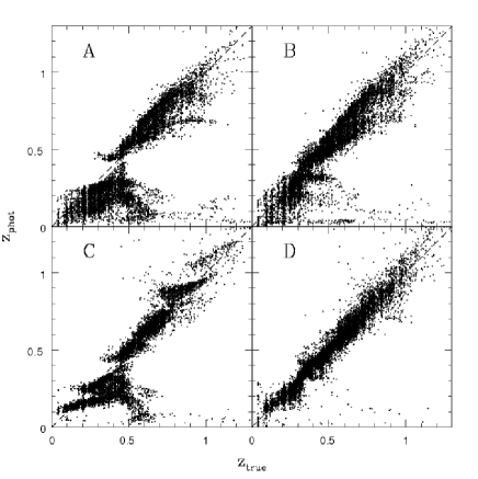
Figure 10: The comparison between the ZEBRA photometric redshifts and the “true” redshifts of the mock galaxies. The figure refers to the “evaluation” runs in which 1000 galaxies are used as the training set, and the evaluation of the performance is made on a non-overlapping sample of 10000 mock galaxies. Four different cases are shown: (a) The catalogs contains substantial photometric offsets, and the templates are not optimized; (b) The photometry correction scheme is now applied, but no template optimization has yet been performed; (c) No photometric correction is performed, but the template optimization scheme has been applied; (d) Photometric errors are removed from both the evaluation sample and the training sample, and the template optimization scheme is applied.

These tests indicate that:

1. The accuracies of the photometric redshifts obtained when applying ZEBRA to the galaxies of the training sample itself and to the disjoint evaluation sample are nearly identical (see Table 1). This shows that results of the photometry-check mode and template-optimization mode are robust and lead to a high accuracy in the redshift estimates;

2. Systematic photometric errors may indeed lead to substantial systematic artefacts in the photometric redshift estimates, which need to be removed before the template correction is performed;

3. Accurate redshifts without significant systematic artefacts can only be achieved if both photometric corrections and template corrections are employed.

References

- Arnouts et al. (1999) Arnouts S., Crisitiani S., Moscardini L., Matarrese S., Lucchin F., Fontana A., Giallongo E., 1999, MNRAS, 310, 540
- Benítez et al. (1999) Benítez N., Broadhurst T., Bouwens R., Silk J., Rosati P., 1999, ApJ, 515, L65
- Benítez (2000) Benítez N., 2000, ApJ, 536, 571
- Benítez (2004) Benítez N. et al., 2004, ApJS, 150, 1
- Brodwin et al. (2006) Brodwin M., Lilly S. J., Porciani C., McCracken H. J., Le Fèvre O., Foucaud S., Crampton D., Mellier Y., 2006, ApJS, 162, 20
- Budavári et al. (2000) Budavári T., Szalay A. S., Connolly A. J., Csabai I., Dickinson M., 2000, AJ, 120, 1588
- Budavári et al. (2001) Budavári T., et al. 2001, AJ, 122, 1163
- Capak et al. (2004) Capak P. et al., 2004, AJ, 127, 180
- Capak et al. (2006) Capak P. et al., 2006, ApJS, COSMOS Special Issue
- Coe et al. (2006) Coe D., Benítez N., Sanchez S. F., Jee M., Bouwens R., Ford H., 2006, ArXiv Astrophysics e-prints, arXiv:astro-ph/0605262
- Coleman et al. (1980) Coleman G. D., Wu C.-C., Weedman D. W., 1980, ApJS, 43, 393
- Csabai et al. (2000) Csabai I., Connolly A. J., Szalay A. S., & Budavári T., 2000, AJ, 119, 69
- Csabai et al. (2003) Csabai I. et al., 2003, AJ, 125, 580
- Efstathiou et al. (1991) Efstathiou G., Bernstein G., Tyson J. A., Katz N., Guhathakurta P., 1991, ApJ, 380, L47
- Fernández-Soto et al. (2002) Fernández-Soto A., Lanzetta K. M., Chen H.-W., Levine B., Yahata N., 2002, MNRAS, 330, 889
- Firth et al. (2003) Firth A. E., Lahav O., Somerville R. S., 2003, MNRAS, 339, 1195
- Ilbert et al. (2006) Ilbert O. et al., 2006, AA, in press, arXiv:astro-ph/0603217
- Kinney et al. (1996) Kinney A. L., Calzetti D., Bohlin R. C., McQuade K., Storchi-Bergmann T., Schmitt H. R., 1996, ApJ, 467, 38
- Lilly et al. (2006) Lilly S. J. et al., 2006, ApJS, COSMOS Special Issue
- Madau (1995) Madau P., 1995, ApJ, 441, 18
- Meiksin (2006) Meiksin A., 2006, MNRAS, 365, 807
- Mobasher et al. (2006) Mobasher B. et al., 2006, ApJS, COSMOS Special Issue
- Padmanabhan et al. (2005) Padmanabhan N. et al., 2005, MNRAS, 359, 237
- Rowan-Robinson (2003) Rowan-Robinson M., 2003, MNRAS, 345, 819
- Sargent et al. (2006) Sargent M. T. et al., 2006, ApJS, COSMOS Special Issue,
- Sawicki et al. (1997) Sawicki M. J., Lin H., Yee H. K. C., 1997, AJ, 113, 1
- Scarlata et al. (2006) Scarlata C. et al., 2006, ApJS, COSMOS Special Issue
- Scarlata et al. (2006a) Scarlata C. et al., 2006a, ApJS, COSMOS Special Issue
- Scoville et al. (2006) Scoville N. et al., 2006, ApJS, COSMOS Special Issue
- Taniguchi et al. (2006) Taniguchi Y. et al., 2006, ApJS, COSMOS Special Issue
- Yahata et al. (2000) Yahata N., Lanzetta K. M., Fernandez-Soto A., Pascarelle S. M., Chen H.-W., 2000, Bulletin of the American Astronomical Society, 32, 1602
- Yee (1998) Yee H. K. C., 1998, ArXiv Astrophysics e-prints, arXiv:astro-ph/9809347