Synthetic properties of bright metal-poor variables. I. “Anomalous” Cepheids.

We present new grids of evolutionary models for the so-colled “Anomalous” Cepheids (ACs), adopting $Z$=0.0001 and various assumptions on the progenitor mass and mass-loss efficiency. These computations are combined with the results of our previous set of pulsation models and used to build synthetic populations of the predicted pulsators as well as to provide a Mass-Luminosity relation in the absence of mass-loss. We investigate the effect of mass-loss on the predicted boundaries of the instability strip and we find that the only significant dependence occurs in the Period-Magnitude plane, where the synthetic distribution of the pulsators is, on average, brighter by about 0.1 mag than the one in absence of mass-loss. Tight Period-Magnitude relations are derived in the $K$ band for both fundamental and first overtone pulsators, providing a useful tool for distance evaluations with an intrinsic uncertainty of about 0.15 mag, which decreases to $\sim$ 0.04 mag if the mass term is taken into account. The constraints provided by the evolutionary models are used to derive evolutionary (i.e, mass-independent) Period-Magnitude-Color relations which provide distance determinations with a formal uncertainty of the order of $\sim$ 0.1 mag, once the intrinsic colors are well known. We also use model computations from the literature to investigate the effect of metal content both on the instability strip and on the evolutionary Period-Magnitude-Color relations. Finally, we compare our theoretical predictions with observed variables and we confirm that a secure identification of actual ACs requires the simultaneous information on period, magnitude and color, that also provide constraints on the pulsation mode.

1 Introduction

While the majority of metal-poor radial pulsating variables is represented by the RR Lyrae stars, other classes of variables are observed in metal-poor stellar systems. According to the current literature, one finds the “Anomalous” Cepheids (AC) and the “Population II” Cepheids (P2C), the former with periods ($P$) from $\sim$ 0.5 to $\sim$ 2 days, the latter from $\sim$ 1 to 25 days. Both types of variables are brighter than RR Lyrae stars and belong to the central He-burning evolutionary phase, as are RR Lyrae stars. However. ACs are more massive whereas P2Cs are less massive than RR Lyrae stars with similar metal content. The purpose of the present paper is to perform a theoretical analysis of the ACs, which are observed in the majority of the Local Group dwarf galaxies which have been surveyed for variable stars, but that are almost absent in other metal-poor stellar systems such as Galactic Globular Clusters. The origin of this “anomaly” is the evidence that they do not follow the Period-Luminosity relation of the P2Cs observed in these old metal deficient clusters, being significantly brighter at fixed period (see Norris & Zinn 1975; Zinn & Searle 1976; Smith & Stryker 1986; Nemec et al. 1994).

Several authors (Dolphin et al. 2002, 2003; Clementini et al. 2003; Cordier, Goupil & Lebreton 2003) have suggested that ACs are the natural extension of the Population I Classical Cepheids to lower metal contents and smaller masses. This suggestion is well supported by theoretical investigations (Marconi, Fiorentino & Caputo 2004 [MFC]; Caputo et al. 2004 [C04]) where, based on the constraints provided by pulsation and evolutionary models, it is shown that Anomalous and Classical Cepheids define a common region in the $M_{V}$-log$P$ plane, with the former ones at lower luminosities and shorter periods, as actually observed in the dwarf irregular galaxy Leo A (Dolphin et al. 2002). Moreover, it is also shown that this region is well separated from that populated by RR Lyrae stars and P2Cs, in full agreement with observations.

Concerning the evolutionary phase, there is a general consensus that ACs are central He-burning stars with a mass around 1.5$M_{\odot}\,$. Previous studies (see Castellani & Degl’Innocenti 1995 [CD95]; Bono et al. 1997 [B97]; Caputo 1998; C04 and references therein) have shown that for metal abundances $Z\leq$ 0.0004 the central He-burning models more massive than $\sim$ 1.2$M_{\odot}\,$evolve into the pulsation region at a luminosity not dramatically higher than the RRL level, predicting pulsators with AC-like periods and luminosities.

In this study, we will extend those investigations in order to define a sound theoretical scenario for the analysis of the AC properties. In particular, our intention is to verify their use as distance indicators and to study the effects of mass-loss on the various relations connecting evolutionary and pulsational quantities.

The paper is organized as follows: in Section 2, we present new evolutionary tracks computed without mass-loss, as well as the central He-burning models obtained from a given progenitor star assuming different amounts of mass-loss. Using also the constraints provided by pulsation models, synthetic populations of the predicted pulsators are obtained. Section 3 presents the results for the Color-Magnitude diagram as well as the Period-Magnitude, Period-Color, and Period-Magnitude-Color relations. Section 4 deals with the comparison between theoretical predictions and observations and the Conclusions close the paper.

Figure 1: Canonical (no mass-loss) evolutionary tracks of central He-burning models with $Z$=0.0001, $Y$=0.24 and the labeled masses. In order to point out the connection of evolution with pulsation, we subtract the value at the red edge (FRE) of the pulsation region from the effective temperature of each model. Dots indicate the initial central He-burning phase, crosses indicate the central He-exhaustion phase corresponding to t_He (see Table 1), as the vertical lines represent the predicted boundaries of the instability strip (see text for details).

2 Evolutionary tracks

2.1 Canonical models

Our first step concerns the computation of “canonical” (i.e., without mass-loss) stellar models with mass $M$=0.8, 1.0, 1.3, 1.5, 1.8, and 2.0$M_{\odot}\,$at the chemical composition $Z$=0.0001 and $Y$=0.24. The evolutionary tracks (available soon at the web site http://www.mporzio.astro.it/ limongi/) have been computed from the Pre-Main Sequence phase up to the end of the Early Asymptotic Giant Branch (EAGB) by means of the latest versions of the FRANEC code, whose main properties and input physics are extensively presented in Limongi & Chieffi (2003) and references therein. The only difference in the setup of the code, compared to that discussed by Limongi & Chieffi (2003), deals with the mixing-length parameter that now is set to $l/H_{p}$=1.5. The reason fors this choice is that we wish to link the evolutionary models to the pulsation ones (see MFC) that adopt such a value of $l/H_{p}$ to close the system of nonlinear equations describing the dynamical structure of the envelope and the convective flux (for details, see Stellingwerf 1982; Bono & Stellingwerf 1994; MFC).

Table 1: Selected parameters of the $Z$=0.0001 evolutionary tracks without mass-loss. Mass ($M$) and luminosity ($L$) are in solar units, while the evolutionary times $t$ are described in the text. For the models which evolve into the IS, the last three columns give the average luminosity and effective temperature at the blue and the red edge of the IS (see text).

$M$	$t$	$M_{He}$	$t_{He}$+$t_{EAGB}$	$t_{IS}$	$\langle$log$L_{IS}\rangle$	$\langle$log$T_{e}$(FOBE)$\rangle$	$\langle$log$T_{e}$(FRE)$\rangle$
2.0	0.7	0.416	98+6	0.5	2.40	3.84	3.76
1.8	1.0	0.425	104+7	3.2	2.30	3.84	3.76
1.5	1.8	0.463	92+8	87.6	2.09	3.85	3.77
1.3	2.8	0.483	76+9	35.0	2.03	3.85	3.77
1.0	6.6	0.501	80+10	-	-	-	-
0.8	14.5	0.508	79+11	69	1.77	3.86	3.78

For all the models, we give in Table 1 the evolutionary age ($t$, in 10⁹ yr) and the He-core mass ($M_{He}$) at the beginning of the central He-burning phase, the duration ($t_{He}$, in 10⁶ yr) of the central He-burning phase and the time ($t_{EAGB}$, in 10⁶ yr) elapsed from the central He-exhaustion and the beginning of the EAGB phase.

Figure 1 shows the HR diagram of the models dealing with the central He-burning phase. In order to point out the connection between evolution and pulsation, we plot in this figure the difference between the effective temperature of the model and the appropriate value at the red edge of the fundamental pulsation region (FRE), which is also the red limit of the whole instability strip. The pulsation models computed by MFC show that for fixed metal content, mass and luminosity, fundamental (F) pulsators are generally redder than first overtone (FO) ones, so that the FRE and the blue edge of the first overtone region (FOBE) can be taken as representative of the boundaries of the whole instability strip. In this paper, the FRE is computed according to Eq. (2a) in C04, while Eq. (1a) in C04 is used to fix the FOBE at log$T_{e}$(FOBE)$-$log$T_{e}$(FRE)=0.08 (see last two columns in Table 1). In such a way, the predicted pulsators of a given mass are identified with the models whose effective temperature falls between the FOBE and the FRE, i.e., with log$T_{e}$(FOBE)$\geq$log$T_{e}\geq$log$T_{e}$(FRE).

Inspection of Fig. 1 shows that, in the absence of mass-loss, He-burning models with $Z$=0.0001 and mass around $\sim$ 1-1.2$M_{\odot}\,$evolve at effective temperatures lower than the FRE, yielding that no pulsators are expected in this mass range. As for the models that evolve into the IS, we list in Table 1 the lifetime ($t_{I}$, in 10⁶ yr) and the time-averaged luminosity ($\langle$log$L_{IS}\rangle$) corresponding to the pulsation phase, while the last two columns give the average effective temperature at the blue (FOBE) and red (FRE) edges of the IS. The predicted pulsators with $Z$=0.0001 and mass 1.3-2.0$M_{\odot}\,$follow a Mass-Luminosity ($ML$) relation as $\langle$log$L\rangle\sim$ 1.77($\pm$0.05)+2.07log$M$, in the absence of mass-loss.

Figure 2: Selected Color-Magnitude diagrams of the predicted pulsators with $Z$=0.0001 and the labeled masses, in absence of mass-loss. The solid lines depict the blue (FOBE) and red (FRE) boundaries of the pulsation region (see Table 2). As labeled, the M_V-M_K and M_V-M_I colors are shifted by $-$0.8 mag (top panel) and $-$0.2 mag (middle panel), respectively.

Using the Castelli, Gratton & Kurucz (1997 a,b) atmosphere models to calculate the $BVRIJK$ magnitudes, we show in Fig. 2 selected Color-Magnitude ($CM$) diagrams of the predicted pulsators originating from the evolutionary tracks presented in Fig. 1. The solid lines depicting the blue (FOBE) and red (FRE) limits of the whole pulsation region are listed in Table 2 together with the color uncertainty ($\pm\epsilon$) which is due to the intrinsic uncertainty of the FOBE and FRE effective temperatures (see MFC). Both the FRE and the FOBE depend on the efficiency of convection in the star external layers, namely on the adopted value of $l/H_{p}$ in the pulsation model computations (Di Criscienzo et al. 2004 and references therein, Fiorentino et al. 2006 in preparation). In particular, when increasing the value of the mixing length parameter the FRE moves towards higher effective temperatures whereas the FOBE has an opposite behavior, at constant mass and luminosity. Since current computations of the evolutionary models, based on the calibration of the standard solar model, adopt $l/H_{p}\geq$ 1.5 (see Pietrinferni et al. 2004) it follows that the lines drawn in Fig. 2 should represent the bluest (FOBE) and reddest (FRE) limits of the AC instability strip at $Z$=0.0001, in absence of the mass-loss.

Table 2: Predicted boundaries in the Color-Magnitude diagram of the pulsator distribution generated by the evolutionary tracks in Fig. 1. For each given color $[CI]$, we give the value (mag) at the absolute magnitude $M_{V}$=0 and $-$1.5 mag. In the last column, we give the intrinsic uncertainty ($\pm\epsilon$) of the color.

	FOBE		FRE
	$M_{V}$	$M_{V}$	$M_{V}$	$M_{V}$	$\pm\epsilon$
$[CI]$	0	$-$1.5	0	$-$1.5
$M_{B}-M_{V}$	0.18	0.23	0.45	0.50	0.02
$M_{V}-M_{R}$	0.15	0.18	0.32	0.35	0.02
$M_{V}-M_{I}$	0.32	0.38	0.67	0.73	0.03
$M_{V}-M_{J}$	0.54	0.65	1.07	1.18	0.04
$M_{V}-M_{K}$	0.70	0.86	1.46	1.62	0.05

Figure 3: As in Fig. 1, but for the ZAHB models generated from the labeled progenitor mass.

Table 3: ZAHB models for each progenitor star with $Z$=0.0001 and mass $M_{pr}$. Models evolving from the post ZAHB-turnover into the IS are in bold face, while those producing RR Lyrae and Population II Cepheids are in italics. All the masses are in solar units.

$M_{pr}$				$M$
2.00	2.00	1.98	1.95	1.90	1.85	1.78	1.75
	1.70	1.65	1.58	1.38	1.18	0.98	0.80
	0.78	0.76	0.74	0.72	0.70	0.62	0.60
	0.58	0.56	0.54	0.52	0.50
1.80	1.80	1.78	1.75	1.70	1.65	1.58	1.55
	1.38	1.18	0.98	0.80	0.78	0.76	0.74
	0.72	0.70	0.62	0.60	0.58	0.56	0.54
	0.50
1.50	1.50	1.38	1.18	0.98	0.80	0.78	0.76
	0.74	0.72	0.70	0.68	0.66	0.64	0.62
	0.60	0.58	0.56
1.30	1.30	1.18	0.98	0.78	0.76	0.74	0.72
	0.68	0.66	0.64	0.62	0.60	0.58	0.56
	0.54
1.00	1.00	0.98	0.78	0.76	0.74	0.72	0.70
	0.62	0.70	0.60	0.58	0.56
0.80	0.80	0.78	0.76	0.74	0.72	0.70	0.62
	0.60	0.58	0.56

2.2 Models with mass loss

The central He-burning models presented in Fig. 1, as characterized by different values of $M_{He}$, do not properly define the so-called Zero Age Horizontal Branch (ZAHB), which is the locus in the HR diagram dealing with post He-flash stars that start to burn helium in the center, having the same He-core mass but different total masses as a consequence of mass loss during the Red Giant Branch phase.

In order to study the effects of mass loss, we have adopted progenitor stars with the masses listed in Table 1 and for each progenitor mass $M_{pr}$ we have computed a sequence of central He-burning models with the same He-core mass of the progenitor [see column (3) in Table 1] but with a total mass between $M_{pr}$ and a value slightly larger than $M_{He}$. These models are listed in Table 3 and plotted in Fig. 3 in the log$L/L_{\odot}\,$versus log$T_{e}-$FRE diagram. Inspection of this figure, where each panel deals with a given progenitor star and the vertical solid lines show the predicted boundaries of IS, clearly shows that with $M_{pr}>$1.3$M_{\odot}\,$the effective temperature of the ZAHB models decreases with increasing mass of the star, reaching a minimum value corresponding to $\log{T_{e}}\sim$ 3.76 for models with $\sim$ 1.0-1.2 $M_{\odot}$. After this minimum, both the luminosity and the effective temperature of the more massive models start increasing, forming an hook called the “ZAHB turnover”. As a consequence, only with $M_{pr}$ larger than $\sim$ 1.3$M_{\odot}\,$is there a range of post ZAHB-turnover models that crossing the IS and that can be identified with ACs. These models are reported in bold face in Table 3, confirming that with $Z$=0.0001 the minimum mass for AC-like pulsators is around 1.2$M_{\odot}\,$, also in the presence of mass loss. Moreover, independently of the progenitor mass, the He-burning evolution of models with mass from $\sim$ 1.0 to 1.2$M_{\odot}\,$proceeds at an effective temperature lower than the FRE, whereas for those with $M\leq$ 0.8$M_{\odot}$ the crossing of the IS occurs at luminosity levels that increase as the stellar mass decreases. Among the latter models, those with $M_{pr}$=0.8$M_{\odot}\,$, as reported in italics in Table 3, generate the RR Lyrae stars and Population II Cepheids observed in Galactic Globular Clusters (see C04 for details).

Figure 4: As in Fig. 1, but for the synthetic population of pulsators (open circles) with a mean mass $\langle M\rangle$, as produced by the labeled progenitor star with mass $M_{pr}$.

Figure 5: As in Fig. 2, but for the predicted pulsators with a mean mass $\langle M\rangle$=1.3$M_{\odot}\,$, as generated by a 2.0$M_{\odot}\,$progenitor star. The solid lines depict the boundaries in absence of mass loss (see Table 2).

2.3 Synthetic populations

The grid of models originating from a given progenitor mass is then used to build up synthetic populations of AC pulsators. In particular, for each progenitor mass and its corresponding ZAHB models, the synthetic population has been computed in the following way:

1. We fix a mass Gaussian distribution centered on a chosen mean mass $\langle M\rangle$ and with $\sigma$=0.2$M_{\odot}\,$in order to account for some spread in the amount of mass loss;

2. We randomly extract a mass value weighted over this Gaussian distribution;

3. For each extracted mass, we randomly extract an evolutionary lifetime in the range between the central He-burning and the EAGB phase;

4. The extracted mass is then located in the HR diagram according to the extracted time;

5. For each extracted mass and time we evaluate the luminosity and effective temperature;

6. The number of extractions is fixed to 1000 in order to have good statistics.

In this framework, each simulation is characterized by a progenitor mass $M_{pr}$ and a mean mass $\langle M\rangle$, as shown in Fig. 4, where the predicted pulsators obtained for three progenitor stars (2.0, 1.8, 1.5$M_{\odot}\,$) and different choices of $\langle M\rangle$ are presented. In each panel of this figure, in addition to the progenitor mass and the mean mass of the pulsators, we give also the percentage ($N_{IS}$) of the central He-burning stars populating the IS.

All the pulsators plotted in a given panel of Fig. 4 have the same $M_{He}$ of the progenitor star and that in the explored mass range the He-core mass decreases as $M_{pr}$ increases (see Table 1). Since, everything else being constant, the star luminosity increases with $M_{He}$, it follows that the pulsators with a given mass originating in the presence of mass loss are fainter than those in absence of mass loss. At constant metal content and total mass, the decrease in luminosity follows the variation of the He-core mass: as an example, with $Z$=0.0001 the 1.3$M_{\odot}\,$pulsators in absence of mass loss ($M_{He}$=0.483$M_{\odot}\,$) have an average visual magnitude $M_{V}\sim-$0.24 mag, while those generated by a progenitor mass 1.5$M_{\odot}\,$($M_{He}$=0.463$M_{\odot}\,$), 1.8 ($M_{He}$=0.425$M_{\odot}\,$) and 2.0$M_{\odot}\,$($M_{He}$=0.416$M_{\odot}\,$) have $M_{V}\sim-$0.17, $-$0.07 and $-$0.03 mag, respectively.

As shown by the pulsation models computed by MFC, a luminosity decrease at constant mass causes the entire pulsation region to move towards larger effective temperatures, such that the resulting $CM$ distribution of the predicted pulsators becomes bluer ($\sim$ 0.03 mag with $B-V$ and $\sim$ 0.07 mag with $V-K$) than in the absence of mass loss. This is shown in Fig. 5, where selected $CM$ distributions of the pulsators with $\langle M\rangle$=1.3$M_{\odot}\,$, as generated by $M_{pr}$=2.0$M_{\odot}\,$, are compared with the boundaries in the absence of mass loss (solid lines). Thus, the predicted FRE values given in Table 2 can be taken as the reddest limits of the AC instability strip at $Z$=0.0001 also in presence of a mass loss of up to $\sim$ 0.7$M_{\odot}\,$.

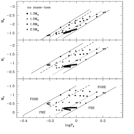
Figure 6: Selected Period-Magnitude diagrams of the predicted pulsators with $Z$=0.0001 and the labeled mass, in the absence of mass loss. The solid lines depict the blue (FOBE) and red (FRE) limits of the entire pulsator distribution, while the dashed and dotted lines are the blue edge for the fundamental (FBE) and the red edge for first overtone (FORE) pulsation, respectively. All the pulsators are plotted with their fundamental period, irrespective of the actual limits for the fundamental or first overtone pulsation mode (see text).

3 Pulsational relations

3.1 Period-Magnitude and Period-Color relations

In analogy with other radial pulsators such as RR Lyrae stars and Classical Cepheids, the pulsation period of ACs is uniquely defined by the intrinsic stellar parameters: mass, luminosity, and effective temperature. Based on the pulsation models presented by MFC and C04, for the fundamental (F) mode we adopt

$$\log P_{F}=10.88+0.82\log L-0.62\log M-3.31\log T_{e},$$

where the mass $M$ and the luminosity $L$ are in solar units. As for the first overtone (FO) period, from the MFC models we estimate that the average difference between the computed periods and the values obtained from equation (1) is log$P_{FO}$=log$P_{F}-$0.13, at constant mass, luminosity and effective temperature.

Table 4: Predicted boundaries in the Period-Magnitude diagram of the pulsator distribution with $Z$=0.0001 and $l/H_{p}$=1.5, in the absence of mass loss. The red (FRE) and blue (FBE) limits for fundamental pulsators are given as a function of the fundamental period $P_{F}$, while those (FORE and FOBE) for FO pulsators as a function of the first overtone period $P_{FO}$ (see text).

$M_{i}=a+b$log$P_{F}$
	FRE		FBE
$M_{i}$	$b$	$a$	$a$
$M_{V}$	$-$4.17	$-$0.20$\pm$0.08	$-$1.13$\pm$0.11
$M_{R}$	$-$4.27	$-$0.50$\pm$0.08	$-$1.35$\pm$0.11
$M_{I}$	$-$4.37	$-$0.85$\pm$0.07	$-$1.62$\pm$0.10
$M_{J}$	$-$4.50	$-$1.30$\pm$0.06	$-$1.93$\pm$0.08
$M_{K}$	$-$4.65	$-$1.65$\pm$0.05	$-$2.20$\pm$0.07
$M_{i}=a+b$log$P_{FO}$
	FORE		FOBE
$M_{i}$	$b$	$a$	$a$
$M_{V}$	$-$4.17	$-$1.05$\pm$ 0.13	$-$2.04$\pm$0.08
$M_{R}$	$-$4.27	$-$1.35$\pm$ 0.13	$-$2.26$\pm$0.08
$M_{I}$	$-$4.37	$-$1.69$\pm$ 0.11	$-$2.47$\pm$0.07
$M_{J}$	$-$4.50	$-$2.10$\pm$ 0.10	$-$2.69$\pm$0.06
$M_{K}$	$-$4.65	$-$2.47$\pm$ 0.08	$-$2.95$\pm$0.05

Adopting the fundamental period given by Eq. (1), we show in Fig. 6 selected Period-Magnitude ($PM$) diagrams for all the predicted pulsators in the absence of mass loss, as presented in Fig. 2. In this figure, the solid lines showing the limits of the pulsator distribution are the boundaries (FOBE and FRE) of the whole instability strip, adopting for all the pulsators the period corresponding to the fundamental mode. In reality, the MFC models show that within the instability strip there exist a blue edge for fundamental (FBE) and a red edge for first overtone pulsation (FORE), as given by log$T_{e}$(FBE)$-$log$T_{e}$(FRE)=0.055$\pm$0.005 and log$T_{e}$(FORE)$-$log$T_{e}$(FRE)=0.018$\pm$0.008, for fixed mass and luminosity. For effective temperatures between the FORE (FOBE) and the FRE (FBE) only the F (FO) mode is efficient, whereas between the FBE (dashed line in Fig. 6) and the FORE (dotted line in Fig. 6) both the pulsation modes are possible. However, if the first overtone period is adopted for FO pulsators, then both the FOBE and the FORE should be shifted by $\delta$log$P=-$0.13, with the result that the FORE and the FBE become almost coincident. This is shown in Table 4, where the limits for the fundamental pulsator distribution (FBE and FRE) are given as a function of $P_{F}$, while those for first overtone pulsators (FOBE and FORE) as a function of $P_{FO}$.

By inspection of Table 4 and Fig. 6, one has that the range in magnitudes, at a fixed period, expected for the predicted F or FO pulsators is quite large in the optical bands, decreasing when moving to longer wavelengths. Thus, synthetic $PM_{V}$ or $PM_{I}$ relations will significantly depend on the distribution of the pulsators within the pulsation region, at variance with the case of near-infrared magnitudes. In particular, the mean relations

$$M^{F}_{K}=-1.93(\pm 0.15)-4.65\log P_{F},$$

defined by all the F pulsators falling between the FBE and the FRE, and

$$M^{FO}_{K}=-2.71(\pm 0.18)-4.65\log P_{FO},$$

by all the FO pulsators between the FOBE and the FORE, can be used for distance determinations. Moreover, since in the $M_{K}$-log$P$ plane the dispersion at fixed periods depends almost entirely on the pulsator mass, we derive that the least-squares solution to all the $Z$=0.0001 pulsators, taken with their fundamental period, yields a quite tight mass-dependent $PM_{K}$ relation, as given by

$$M_{K}=-1.40(\pm 0.04)-2.44\log P_{F}-2.57\log M,$$

Figure 7: Selected Period-Color diagrams of the pulsators with $Z$=0.0001 and the labeled mass, in the absence of mass loss. The solid lines depict the limits (FOBE and FRE) of the entire instability strip, while the dashed and the dotted lines are the blue edge for fundamental (FBE) and the red edge for first overtone (FORE) pulsation, respectively. Note that all the pulsators and the pulsation edges are plotted with the fundamental period.

Table 5: As in Table 4, but for the Period-Color diagrams.

$[CI]=a+b$log$P_{F}$
	FRE		FBE
$[CI]$	$b$	$a$	$a$
$M_{B}-M_{V}$	0.17	0.45$\pm$0.03	0.29$\pm$0.04
$M_{V}-M_{R}$	0.10	0.32$\pm$0.03	0.21$\pm$0.04
$M_{V}-M_{I}$	0.20	0.67$\pm$0.04	0.46$\pm$0.06
$M_{V}-M_{J}$	0.35	1.09$\pm$0.05	0.76$\pm$0.07
$M_{V}-M_{K}$	0.50	1.48$\pm$0.06	1.02$\pm$0.08
$[CI]=a+b$log$P_{FO}$
	FORE		FOBE
$[CI]$	$b$	$a$	$a$
$M_{B}-M_{V}$	0.17	0.42$\pm$0.05	0.25$\pm$0.03
$M_{V}-M_{R}$	0.10	0.29$\pm$0.05	0.18$\pm$0.03
$M_{V}-M_{I}$	0.20	0.64$\pm$0.06	0.41$\pm$0.04
$M_{V}-M_{J}$	0.35	1.04$\pm$0.08	0.70$\pm$0.05
$M_{V}-M_{K}$	0.50	1.42$\pm$0.10	0.94$\pm$0.06

For the Period-Color ($PC$) diagram, Fig. 7 shows that the dispersion of the pulsator distribution, at fixed period, increases moving from $B-V$ to $V-K$ colors. As a consequence we find that only the mean optical relations derived from all the predicted F pulsators

$$[M_{B}-M_{V}]^{F}=0.37(\pm 0.05)+0.17\log P_{F}$$

$$[M_{V}-M_{I}]^{F}=0.57(\pm 0.07)+0.20\log P_{F}$$

and the ones derived for FO pulsators

$$[M_{B}-M_{V}]^{FO}=0.34(\pm 0.07)+0.17\log P_{FO}$$

$$[M_{V}-M_{I}]^{FO}=0.52(\pm 0.09)+0.20\log P_{FO}$$

appear useful for reddening determinations. We notice that in this case, as reported in Table 5, the adoption of the first overtone period for FO pulsators will leave a FORE significantly redder than the blue edge of F pulsators, taken with their fundamental period.

3.2 Period-Magnitude-Color relations

The application of Eq. (1) in the observational plane is a mass-dependent Period-Magnitude-Color relation (hereafter, named $PMC$) in which the pulsator absolute magnitude is strictly correlated with period and color, for any given mass. A linear regression through the magnitudes and the fundamental periods of all the predicted pulsators generated in the absence of mass loss yields the mass-dependent $PMC$ relations listed in Table 6.

Table 6: Mass-dependent $PMC$ relations. In the last column, we give the total intrinsic dispersion $\pm\sigma_{V}$.

$M_{V}=a+b$log$P_{F}+c[CI]+d$log$M$
$[CI]$	$a$	$b$	$c$	$d$	$\sigma_{V}$
$M_{B}-M_{V}$	$-$1.75	$-$2.86	3.99	$-$2.02	0.03
$M_{V}-M_{R}$	$-$1.86	$-$2.99	5.92	$-$1.88	0.03
$M_{V}-M_{I}$	$-$1.99	$-$3.02	2.96	$-$1.85	0.03
$M_{V}-M_{J}$	$-$2.01	$-$3.03	1.93	$-$1.88	0.03
$M_{V}-M_{K}$	$-$1.93	$-$3.02	1.29	$-$1.90	0.03

Figure 8: Left panels - Behavior of $Z$=0.0001 pulsators with $M$=1.5$M_{\odot}\,$as generated in the absence of mass loss (solid line) or by a progenitor with 2.0$M_{\odot}\,$(dashed line). In the lower two panels, we plot the luminosity versus the effective temperature and the visual magnitude versus the fundamental period, while the upper panel deals with the $PMC$ relation given in Table 6. Right panels - As in the left panels, but with 2.0$M_{\odot}\,$pulsators with $Z$=0.0001 (solid line) and $Z$=0.0004 (dashed line), in the absence of mass loss.

The mass-dependent relations hold for all the combinations of mass and luminosity, thus they are not influenced by the occurrence of mass loss before or during the He-burning phase. As an example, the left panels in Fig. 8 show the comparison between the 1.5$M_{\odot}\,$model without mass loss ($M_{He}$=0.463$M_{\odot}\,$, solid line) and the 1.5$M_{\odot}\,$structure generated by a 2.0$M_{\odot}\,$progenitor ($M_{He}$=0.416$M_{\odot}\,$, dashed line) which lost 0.5$M_{\odot}\,$. According to the different He-core masses, the two models evolve at different bolometric luminosities and they follow distinct behaviors in the $M_{V}$-log$P_{F}$ plane (lower two panels), with an average visual magnitude $M_{V}\sim-$0.41 mag and $\sim-$0.28 mag without and with mass loss, respectively. However, the effects of such a luminosity variation on the $PMC$ relation (upper panel) are zero. Similar results are derived when the variation in luminosity is due to a different metal content, at least in the range $Z$=0.0001-0.0004. This is shown in the right panels in Fig. 8, where the comparison between 2.0$M_{\odot}\,$models with $Z$=0.0001 (solid line) and $Z$=0.0004 (dashed line) is presented. Later, we will give a full discussion of the metallicity effects on the various pulsational relations.

The constraints provided by the evolution theory, and in particular the occurrence of a $ML$ relation that binds the permitted values of mass and luminosity of the predicted pulsators, allow us to derive “evolutionary” $PMC$ relations (hereafter $PMC_{e}$) where the mass-term is removed. Obviously these relations are expected to depend on the assumption on the amount of mass loss.

Table 7: Evolutionary $PMC_{e}$ relations for $Z$=0.0001 pulsators in the mass range 1.3-2.0$M_{\odot}\,$, in the absence of mass loss.

$M_{V}=\alpha_{0}+\beta_{0}$log$P_{F}+\gamma_{0}[CI]$
[CI]	$\alpha_{0}$	$\beta_{0}$	$\gamma_{0}$
$M_{B}-M_{V}$	$-$2.54$\pm$0.08	$-$4.05$\pm$0.06	4.91$\pm$0.10
$M_{V}-M_{R}$	$-$2.71$\pm$0.08	$-$4.18$\pm$0.06	7.58$\pm$0.16
$M_{V}-M_{I}$	$-$2.89$\pm$0.08	$-$4.21$\pm$0.06	3.82$\pm$0.08
$M_{V}-M_{J}$	$-$3.02$\pm$0.08	$-$4.30$\pm$0.06	2.48$\pm$0.05
$M_{V}-M_{K}$	$-$3.00$\pm$0.08	$-$4.37$\pm$0.06	1.82$\pm$0.03

For the sample of $Z$=0.0001 pulsators with mass 1.3, 1.5, 1.8 and 2.0$M_{\odot}\,$in the absence of mass loss, i.e., in the case of a mass variation due to different evolutionary ages (see $t$ values in Table 1), a linear regression through all the predicted pulsators, taken with their fundamental period, yields the $PMC_{e}$ relations given in Table 7. These relations can be used to determine the distance to individual Cepheids with a formal accuracy of $\sim$ 0.1 mag, provided that the intrinsic colors are known with the adequate accuracy.

Figure 9: As in Fig. 6, but for the predicted pulsators with a mean mass $\langle M\rangle$=1.3$M_{\odot}\,$, as generated by a 2.0$M_{\odot}\,$progenitor star. The solid lines depict the limits (FOBE and FRE) of the whole instability strip in absence of mass loss.

Figure 10: As in Fig. 7, but for the predicted pulsators with a mean mass $\langle M\rangle$=1.3$M_{\odot}\,$, as generated by a 2.0$M_{\odot}\,$progenitor star. The solid lines show the limits (FOBE and FRE) of the IS in the absence of mass loss.

For coeval pulsators whose mass variation is due to different amounts of mass loss suffered by the same progenitor star, we show in Fig. 9 and Fig. 10 the $PM$ and $PC$ distributions of the synthetic pulsators with a mean mass $\langle M\rangle$=1.3$M_{\odot}\,$, as generated by a mass loss of $\sim$ 0.7$M_{\odot}\,$in a 2.0$M_{\odot}\,$progenitor star. For a given mass, these pulsators are fainter than those originating in the absence of mass loss and that following such a luminosity decrease the pulsation edges move towards larger effective temperatures, i.e., shorter periods. Eventually, these two effects yield that the whole $PM$ distribution is on average brighter by about 0.1 mag than that in absence of mass loss (solid lines), for a fixed metal content. Concerning the $PC$ distribution, the concomitant variation of color and period causes the limits of the instability strip to be not significantly different from those in the absence of mass loss (solid lines).

Table 8: Evolutionary $PMC_{e}$ relations for $Z$=0.0001 pulsators generated by mass loss in a 2.0$M_{\odot}\,$progenitor star.

$M_{V}=\alpha+\beta$log$P+\gamma[CI]$
[CI]	$\alpha$	$\beta$	$\gamma$
$M_{B}-M_{V}$	$-$2.36$\pm$0.06	$-$3.15$\pm$0.06	4.61$\pm$0.04
$M_{V}-M_{R}$	$-$2.55$\pm$0.06	$-$3.45$\pm$0.06	7.12$\pm$0.06
$M_{V}-M_{I}$	$-$2.71$\pm$0.06	$-$3.52$\pm$0.06	3.58$\pm$0.03
$M_{V}-M_{J}$	$-$2.87$\pm$0.06	$-$3.68$\pm$0.06	2.34$\pm$0.02
$M_{V}-M_{K}$	$-$2.86$\pm$0.06	$-$3.79$\pm$0.06	1.72$\pm$0.01

For the $PMC_{e}$ relations in the presence of mass loss, the linear regression through the various synthetic populations presented in Fig. 4 shows that the coefficients are slightly dependent on the mass of the progenitor star. Using all the predicted pulsators generated by a 2.0$M_{\odot}\,$progenitor, we find the coefficients listed in Table 8. Moreover, we find that these relations hold also with $M_{pr}$=1.5$M_{\odot}\,$and 1.8$M_{\odot}\,$, with only the constant term depending on the mass, or age, of the progenitor star as $\delta\alpha$=$-$0.16($M_{pr}-$2.0).

Figure 11: As in Fig. 1, but for 2.0$M_{\odot}\,$evolutionary tracks with the labeled metal content, in absence of mass loss.

Figure 12: (upper panel) - Minimum mass for the occurrence of massive central He-burning pulsators as a function of the metal content. (lower panel) - Predicted faintest magnitude ($M_{V,LE}$) of the massive pulsators as a function of metal content.

3.3 Metallicity effects and mean magnitudes

In order to discuss the effects of the metal content on the various pulsational relations, we first present some basic evolutionary constraints. This issue has been discussed in previous papers (see C04 and references therein); in Fig. 11 the behavior of selected evolutionary tracks (Cariulo, Degl’Innocenti & Castellani 2004) with $M$=2.0$M_{\odot}\,$and metal content varying from $Z$=0.0002 to $Z$=0.001, are shown to highlight that the blueward extension of the central He-burning path becomes fainter and redder with increasing the metal content, at a given mass. As a consequence, the minimum mass evolving from the ZAHB turnover into the IS, namely the minimum mass for the occurrence of massive central He-burning pulsators, increases with increasing $Z$, passing from $\sim$ 1.2$M_{\odot}\,$at $Z$=0.0001 to $\sim$ 1.7$M_{\odot}\,$with $Z$=0.0004 and to $\sim$ 2.2$M_{\odot}\,$with $Z$=0.001 (see upper panel in Fig. 12). Correspondingly, the lower luminosity level ($M_{V,LE}$) of the massive pulsators increases from $\sim-$0.1 mag ($Z$=0.0001) to $\sim-$0.5 mag at $Z$=0.0004 and $\sim-$0.8 mag at $Z$=0.001 (see lower panel in Fig. 12 as well as Fig. 7 in C04). Thus, the intrinsically faint ACs observed around $\sim$ 0 mag (see following Section 4) imply that the metal content cannot be larger than $Z\sim$ 0.0004.

An increase of the metal content from $Z$=0.0001 to $Z$=0.0004 reveals that the average luminosity of the predicted AC pulsators with a given mass decreases as $\Delta$log$L\sim-$0.1. The effects of such a luminosity variation on the boundaries of the IS are similar to those discussed in the case of mass loss: the $PM$ distribution, and the limits given in Table 4, become brighter by about 0.1 mag, while the effects on the $PC$ distribution are negligible. Concerning the evolutionary $PMC_{e}$ relations, we derive that the correction to the $Z$=0.0001 zero-points ($\alpha_{0}$ in Table 7 and $\alpha$ in Table 8) are $\sim-$0.10 mag.

The magnitudes computed so far are the static values the stars would have if they were not pulsating, whereas the measurements deal with time-averaged quantities over a pulsation period. The mean values may be significantly different from the static ones (see , e.g., MFC; Marconi et al. 2003; Di Criscienzo, Marconi & Caputo 2004) and thus the coefficients of the mass-dependent $PMC$ relations we give in Table 6 are slightly different from those derived by MFC on the basis of intensity-averaged magnitudes of the pulsation models (see their Table 3). The mass-dependent $PMC$ relations provided by MFC, as based on intensity-weighted magnitudes, should be preferred to estimate the mass of individual variables with well-measured absolute magnitudes and intrinsic colors; alternatively, if the intrinsic color and the mass are known, they give accurate individual distances.

For near-infrared bands the discrepancy between static and mean values is always insignificant. In summary, the boundaries given in Table 5 and Table 6 and the mean relations derived in Section 3.1 can be safely compared with measured intensity-weighted magnitudes, whereas the effects on the $PMC_{e}$ relations dealing with optical colors may reach significant values. As an example, the quantity $\langle V\rangle-\gamma_{0}[\langle B\rangle-\langle V\rangle$] may be up to $\sim$ 0.14 mag fainter than the corresponding static value.

Figure 13: Color-Magnitude diagram of observed ACs (filled circles) compared to the predicted boundaries given in Table 2 (solid lines).

Figure 14: Color-Magnitude diagram of observed ACs (filled circles) compared to the predicted boundaries given in Table 2. We plot also short-period Classical Cepheids (spCC: open squares) and Population II Cepheids (P2C: open triangles).

4 Comparison with observations

For the dwarf galaxies listed in Table 9, Figs. 13 and 14 show the intensity-weighted absolute magnitude of the observed ACs (filled circles) versus the intrinsic color together with the predicted limits of the instability strip (solid lines), as given in Table 2. Although these limits hold with $Z$=0.0001 in the absence of mass loss, we have already shown that even with a mass loss of $\sim$ 0.7$M_{\odot}\,$the color shift is only $\sim-$0.03 mag (see Fig. 5) and that the metallicity effect is negligible. The errorbars are drawn adopting a photometric error of $\pm$0.05 mag on each mean magnitude and an uncertainty of 0.15 mag on the intrinsic distance modulus. This yields $\epsilon(M_{V})=\pm$0.16 mag and $\epsilon(CI)=\pm$0.07 mag.

Table 9: Dwarf galaxies with observed Anomalous Cepheids listed with their intrinsic distance modulus $\mu_{0}$, $E(B-V)$ reddening, and metal abundance [Fe/H].

galaxy	$\mu_{0}$	$E{B-V}$	[Fe/H]	Ref.	Notes
	(mag)	(mag)
AndI	24.5	0.05	$-$1.5	1	a
AndII	24.1	0.06	$-$1.5	2	a
AndIII	24.3	0.06	$-$1.9	1	a
AndVI	24.5	0.06	$-$1.6	3	a
Carina	20.1	0.04	$-$1.6	4	a
Draco	19.5	0.03	$-$2.1	3	a
Fornax	20.7	0.03	$-$1.6	5	b,e
LeoII	21.6	0.02	$-$1.9	3,6	c
LMC	18.5	0.10	$-$1.7	7	a,f
Phoenix	23.1	0.02	$-$1.4	8	d,f
Sculptor	19.6	0.02	$-$1.8	9,10	c
Sextans	19.7	0.04	$-$1.6	11	a

References - (1): Pritzl et al. 2005; (2): Pritzl et al. 2004; (3): Pritzl et al. 2002; (4): Dall’Ora et al. 2003; (5): Bersier & Wood 2002; (6): Siegel & Majewski 2000; (7): Di Fabrizio et al. 2005; (8): Gallart et al. 2004; (9): Kaluzny et al. 1995; (10): Clementini et al. 2005; (11): Mateo, Fischer & Krzeminski 1995. Notes - (a): $B,V$ data; (b): $V,I$ data; (c): $V$ data; (d): $B,V,I$ data; (e) Population II Cepheids also observed; (f): Short-period Classical Cepheids also observed.

In Fig. 13, we find an agreement between the observed $CM$ distribution and the predicted limits (FOBE and FRE) of the instability strip, with the only exception of v1 in AndIII whose color is significantly bluer than the predicted FOBE. As for the galaxies in Fig. 14, the agreement is less because of the several ACs (filled circles) located out of the predicted IS (see column (2) in Table 10). However, in this diagram the observed Population II Cepheids (P2C: open triangles) are not clearly separated from ACs, while the short-period Classical Cepheids (spCC: open squares) agree with the AC boundaries extended to brighter magnitudes.

Figure 15: Period-Color diagram of observed ACs (filled circles) compared to the predicted boundaries for F and FO pulsators, as given in Table 5.

Figure 16: Period-Color diagram of observed ACs (filled circles) compared to the predicted boundaries for F and FO pulsators, as given in Table 5. We plot also short-period Classical Cepheids (spCC: open squares) and Population II Cepheids (P2C: open triangles).

For the $PC$ diagrams, Figs. 15 and 16 show the intrinsic colors versus the observed periods in compared to the predicted limits.

For the galaxies plotted in Fig. 15, we find an agreement between the observed distribution and the predicted FOBE and FRE, with the exception of variable v1 in AndIII, which is bluer than the FOBE, and v19 and v34 in Sextans, which appear somehow redder than the FRE. Concerning the galaxies in Fig. 16, we have again a significant number of variables lying out of the predicted IS, as listed in column (3) of Table 10.

Figure 17: Period-Magnitude diagram of observed ACs (filled circles) in comparison with the predicted boundaries for F and FO pulsators, as given in Table 4, corrected for metallicity.

Figure 18: Period-Magnitude diagram of observed ACs (filled circles) in comparison with the predicted boundaries for F and FO pulsators, as given in Table 4, corrected for metallicity. We plot also short-period Classical Cepheids (spCC: open squares) and Population II Cepheids (P2C: open triangles). The solid lines are the predicted boundaries given in Table 4 corrected for metallicity.

Figs. 17 and 18 show the absolute magnitudes versus the observed period. In this case, since the zero-points listed in Table 4 hold in the absence of mass loss and with $Z$=0.0001, i.e., at [Fe/H]=$-$2.1 referenced to $Z_{\odot}$=0.012 (Asplund et al. 2005), they are corrected for the metal content of the variables adopting $\delta a=-$0.17([Fe/H]+2.1). As for the effects of mass loss, we recall that the predicted limits become brighter by $\sim$ 0.1 mag with a mass loss of $\sim$ 0.7$M_{\odot}\,$.

For all the galaxies, we now find an excellent agreement with the predicted FOBE and FRE, with very few exceptions: the variables v1 in AndI, v8 in AndIII and (by a minor extent) J023952.5 in Fornax, which are fainter than the FRE, and the variables v193 in Carina and v10320 in LMC, wich are slightly brighter than the FOBE. As already shown in Table 4, in this plane the predicted blue edge for fundamental pulsators (FBE, dashed line) is almost coincident with the red edge for first overtone pulsators (FORE, dotted line). Taking into account the uncertainty of the predicted edges ($\sim$ 0.12 mag) and of the measured magnitudes ($\sim$ 0.16 mag), we preliminarily assign the fundamental mode (F) to the variables $\geq$ 0.2 mag fainter than FORE and the first overtone mode (FO) to those $\geq$ 0.2 mag brighter than the FBE, leaving the few remaining variables with an uncertain (FFO) classification. ACs (filled circles) and spCCs (open squares) in LMC and Phoenix populate a rather common instability strip, with the latter variables located at brighter magnitudes and longer periods. Conversely, the P2Cs observed in Fornax have a distinct behavior, being significantly fainter than the AC fundamental red edge. Such evidence leads us to suppose that v1 in AndI and v8 in AndIII might be Population II Cepheids, as already suggested by Pritzl et al. (2005).

Table 10: Anomalous Cepheids not fulfilling the predicted edges of the instability strip into the Color-Magnitude ($CM$), Period-Color ($PC$) or Period-Magnitude ($PM_{V}$) diagram. The label “yes” means that the variable agree with the predicted edges in a given diagram, otherwise we give the reason for the disagreement.

gal/var	$CM$	$PC$	$PM_{V}$
AndI
1	$B-V<$FOBE	yes	$M_{V}>$FRE
AndIII
1	yes	$B-V<$FOBE	yes
8	yes	yes	$M_{V}>$FRE
Carina
193	yes	yes	$M_{V}<$FOBE
Fornax
J0+
24050.2	$V-I>$FRE	$V-I>$FRE	yes
23907.1	$V-I>$FRE	$V-I>$FRE	yes
24002.7	$V-I>$FRE	$V-I>$FRE	yes
23937.7	$V-I>$FRE	$V-I>$FRE	yes
23946.2	$V-I>$FRE	$V-I>$FRE	yes
23952.5	$V-I>$FRE	$V-I>$FRE	$M_{V}>$FRE
LMC
10320	yes	$B-V>$FRE	$M_{V}<$FOBE
9578	$B-V>$FRE	$B-V>$FRE	yes
5952	$B-V>$FRE	$B-V>$FRE	yes
Phoenix
103951	$B-V<$FOBE	$B-V<$FOBE	yes
6793	$V-I>$FRE	$V-I>$FRE	yes
11219	$B-V<$FOBE	$B-V<$FOBE	yes
10800			yes
Sextans
34	yes	$B-V>$FRE?	yes
19	yes	$B-V>$FRE?	yes

Figure 19: Period-Magnitude-Color distribution of observed ACs compared to the predicted relation for F and FO pulsators, in the absence of mass loss. Filled and open circles are F and FO pulsators, respectively, while the circled dots refer to FFO variables. The open triangles show the suspected P2Cs.

Figure 20: As in Fig. 23, but for the variables in LMC. The asterisks refer to the AC candidates not fullfilling the predicted instability strip requirements (see Table 10). The open squares show spCCs.

Figure 21: As in Fig. 23, but for the observed ACs in Phoenix and Fornax. We plot also spCCS (open squares) and P2Cs (open triangles).

The results of the comparison between the observed $CM$, $PC$ and $PM$ distributions and the predicted edges of the whole instability strip, as summarized in Table 10, show that each of these bi-dimensional diagrams can yield discordant results. This is not a surprise since the properties of individual variables are fully described by a four-dimensional formulation as given by Eq. (1) or, in the case of variables following the same $ML$ relation, by the three-dimensional one provided by the $PMC_{e}$ relation.

Using only the variables filling the predicted instability strip, i.e., excluding those listed in Table 10, and adopting the coefficients given in Table 7 to correct the absolute magnitude for the color, we show in Figs. 19-21 the comparison with the predicted $PMC_{e}$ relations in absence of mass loss. In these figures, the F and FO pulsators identified in the $PM_{V}$ diagram are plotted with filled and open circles, respectively, while the circled dots refer to FFO pulsators. Moreover, the predicted $PMC_{e}$ relations, which are given at $Z$=0.0001 as a function of $P_{F}$, are corrected for the metal content adopting $\delta\alpha_{0}=-$0.17([Fe/H]+2.1) and are also plotted shifted by $\delta$log$P=-$0.13 to account for FO pulsators. The errorbars are drawn to account for the photometric errors [$\epsilon(M_{V})=\pm$0.16 mag and $\epsilon(B-V)=\epsilon(V-I)\pm$0.07 mag] and the intrinsic uncertainty ($\pm$ 0.08 mag) of the predicted $PMC_{e}$ relations.

Inspection of the figures yields the following results:

• AndI: We can definitely conclude that v1 is a P2C

• AndII: We confirm that v14 is a FO pulsator;

• AndIII: The variable v8 is a P2C. The two FO candidates v6 and v7 are located above the predicted $PMC_{e}$ relation, suggesting that the measured $B-V$ color is too red or the adopted distance modulus too long. In the latter case, a difference $\delta\mu_{0}\sim-$ 0.3 mag would yield a statistical agreement, as well as the assignment of the fundamental mode to the variable v9. Otherwise, if the measured colors and the adopted distance modulus are correct, v6 and v7 are not ACs and no safe pulsation mode can be assigned to v9;

• AndVI: All the observed ACs agree with the predicted relations, but no clear pulsation mode can be assigned to the FFO variable v93 (classified as F by MFC);

• Sextans: There is a statistical agreement with the predicted relations;

• Carina: All the F and FO candidates agree quite well with the predicted relations. The FFO variable v33 is a FO pulsator, in agreement with MFC;

• Draco: All the F and FO candidates agree with the predicted relations. The FFO variable v157 is a FO pulsator, as suggested by MFC;

• LMC: The three AC candidates not fitting in the predicted edges of the IS (asterisks) are clearly at odds with the predicted $PMC_{e}$ relations, while a marginal agreement is found for the remaining fundamental candidate v9604. The observed spCCs (open squares) are fitted once the typical metal content of the Classical Cepheids in LMC ([Fe/H]=$-$0.4, i.e., $Z$=0.005) is taken into consideration;

• Phoenix: Adopting $V-I$ colors, which give less noisy results than $B-V$ ones, we derive that all the ACs, except v3441, would agree with the predicted $PMC_{e}$ relations if a slightly larger distance modulus ($\delta\mu_{0}\sim$ 0.2 mag) were adopted. This is also supported by the observed spCCs (open squares). In such a case, v12003 is a FO pulsator, whereas the peculiar location of v3441 above the FO predicted relation would suggest that the measured color is too red;

• Fornax: All the ACs are in reasonable agreement with the predicted relations, and we can assign the first overtone mode to J023926.8 and J024058.3, while J023941.5 and J024016.9 are pulsating in the fundamental mode. The P2Cs (open triangles) are located at significantly longer periods than the fundamental $PMC_{e}$ relation, except J023811.9 whose color [$(V-I)_{0}$=1.06 mag) is more than 0.4 mag redder than the other P2Cs.

Figure 22: Safe AC candidates in the Period-Magnitude diagram, with the visual magnitude corrected for the metal content. The solid lines are the best fit to the data.

Similar results are obtained in the case of mass loss, i.e., by using the predicted $PMC_{e}$ relations given in Table 8. The AC candidates which satisfy the predicted edges of the IS in the $CM$, $PC$ and $PM_{V}$ diagram can be used to obtain empirical $PM_{V}$ relations. This is shown in Fig.22, where $\langle M_{V}\rangle_{Z}$=$\langle M_{V}\rangle$+0.17([Fe/H]+2.1) and the solid lines are the linear regression through the points

$$M_{V,Z}^{F}=-0.58-2.74\log P_{F}$$

$$M_{V,Z}^{FO}=-1.31-3.13\log P_{FO}$$

as derived giving to the FFO pulsators a half weight with respect to safe F and FO variables. These relations are in good agreement with the ones presented in MFC for a smaller sample of pulsators and neglecting the metallicity effect.

5 Conclusions

We have presented an homogeneous and updated theoretical scenario for the study of AC properties based on a new set of evolutionary tracks with $Z$=0.0001, progenitor mass in the range 1.3-2 $M_{\odot}\,$and several assumptions on the efficiency of mass loss. This evolutionary framework is related to the pulsation model predictions by MFC. We find that predicted pulsators with mass 1.3-2.0 $M_{\odot}$ follow a ML relation as given by $\langle$log$L\rangle\sim$ 1.77($\pm$0.05)+2.07log$M$, in absence of mass loss. Moreover, the evolutionary and pulsational models have been used to build synthetic populations of AC pulsators, each characterized by a progenitor mass, a mean mass and a percentage of central He-burning stars populating the IS. We find that pulsators with a given mass originating in the presence of mass loss are systematically fainter than the ones in the absence of mass loss, with the decrease in luminosity following the variation in the He-core mass. We have also investigated the effect of mass loss on the predicted IS boundaries in the $CM$, $PC$ and $PM$ planes and we find that the only significant dependence occurs in the $PM$ plane where the synthetic distribution in the presence of mass loss is, on average, brighter by about 0.1 mag than the one in the absence of mass loss.

Concerning the existence of a $PM$ relation for these stars, we confirm that in the case of optical magnitudes it depends on the pulsator distribution within the IS, whereas tight near-infrared $PM_{K}$ relations can be derived for both fundamental and first overtone pulsators, providing a reliable tool for distance evaluations with an intrinsic uncertainty of about 0.15 mag. If the mass term is taken into account a tighter (mass-dependent) PM_K relation (r.m.s=0.04 mag.) is obtained. Conversely, the predicted $PC$ relations dealing with $B-V$ and $V-I$ colors appear useful for reddening determinations with an intrinsic uncertainty of less than 0.1 mag. Mass-dependent $PMC$ relations have been derived by using all the models, as well as evolutionary $PMC_{e}$ relations where the mass-term is removed. The latter relations allow distance determinations with a formal uncertainty of the order of 0.1 mag, provided that the intrinsic colors are well known.

To take into account the metallicity effect, we have used other evolutionary tracks from the literature with $Z$ in the range 0.0001-0.001. In particular, we find that an increase of the metal content from 0.0001 to 0.0004 yields that, at fixed mass, the average luminosity of predicted AC pulsators decreases by $\sim$ 0.1 dex, producing an effect on the IS boundaries similar to the one due to mass loss, whereas the zero-points of the predicted $PMC_{e}$ relations becomes brighter by $\sim$ 0.1 mag.

By comparing the predicted edges of the IS with observed pulsators in the $CM$, $PC$ and $PM$ planes, we find discordant results in the properties of individual stars, thus confirming that a sure identification of actual ACs requires simultaneous information on period, magnitude and color through the application of the predicted $PMC_{e}$ relations. In this case, we are also able to provide constraints on the pulsation mode. We show that AC candidates that satisfy the predicted edges of the IS in the $CM$, $PC$ and $PM_{V}$ diagrams can be used to obtain empirical $PM_{V}$ relations for F and FO pulsators.

- (1) Asplund, M., Grevesse, N., Sauval, A.J., Allende Prieto, C., & Kiselman, D., 2004, A&A, 417, 751A
- (2) Bersier, D. & Wood, P.R., 2002, AJ, 123, 840B
- (3) Bessell, M.S. & Brett, J.M., 1988, PASP, 100, 1134B
- (4) Bono, G., 2003, in Stellar Clandles for the Extragalactic Distance Scale, ed. D. Alloin and W. Gieren (Berlin: Springer Verlag), 85
- (5) Bono, G., Caputo F., Castellani V., Marconi M., Storm J., 2001, MNRAS, 326, 1183-1190
- (6) Bono, G., Caputo, F., Santolamazza, P., Cassisi, S., Piersimoni, A., 1997, AJ, 113, 1109B
- (7) Bono, G. & Stellingwerf, R.F., 1994, ApJS, 93, 233B
- (8) Caputo, F., 1998, A&ARv, 9, 33C
- (9) Caputo F., Castellani V., Degl’Innocenti S., Fiorentino G., Marconi M., 2004, A&A, 424, 927C
- (10) Cardelli, J.A., Clayton, G.C., & Mathis, J.S., 1989, ApJ, 345, 245C
- (11) Cariulo, P., Degl’Innocenti, S., & Castellani, V., 2004, A&A, 421, 1121C
- (12) Castellani, V., & Degl’Innocenti, S. 1995, A&A, 298, 832
- (13) Castelli, F., Gratton, R. G., & Kurucz, R. L. 1997a, A&A, 318, 841
- (14) Castelli, F., Gratton, R. G., & Kurucz, R. L. 1997a, A&A, 318, 841
- (15) Clementini, G., Held, E.V., Baldacci, L. & Rizzi, L., 2003, ApJ, 588L, s85C
- (16) Clementini, G., Ripepi, V., Bragaglia, A., Fiorenzano, A.F.M., Held, E.V. & Gratton, R.G., 2005, MNRAS, 363, 734C
- (17) Cordier, D., Goupil, M.J. & Lebreton, Y., 2003, A&A, 409, 491C
- (18) Cousins, A.W.J., 1980, SAAOC, 1, 234C
- (19) Dall’Ora, M., Ripepi, V., Caputo, F., Castellani, V., Bono, G., Smith, H.A., Brocato, E., Buonanno, R., Castellani, M., Corsi, C.E., Marconi, M., Monelli, M., Nonino, M., Pulone, L. & Walker, A.R., 2003, AJ, 126, 197D
- (20) Di Criscienzo, M., Marconi, M. & Caputo, F., 2004, ApJ, 612, 1092D
- (21) Di Fabrizio, L., Clementini, G., Maio, M., Bragaglia, A., Carretta, E., Gratton, R., Montegriffo, P. & Zoccali, M., 2005, A&A, 430, 603D
- (22) Dolphin, A.E. Saha, A. Claver, J., Skillman, E.D., Cole, A.A., Gallagher, J.S., Tolstoy, E., Dohm-Palmer, R.C., & Mateo, M., 2002, AJ, 123, 3154D
- (23) Dolphin, A.E., Saha, A., Skillman, E.D., Dohm-Palmer, R.C., Tolstoy, E., Cole, A.A., Gallagher, J.S., Hoessel, J.G. & Mateo, M., 2003, AJ, 125, 1261D
- (24) Gallart, C., Aparicio, A., Freedman, W.L., Madore, B.F., Martínez-Delgado, D. & Stetson, P.B., 2004, AJ, 127, 1486G
- (25) Kaluzny, J., Kubiak, M., Szymanski, M., Udalski, A., Krzeminski, W. & Mateo, M., 1995A&AS, 112, 407K
- (26) Limongi, M., & Chieffi, A. 2003, ApJ, 592, 404
- (27) Marconi, M., Caputo, F., Di Criscienzo, M., & Castellani, M., 2003, ApJ, 596, 299M
- (28) Marconi, M., Fiorentino, G., & Caputo, F. 2004, A&A, 417, 1101
- (29) Mateo, M., Fischer, P., & Krzeminski, W., 1995, AJ, 110, 2166M
- (30) Norris, J., & Zinn, R., 1975, ApJ, 202, 335N
- (31) Nemec, J.M., Nemec, A.F.L. & Lutz, T.E., 1994, AJ, 108, 22ss2N
- (32) Pritzl, B.J., Armandroff, T.E., Jacoby, G.H., & Da Costa, G.S., 2002, AJ, 124, 1464P
- (33) Pritzl, B.J., Armandroff, T.E., Jacoby, G.H., & Da Costa, G.S., 2004, AJ, 127, 318P
- (34) Pritzl, B.J., Armandroff, T.E., Jacoby, G.H. & Da Costa, G.S., 2005, AJ, 129, 2232P
- (35) Pietrinferni, A, Cassisi, S., Salaris, M., & Castelli, F., ApJ, 612, 168
- (36) Siegel, M.H. & Majewski, S.R., 2000, AJ, 120284S
- (37) Smith, H. A. & Stryker, L.L., 1986, AJ, 92, 328S
- (38) Stellingwerf, R.F., 1982, ApJ, 262, 330S
- (39) Zinn, R. & Searle, L.1976, ApJ, 209, 734Z