The Mid-IR Properties of Starburst Galaxies from Spitzer-IRS Spectroscopy

Abstract

We present $5-38\mu$m mid-infrared spectra at a spectral resolution of $R\approx 65-130$ of a large sample of 22 starburst nuclei taken with the Infrared Spectrograph IRS on board the Spitzer Space Telescope. The spectra show a vast range in starburst SEDs. The silicate absorption ranges from essentially no absorption to heavily obscured systems with an optical depth of $\tau_{9.8\mu m}\sim 5$. The spectral slopes can be used to discriminate between starburst and AGN powered sources. The monochromatic continuum fluxes at $15\mu$m and $30\mu$m enable a remarkably accurate estimate of the total infrared luminosity of the starburst. We find that the PAH equivalent width is independent of the total starburst luminosity $L_{IR}$ as both continuum and PAH feature scale proportionally. However, the luminosity of the $6.2\mu$m feature scales with $L_{IR}$ and can be used to approximate the total infrared luminosity of the starburst. Although our starburst sample covers about a factor of ten difference in the [Ne III] / [Ne II] ratio, we found no systematic correlation between the radiation field hardness and the PAH equivalent width or the $7.7\mu$m / $11.3\mu$m PAH ratio. These results are based on spatially integrated diagnostics over an entire starburst region, and local variations may be “averaged out”. It is presumably due to this effect that unresolved starburst nuclei with significantly different global properties appear spectrally as rather similar members of one class of objects.

1. Introduction

Many nearby galaxies show dramatically increased rates of star formation compared with the Milky Way. In such ”Starburst” galaxies (e.g., Weedman et al. (1981)), the primary energy source is driven by high nuclear star formation rates, rapid nuclear gas depletion time-scales and high supernovae rates. Such starburst systems often, though not exclusively, occur in interacting and colliding systems. Since collisions and interactions are believed to be a fundamental part of the evolution of galaxies by hierarchical growth, the full characterization of starburst galaxies is of the great importance in measuring and quantifying the global history of star formation over cosmic time. Determining the average mid-infrared (mid-IR) spectral properties, and the range of observed behavior within the starburst class at low redshift is vital for interpreting spectra of higher redshift IR sources, providing complementary spectral templates to those parallel Spitzer studies of the more extreme ULIRG systems (e.g., Armus et al. (2006b)) and AGN (e.g., Weedman et al. (2005)).

The term “starburst galaxy” is commonly used to describe an apparently well-defined class of objects, although starbursts can be found in the most diverse conditions, ranging from low-pressure dwarf galaxies to high-pressure nuclear starbursts. Their observed properties are expected to depend on numerous parameters such as the initial stellar mass function (IMF), the duration and epoch of the individual starburst(s), the metallicity of the ISM, the size and distribution of the dust grains, the strength of the magnetic fields, gas pressure and temperature of the ISM, galactic shear, total luminosity, and total mass. Furthermore, nearby starbursts, for which high resolution imaging is possible, have revealed complex substructures – in both stellar distributions and ISM – ranging from ultra-compact H ii regions (UCHIIR) to large complexes of super star clusters (SSC), suggesting small-scale variations of the observables across a starburst region.

We use the low resolution mode of the Infrared Spectrograph (IRS) (Houck et al., 2004) on board the Spitzer Space Telescope (Werner et al., 2004) to observe the central regions of 22 starburst galaxies. Our objects represent a sample of “classical” starbursts for which a wealth of literature exists. The sample includes both purely starburst and starbursts with weak AGN activity (as determined from X-ray, optical, or radio observations). The summary in Table 1 lists the observed targets, their general properties, the classifications we adopt, and the references from which they are derived. The continuous $5-38\mu$m IRS spectra include the silicate bands around $10\mu$m and $18\mu$m, a large number of PAH emission features, and information on the slope of the spectral continuum.

Table 1General Properties

Name	$\alpha_{\mbox{J2000}}$	$\delta_{\mbox{J2000}}$	Type	Refs.	D	$\log(L_{IR})$	$S_{12}$	$S_{25}$	$S_{60}$	$S_{100}$
					[Mpc]	[$L_{\odot}$]	[Jy]	[Jy]	[Jy]	[Jy]
IC 342	3 46 48.51	+68 05 46.0	SB	13,24,25	4.6	10.17	14.92	34.48	180.80	391.66
Mrk 52	12 25 42.67	+00 34 20.4	SB	2,9,17	30.1	10.14	0.28	1.05	4.73	5.68
Mrk 266	13 38 17.69	+48 16 33.9	SB+Sy2	14,20	115.8	11.49	0.32	1.07	7.25	10.11
NGC 520	1 24 35.07	+03 47 32.7	SB	4,10,12,13	30.2	10.91	0.90	3.22	31.52	47.37
NGC 660	1 43 02.35	+13 38 44.4	SB+LINER	10	12.3	10.49	3.05	7.30	65.52	114.74
NGC 1097	2 46 19.08	$-$30 16 28.0	SB+Sy1	19,23	16.8	10.71	2.96	7.30	53.35	104.79
NGC 1222	3 08 56.74	$-$02 57 18.5	SB	1,2	32.3	10.60	0.50	2.28	13.06	15.41
NGC 1365	3 33 36.37	$-$36 08 25.5	SB+Sy2	19,26	17.9	11.00	5.12	14.28	94.31	165.67
NGC 1614	4 33 59.85	$-$08 34 44.0	SB	29,30	62.6	11.60	1.38	7.50	32.12	34.32
NGC 2146	6 18 37.71	+78 21 25.3	SB	7,10	16.5	11.07	6.83	18.81	146.69	194.05
NGC 2623	8 38 24.08	+25 45 16.9	SB	13,22	77.4	11.54	0.21	1.81	23.74	25.88
NGC 3256	10 27 51.27	$-$43 54 13.8	SB	9,24,25	35.4	11.56	3.57	15.69	102.63	114.31
NGC 3310	10 38 45.96	+53 30 05.3	SB	9,10	19.8	10.61	1.54	5.32	34.56	44.19
NGC 3556	11 11 30.97	+55 40 26.8	SB	7,10	13.9	10.37	2.29	4.19	32.55	76.90
NGC 3628	11 20 17.02	+13 35 22.2	SB+LINER	10,21	10.0	10.25	3.13	4.85	54.80	105.76
NGC 4088	12 05 34.19	+50 32 20.5	SB	3,5,10	13.4	10.25	2.06	3.45	26.77	61.68
NGC 4194	12 14 09.64	+54 31 34.6	SB	2,9,17	40.3	11.06	0.99	4.51	23.20	25.16
NGC 4676	12 46 10.10	+30 43 55.0	SB	15,16	94.0	10.88	0.11	0.33	2.67	5.18
NGC 4818	12 56 48.90	$-$08 31 31.1	SB	5,17	9.4	09.75	0.96	4.40	20.12	26.60
NGC 4945	13 05 27.48	$-$49 28 05.6	SB+Sy2	7,11,31	3.9	10.48	27.74	42.34	625.46	1329.70
NGC 7252	22 20 44.77	$-$24 40 41.8	SB	6,15,18	66.4	10.75	0.24	0.43	3.98	7.02
NGC 7714	23 36 14.10	+02 09 18.6	SB	8,27,28	38.2	10.72	0.47	2.88	11.16	12.26

Note. — Mrk 52 = NGC 4385, Mrk 266 = NGC 5256

Numerous mid-IR studies of starbursts have been conducted with ISO-SWS, ISOCAM, or ISOPHOT, see for instance, Rigopoulou et al. (1996), Lutz et al. (1998), Rigopoulou et al. (1999), Dale et al. (2000), Helou et al. (2000), Laurent et al. (2000), Sturm et al. (2000), Thornley et al. (2000), Charmandaris et al. (2001), Förster Schreiber et al. (2003), Lu et al. (2003), Verma et al. (2003), Tacconi-Garman et al. (2005), and Madden et al. (2006). An overview of many ISO results is given in Genzel & Cesarsky (2000). While the ISO observations provided great new insights in the spectral characteristics of individual starbursts, the sample of continuum spectra remained rather small or was limited to shorter wavelengths or narrow bandwidth scans of the strongest emission lines.

In this paper we will address the question of the mid-IR homogenity of the classical starburst class, and attempt to investigate how specific spectral features (especially the mid-IR PAH bands) vary with the total UV continuum flux, UV hardness ratio and dust extinction within the starburst nucleus. We will also investigate how the shape of the continuum depends on the luminosity source, and if the total luminosity affects the observed spectral shapes, i.e., to what extent starbursts can be scaled up. We investigate the role of dust, and how well PAH emission correlates with the rate of star formation.

The outline of the paper is as follows: First we give a detailed description of the observations and the data reduction and calibration. In Section 3 we discuss how the relevant spectral features (SED, PAHs, silicate features) have been measured. The main focus will be on the discussion of the numerous results in section 4, followed by a summary. We note that our sample has also been observed with the IRS high resolution modules, revealing the large, comprehensive zoo of strong and faint fine-structure lines in the $10-38\mu$m wavelength range. This analysis is complementary to our above science goals and will be presented in a subsequent paper by Devost et al. (2006).

2. Observations and Data Reduction

2.1. Observations

We observed all targets with the two low-resolution modules ($R\approx 65-130$) of the IRS. The slit widths are about $3.6^{\prime\prime}$ from $5-15\mu$m and $10.5^{\prime\prime}$ from $15-38\mu$m. The observations were made within the first year of the Spitzer Space Telescope mission (see Table 2) as part of the IRS guaranteed time observing program. The data were taken using standard IRS “Staring Mode” Astronomical Observing Templates (AOT). In most cases, a high accuracy IRS blue peak-up, offsetting from a nearby 2MASS star, was performed to achieve the intended pointing accuracy. The central coordinates of the slits for these observations were derived from 2MASS images. Table 2 lists the observing parameters for all targets. Fig. 1 shows the slit positions relative to the galaxies.

Table 2Observational Parameters

Name	AOR-key	Obs.date	$t_{SL}$	$t_{LL}$	Stitching factors					FF
IC 342	9072128	2004-03-01	$2\times 14$	$4\times 6$	2.22	1.62	1.89	0.95	0.95	0.47
Mrk 52	3753216	2004-01-08	$4\times 6$	$4\times 6$	1.43	1.47	1.57	0.95	0.95	0.84
Mrk 266	3755264	2004-01-08	$2\times 14$	$2\times 14$	1.89	1.89	1.79	0.94	1.00	0.58
NGC 520	9073408	2004-07-13	$3\times 14$	$3\times 14$	5.26	3.53	4.11	0.95	1.00	0.73
NGC 660	9070848	2004-08-07	$4\times 6$	$4\times 6$	1.52	1.33	1.45	0.95	1.00	0.73
NGC 1097	3758080	2004-01-08	$2\times 14$	$4\times 6$	0.69	0.72	0.75	0.69	0.79	0.21
NGC 1222	9071872	2004-08-10	$2\times 14$	$2\times 14$	1.52	1.18	1.38	0.93	0.95	0.76
NGC 1365	8767232	2004-01-04	$4\times 6$	$4\times 6$	1.56	1.09	1.34	0.88	0.94	0.37
NGC 1614	3757056	2004-02-06	$2\times 14$	$4\times 6$	1.27	1.02	1.19	0.88	0.88	0.52
NGC 2146	9074432	2004-02-28	$4\times 6$	$4\times 6$	2.50	2.00	2.28	0.85	0.90	0.55
NGC 2623	9072896	2004-04-19	$2\times 14$	$2\times 14$	1.25	1.12	1.25	1.05	1.05	0.94
NGC 3256	9073920	2004-05-13	$4\times 6$	$4\times 6$	1.57	1.20	1.42	1.00	1.00	0.75
NGC 3310	9071616	2004-04-19	$2\times 14$	$4\times 6$	0.69	0.76	0.76	0.84	0.90	0.28
NGC 3556	9070592	2004-04-18	$2\times 14$	$2\times 14$	0.85	0.55	0.90	0.75	0.82	0.12
NGC 3628	9070080	2004-05-13	$4\times 6$	$4\times 6$	1.72	1.38	1.66	0.95	1.00	0.38
NGC 4088	9070336	2004-04-19	$2\times 14$	$2\times 14$	1.25	1.06	1.16	0.85	0.90	0.13
NGC 4194	3757824	2004-01-08	$2\times 14$	$4\times 6$	1.33	1.20	1.28	0.93	0.98	0.81
NGC 4676	9073152	2004-05-15	$6\times 14$	$4\times 30$	1.30	1.08	1.23	0.95	0.97	0.69
NGC 4818	9071104	2004-07-14	$2\times 14$	$4\times 6$	1.05	0.95	1.03	0.98	0.98	0.81
NGC 4945	8769280	2004-03-01	$4\times 6$	$4\times 6$	1.39	0.83	1.11	0.94	1.03	0.28
NGC 7252	9074688	2004-05-15	$3\times 14$	$2\times 30$	1.54	1.18	1.38	0.95	0.98	0.90
NGC 7714	3756800	2003-12-16	$2\times 14$	$2\times 14$	1.16	0.99	1.10	0.98	1.00	0.78

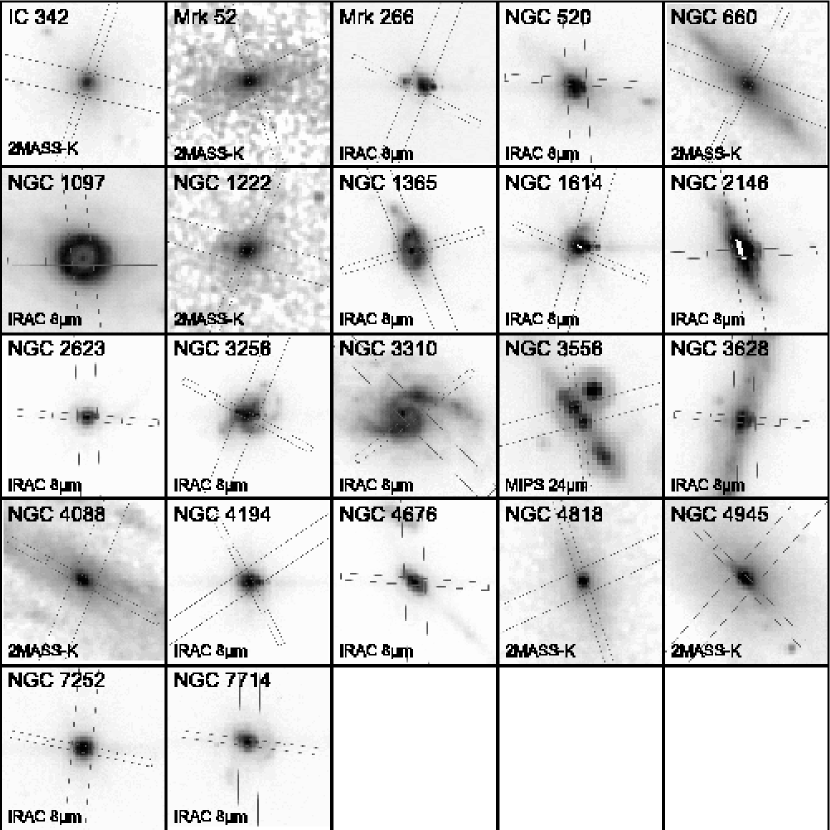
Figure 1.— The positions of the SL and LL slits for the given observing date overplotted on IRAC $8\mu$m, MIPS $24\mu$m or 2MASS K-band images for all galaxies in our sample. The scale is logarithmic and overemphasizes the real flux distribution. For discussion see section 2.3.

2.2. Data Reduction

The data were pre-processed by the Spitzer Science Center (SSC) data reduction pipeline version 11.0 (SOM, 2004) (except for NGC 3256, which was processed with version 12). To avoid uncertainties introduced by the flat-fielding in earlier versions of the automated pipeline processing we started from the two-dimensional, unflat-fielded data products, which only lack stray light correction and flat fielding. These products are part of the “basic calibrated data” (BCD) package provided by the SSC. The various steps of the data reduction followed a recipe that has been developed by the IRS Disks team and tested on a large amount of Galactic and extragalactic spectra.

We used the Spectral Modeling, Analysis, and Reduction Tool (SMART) version 5.5.1., developed by the IRS team (Higdon et al., 2004) to reduce and extract the spectra. First, we median-combined the images of the same order, same module and same nod position. Then we differenced the two apertures to subtract the “sky” background, which is mainly from zodiacal light emission. We have done so by subtracting the spatially offset first and second order slits from each other: SL1 from SL2 and vice versa for the SL (short wave, low resolution) module, and LL1 from LL2 and vice versa for the LL (long wave, low resolution) module. We note that this approach assumes that the emission from the target is not farther extended than the angular distance between the two corresponding subslits of $79^{\prime\prime}$ in SL.

We extracted the spectra using a column width which increases – like the instrumental point-spread function – linearly with wavelength. The extraction width is set to four pixels at the central wavelength of each subslit. The spectra were flat-fielded and flux calibrated by multiplication with the relative spectral response function (RSRF) using the IRS standard star $\alpha$-Lac for both low resolution modules. We built our RSRF by extracting the spectra of calibration stars (Cohen et al., 2003) in the same way as we perform on our sources, then divide the template spectra of those standard stars by the spectra we extracted with the column extraction method. Finally, we multiplied the spectra of the science target by the RSRF, for each nod position.

Figure 1 shows the positions of the narrower SL and wider LL slits for the given observing date overplotted on mid-IR images from IRAC, MIPS, and 2MASS in logarithmic scale. Our anticipated slit positions agree quite well with the main peak of the mid-IR emission, except for NGC 1097, NGC 3310, and NGC 3556, which show a more complex morphology. The consequences of slight mismatches and extended emission are discussed in the following section.

2.3. Absolute Fluxes and Order Stitching

After the spectral extraction there was, in some cases, a noticeable mismatch between the spectra from the different IRS modules. Since this mismatch is more likely due to source flux that was missed in the narrower slits rather than unrelated flux that was picked up in the wider slits (see below) we scaled the SL2, SL1, and LL2 spectra to match the flux density of LL1. The choice of LL1 as reference slit is appropriate because it has the widest slit and largest PSF, and is least sensitive to pointing errors or a small spatial extent of the mid-IR emission region. We have also used the “bonus orders” SL3 and LL3 when they provided better overlap or higher signal-to-noise than first and second orders only. The applied stitching factors are listed in Table 2 and provide a good idea of the uncertainties involved. Since these factors are rather large in some cases we would like to emphasize the rationale for this approach. The problem of stitching together slit apertures of different widths is by no means specific to our approach, but applies to basically all comparable studies at almost all wavelengths. For a black-body-like object with extended, uniform surface brightness there will be a jump between the SL slit width ($3.6^{\prime\prime}$) to the LL slit $10.5^{\prime\prime}$, corresponding to an increase in flux of at least a factor of three. Since all spectral energy distributions are continuous, scaling SL to match LL seems reasonable to first order.

However, this approach assumes that the spectral properties are not changing within the region covered by the LL slit, corresponding to linear scales of about 200 pc for the nearest objects in our sample – the typical size of a circum-nuclear starburst over which the spectral properties are assumed to not vary substantially. If the contributions from a centrally concentrated source, e.g., an AGN, were dominant, scaling would lead to an overestimation of the strength of the features originating in the center.

For the latter reason we have decided to list the flux densities as measured from the stitched spectra, but not to overall scale the IRS spectra to match the spatially integrated IRAS flux densities at $25\mu$m. We have calculated the $\nu f_{\nu}$ average of the IRS spectra over the $25\mu$m IRAS filter band. The ratio of IRS to IRAS $25\mu$m flux densities is given as the fractional flux ’FF’ in Table 2, last column. We note that color corrections applied to the published IRAS catalog fluxes increase the uncertainties, but the relative effect on our sample with similar SEDs is small. In some cases the ratio is quite small, indicating a rather large apparent discrepancy between IRS and IRAS. This is mainly due to two reasons: (i) the galaxy extends over a large angle and the mid-IR emission region is significantly more extended than the IRS slit (e.g., NGC 3628, NGC 4945), or (ii) the galaxy has significant off-nuclear IR emission peaks (e.g., NGC 3556, NGC 4088).

Figure 1 shows that substructure or extended emission on scales of the IRS slit is present in many of our objects, most notably in those which have small fractional fluxes ‘FF’ in Table 2. The most extreme cases are NGC 1097, NGC 3556, and NGC 4088. NGC 3556 shows a bright, off-nuclear mid-IR source and several IR-bright knots along the disk. NGC 4088 is very extended with IR emission in the disk that is picked up in the large IRAS beam. In the case of NGC 1097 it is clear from Figure 1 that the very symmetrical ring is the reason why we only see 21% of the flux. Although we do not scale our measured spectra to match the IRAS fluxes, the factor FF will become very important in section 4 where we use absolute fluxes to derive total luminosities and star formation rates.

All of the individual IRS spectra are shown in Fig. 2. We have not attempted to correct for the periodic “fringing” in the spectra longward of about $22\mu$m, which can be very prominent, as in NGC 1614. These artifacts have no effect on the analysis carried out in this paper.

Figure 2.— Spitzer-IRS low-resolution spectra of of all starburts in our sample on logartithmic scale. The most prominent spectral features (fine-structure lines, H₂ lines, PAHs and silicate features) are labeled. For absolute flux calibration see the discussion in section 2.3.

Fig. 2. cont’d —

Fig. 2. cont’d —

Fig. 2. cont’d —

Fig. 2. cont’d —

Fig. 2. cont’d —

3. Analysis

Figure 3 shows a normalized overlay of nine starburst spectra from our sample with the most prominant spectral features labeled. The figure illustrates the spectral richness of the $5-38\mu$m wavelength range and reveals distinct differences between individual starbursts. Important common features include PAH emission bands, silicate emission or absorption features, and emission lines, in addition to the information contained in the slope of the spectral continuum. In the following subsections we discuss how the quantities relevant to our discussion have been measured from our spectra.

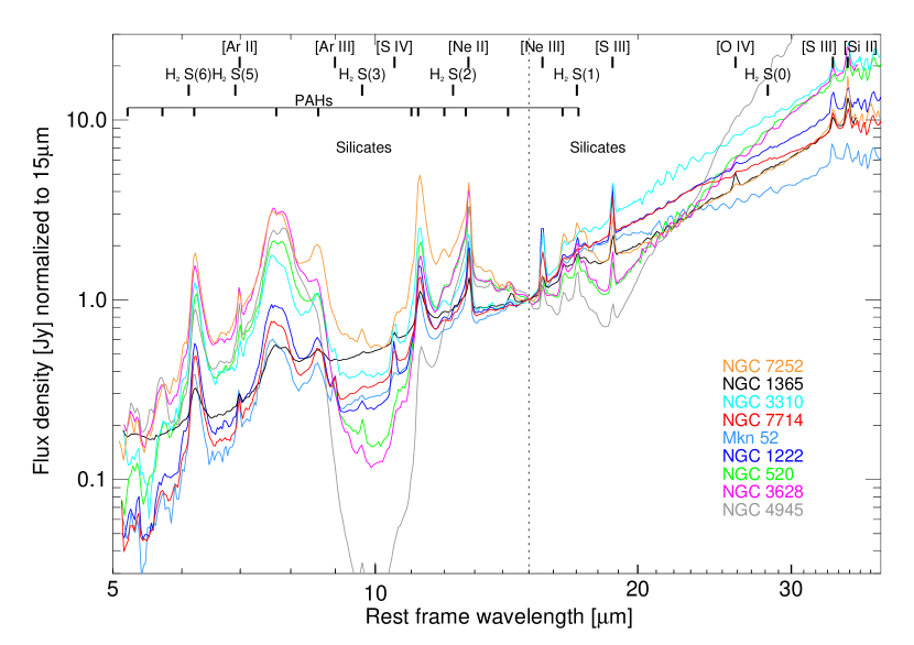
Figure 3.— Overlay of nine IRS starburst spectra of Mkn 52, NGC 520, NGC 1222, NGC 1365, NGC 3310, NGC 3628, NGC 4945, NGC 7252, and NGC 7714. The objects shown here have been selected to illustrate the full spectral diversity of starbursts with a small number of objects. All spectra have been normalized to a flux density of one at $15\mu$m (dotted vertical line).

3.1. Continuum Fluxes

In order to characterize the basic properties of the spectral continuum we have derived the flux densities for three rest frame wavelength ranges: at $5.9-6.1\mu$m, at $14.75-15.25\mu$m, and at $29.5-30.5\mu$m. These wavelengths were chosen to cover a large baseline in wavelength while being least affected by PAH emission features, silicate absorption or strong emission lines. The flux densities derived for $6\mu$m, $15\mu$m, and $30\mu$m are the median values in the above wavelength ranges, respectively, and are arguably the best direct estimate of the spectral continuum. The measured fluxes are listed in Table 3. In section 4.2 we will use these continuum fluxes to estimate the total luminosity of the starburst galaxy.

Table 3Continuum fluxes and extinction

Name	$F_{6\mu m}$	$F_{15\mu m}$	$F_{30\mu m}$	$\tau_{9.8}$
	[Jy]	[Jy]	[Jy]
IC 342	0.38	2.71	27.26	0.004
Mrk 52	0.03	0.28	1.19	-0.003
Mrk 266	0.03	0.17	1.16	0.373
NGC 520	0.15	0.54	6.12	0.994
NGC 660	0.34	1.27	11.52	1.293
NGC 1097	0.12	0.29	3.23	0.130
NGC 1222	0.06	0.38	3.03	0.213
NGC 1365	0.32	1.55	9.61	-0.034
NGC 1614	0.14	1.10	5.80	0.279
NGC 2146	0.74	2.00	23.07	0.845
NGC 2623	0.06	0.32	4.75	1.544
NGC 3256	0.34	2.36	21.61	0.000
NGC 3310	0.08	0.24	2.79	0.057
NGC 3556	0.02	0.10	1.10	0.230
NGC 3628	0.19	0.46	4.89	1.640
NGC 4088	0.04	0.12	0.76	0.307
NGC 4194	0.22	0.79	6.77	0.371
NGC 4676	0.03	0.07	0.45	0.580
NGC 4818	0.13	0.92	5.56	-0.160
NGC 4945	0.48	1.83	49.56	4.684
NGC 7252	0.06	0.11	0.69	-0.098
NGC 7714	0.07	0.53	3.48	-0.096

3.2. Polycyclic Aromatic Hydrocarbons (PAHs)

The spectra in Fig. 3 show that the spectral continuum shape of starburst spectra is dominated by strong emission features from PAHs (as previously noted by ISO authors, e.g., Genzel & Cesarsky (2000) and references therein). Although the first detections of PAHs date back in the 1970s, it took more than 10 years to identify them. Here we concentrate our analysis on several of the strongest PAH features at $6.2\mu$m, $7.7\mu$m, $8.6\mu$m, $11.3\mu$m, $14.2\mu$m, and around $17\mu$m (which is in fact two blended PAH complexes centered at $16.4\mu$m and $17.1\mu$m). Further PAH features can be seen in the spectra (see sections 3.5 and 4.6) but have either low S/N or are, at the low resolution of the IRS SL+LL modules, blended with other features and were thus excluded from this analysis. At the IRS low-resolution the $12.7\mu$m PAH blends with the strong [Ne II] line at $12.81\mu$m. This feature will be discussed by Devost et al. (2006) in the context of the IRS high resolution spectra.

The strengths of the $6.2\mu$m, $7.7\mu$m, $8.6\mu$m, and $11.3\mu$m PAH emission bands were derived by integrating the flux of the feature in the mean spectra of both nod positions above an adopted continuum. For the 6.2 and $11.3\mu$m features this baseline was determined by fitting a spline function to four or five data points. The wavelength limits for the integration of the features were approximately between 5.94 to $6.56\mu$m in the case of the $6.2\mu$m PAH and between 10.82 and $11.80\mu$m for the $11.2\mu$m PAH. For most spectra this method produced results, reproducable to within 5% for repeated fits with different choices of the continuum or integration limits to account for uncertainties within the fitting procedure. Only for the noisiest spectra this uncertainty increased to 15%. The baseline for the the $7.7\mu$m and $8.6\mu$m features was derived by fitting a spline through six data points avoiding small features in the range between 5.5 and $10\mu$m. Our method is illustrated in Figure 4. The selected data points for the baseline were chosen at the same wavelengths for all spectra. Following Peeters et al. (2002) we included one point close to $8.2\mu$m to separate the contribution from both features.

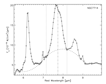
Figure 4.— Illustration of how the $7.7\mu$m PAH strength was measured in NGC 7714. The light grey dots represent the continuum points, interpolated by the dashed spline function. The vertical dotted lines indicate the integration range for the $7.7\mu$m feature.

The PAH features at $14.2\mu$m (Hony et al., 2001) and $17\mu$m (van Kerckhoven et al., 2000) are intrinsically weaker but are located in spectrally less complex regions, allowing a different approach. The strength of the $14.2\mu$m feature was determined through a first order baseline fit to the continuum at $13.88-14.03\mu$m and $14.54-14.74\mu$m. Similarly, the strength of the $17\mu$m complex was determined through a first order baseline fit to the continuum at $15.95-16.15\mu$m and $18.20-18.40\mu$m. We emphasize that the feature we refer to as the $17\mu$m PAH is in fact a blend of two PAH complexes at $16.4\mu$m and $17.1\mu$m. The latter is furthemore contaminated by the H₂S(1) line at $17.0\mu$m. The individual components of this complex cannot be properly resolved in the low-resolution spectra and we give only combined fluxes here. The equivalent widths for all features were derived by dividing the integrated PAH flux above the adopted continuum by the continuum flux density at the center of the feature (indicated by the vertical dot-dashed line in Figure 4). The derived PAH fluxes and equivalent widths are listed in Table 4.

Table 4Main PAH feature strengths shortward of $18\mu$m

	$6.2\mu$m PAH		$7.7\mu$m PAH		$8.6\mu$m PAH		$11.3\mu$m PAH		$14.2\mu$m PAH		$17\mu$m PAH
Name	Flux	EW	Flux	EW	Flux	EW	Flux	EW	Flux	EW	Flux	EW
IC342	14.65	0.497	31.75	0.581	7.39	0.168	18.36	0.492	0.50	0.014	9.70	0.178
Mrk52	1.07	0.535	2.14	0.552	0.51	0.151	1.02	0.316	0.02	0.005	0.66	0.142
Mrk266	0.59	0.619	0.92	0.467	0.00	0.126	0.47	0.422	0.08	0.065	0.51	0.403
NGC0520	5.60	0.563	13.97	0.528	1.99	0.126	5.62	0.798	0.20	0.024	2.91	0.494
NGC0660	12.91	0.504	27.36	0.518	3.81	0.123	9.72	0.701	0.43	0.023	6.26	0.365
NGC1097	5.04	0.459	9.30	0.488	2.26	0.168	5.34	0.661	0.12	0.021	3.82	0.523
NGC1222	2.17	0.624	4.64	0.606	0.79	0.130	2.56	0.566	0.08	0.015	1.47	0.231
NGC1365	2.74	0.111	6.37	0.213	1.30	0.045	4.60	0.180	0.62	0.029	5.59	0.250
NGC1614	13.05	0.561	24.67	0.514	5.01	0.138	9.77	0.379	—	—	5.10	0.154
NGC2146	22.22	0.545	58.26	0.643	10.51	0.175	21.53	0.829	1.20	0.044	13.60	0.492
NGC2623	1.83	0.598	4.00	0.454	0.76	0.131	1.28	0.527	0.01	0.002	0.71	0.205
NGC3256	8.02	0.603	17.60	0.533	3.03	0.123	8.52	0.471	0.71	0.040	8.12	0.205
NGC3310	3.35	0.789	5.38	0.591	1.16	0.178	2.98	0.748	0.07	0.022	1.08	0.229
NGC3556	1.22	0.502	2.92	0.523	0.51	0.135	1.52	0.811	0.06	0.039	0.84	0.542
NGC3628	7.45	0.500	19.72	0.588	1.59	0.095	4.14	0.797	0.25	0.034	3.45	0.684
NGC4088	1.17	0.496	2.43	0.483	0.51	0.130	1.27	0.603	0.05	0.025	0.97	0.509
NGC4194	7.09	0.529	14.67	0.578	3.06	0.165	6.31	0.590	0.25	0.022	3.10	0.241
NGC4676	1.05	0.610	2.15	0.551	0.44	0.192	0.97	0.812	0.04	0.038	0.52	0.590
NGC4818	4.06	0.459	9.56	0.555	1.84	0.123	4.39	0.344	0.05	0.004	2.43	0.151
NGC4945	12.13	0.432	40.34	0.490	0.13	0.003	3.55	0.558	0.50	0.024	5.37	0.519
NGC7252	2.09	0.585	4.48	0.549	1.06	0.176	2.95	0.931	0.04	0.024	1.35	0.792
NGC7714	2.67	0.601	5.62	0.642	1.06	0.135	2.79	0.394	0.04	0.006	1.05	0.114

It is important to note that the values in Table 4 have not been corrected for extinction. While in many sources the silicate absorption band around $9.8\mu$m is very weak, objects severely affected by extinction, like NGC 4945, show a strong $7.7\mu$m PAH but much weaker $8.6\mu$m and $11.3\mu$m features. The cause of these variations will be addressed in section 4.6.

We do not list uncertainties for the PAH strengths in Table 4. The statistical errors from the fits to the high S/N are small compared to other uncertainties such as: (i) The error in the absolute flux calibration of each module, which is currently about $5-10\%$. (ii) The error from scaling the individual orders for an extended source to match, as discussed in section 2.3. (iii) The error in the approximation of the underlying continuum, which is often dominated by strong, adjacent emission and absorption features and varies from source to source, and (iv) The error in the strength of the $17\mu$m PAH from the blending of two PAH complexes and the H₂S(1) line.

Our measurement procedures have been designed to minimize these errors as best as possible. The dominant error remains the uncertainty in the flux calibration, and we estimate the error in the PAH measurements to be in the order of $10\%$.

3.3. Emission Lines

The $5-38\mu$m wavelength range contains numerous strong emission lines. Among those are the following forbidden lines – sorted by wavelength and with their excitation potentials in parentheses:

[Ar II] $6.99\mu$m, [Ar III] $8.99\mu$m, [S IV] $10.51\mu$m, [Ne II] $12.81\mu$m, [Ne III] $15.56\mu$m, [S III] $18.71\mu$m, [O IV] $25.89\mu$m, [S III] $33.48\mu$m, and [Si II] $34.82\mu$m. In addition, we detect the pure rotational lines of molecular hydrogen H₂ (0,0) S(5) $6.91\mu$m (blended with [Ar II]), H₂ (0,0) S(3) $9.66\mu$m, H₂ (0,0) S(2) $12.28\mu$m, and H₂ (0,0) S(1) $17.03\mu$m.

All of these lines have been identified and labeled in Fig. 3. We list them here since they can be easily detected, even at $R\leq 100$. However, the flux measurements of the fine-structure lines can be done much more accurately from the IRS high-resolution spectra, which is the subject of a complementary paper discussing the ionic properties of the ISM (Devost et al., 2006).

3.4. Silicate Absorption and Optical Depth

The wavelength coverage of IRS is ideally suited for a detailed study of the strong vibrational resonances in the silicate mineral component of interstellar dust grains. Amorphous silicates — the most common form of silicates — have a broad Si–O stretching resonance peaking at $9.8\mu$m and an even broader O–Si–O bending mode resonance peaking at $18.5\mu$m.

We have estimated the apparent optical depth in the $9.8\mu$m silicate feature from the ratio of the local mid-infrared continuum to the observed flux at $9.8\mu$m. For shallow silicate features, the local continuum may be defined as an F_λ power law interpolation between continuum pivots at $5.5\mu$m (averaged $5.3-5.7\mu$m flux) and $14.5\mu$m (averaged $14.0-15.0\mu$m flux), thus avoiding the main PAH emission complexes at $6-9\mu$m and $11-13\mu$m.

For starburst spectra with a more pronounced silicate feature, the continuum in the $14-15\mu$m range is affected by weak absorption from the overlapping wings of the 9.8 and $18\mu$m silicate features. For these spectra we define a second local continuum, by replacing the continuum pivot at $14.5\mu$m by a continuum pivot at $28\mu$m (averaged $27.5-28.5\mu$m flux) and use the average of the optical depths derived with either local continuum as the best estimate of the apparent $9.8\mu$m silicate optical depth.

Most fluxes used in this analysis are observed flux densities. However, in Fig. 15 we correct the observed fluxes for extinction. To get an estimate of the uncertainties we use two extinction laws from Draine (1989) and Lutz (1999) and show the difference in Fig. 15. The relative silicate absorption values $A_{\lambda}/A_{V}$ for the relevant PAH wavelengths are listed in Table 5.

Table 5Relative absorption values interpolated from Draine (1989) and Lutz (1999)

Wavelength	$A_{\lambda}^{Draine}/A_{V}$	$A_{\lambda}^{Lutz}/A_{V}$
$6.2\mu$m	0.0164	0.0489
$7.7\mu$m	0.0112	0.0440
$9.8\mu$m	0.0554	0.1289
$11.3\mu$m	0.0375	0.0872

Some estimates of $\tau_{9.8\mu m}$ in Table 3 are negative, implying that silicates are observed in emission. However, the absolute values are quite small and may just represent uncertainties in our baseline definition (see section 4.3 for a discussion). We also note that the true silicate optical depth may be significantly larger than the apparent silicate optical depth if the emitting and absorbing sources are mixed along the line of sight; if part of the silicate column is warm; or if the absorption spectrum is diluted by unrelated foreground emission.

3.5. Spectral Features in the $5-8\mu$m Range

The $5-8\mu$m spectral range of starburst galaxies is extremely rich in atomic and molecular emission and absorption features, and dominated by emission from the $6.2\mu$m PAH feature and the blue wing of the $7.7\mu$m PAH complex. Weaker emission features are expected from atomic lines ([Fe II] at $5.34\mu$m and [Ar II] at $6.99\mu$m), molecular hydrogen (H₂ S(7) at $5.51\mu$m and H₂ S(5) at $6.91\mu$m), and ‘combination-mode’ PAH emission bands (at $5.25\mu$m and $5.70\mu$m). Absorption features of water ice and hydrocarbons, commonly detected in deeply obscured galactic nuclei (Spoon et al., 2002), would be expected at $6.0\mu$m (water ice) and $6.90\mu$m and $7.25\mu$m (C–H bending modes in aliphatic hydrocarbons).

As illustrated by the average starburst spectrum in Fig. 6, PAH combination-mode emission features are common in our starburst spectra. Inspection of the individual spectra shows that the $5.25\mu$m feature is usually double-peaked due to blending with the $5.34\mu$m [Fe II] line (e.g. NGC 1222 and NGC 3256). Likewise, the profile of the $5.70\mu$m PAH feature is affected by the presence of the H₂ S(7) line at $5.51\mu$m (most notably NGC 2623 and NGC 4945). The $5.70\mu$m PAH feature appears strongest in the spectrum of NGC 4945 (Fig. 5). The ratio of the $5.7\mu$m to $6.2\mu$m PAH in this source is 0.29, about 5 times higher than for most other starburst galaxies in our sample. Interestingly, the red wing of the $5.7\mu$m PAH feature coincides with the steep onset of the $6\mu$m water ice absorption feature, as illustrated in Fig. 5 by the steep change in slope at $5.7\mu$m in the spectrum of the ULIRG IRAS 20100–4156. Simple spectral modeling confirms that a screen of water ice absorption can indeed mimick a stronger $5.7\mu$m PAH feature by suppressing the red wing of the feature and the adjacent $5.9\mu$m continuum. The presence of water ice in the nucleus of NGC 4945 is further supported by the discovery of a $3\mu$m water ice absorption feature in the ISO–PHT–S and VLT–ISAAC spectra of the nucleus (Spoon et al., 2000). For the remaining galaxies in our sample, the $5-6\mu$m spectral structure does not provide evidence for the presence of water ice absorption. Hence, apart from NGC 4945, shielded cold molecular gas may not be as abundant in starburst nuclei as in ULIRG nuclei.

Figure 5.— Comparison of the average starburst template (dotted line) from Fig. 6 to the most extincted source within our sample, NGC 4945 (dashed line), and to the ULIRG IRAS 20100-4156 (solid line). The spectra are normalized at $5.7\mu$m. IRAS 20100-4156 has been chosen as a representative ULIRG from the sample of Spoon et al. (2006).

Absorption features of aliphatic hydrocarbons at 6.85 and $7.25\mu$m are thought to be tracers of the diffuse ISM (Chiar et al., 2000). These features are readily detected in the spectra of deeply obscured ULIRG nuclei such as IRAS 20100–4156 (Fig. 5). The average starburst spectrum (Fig. 6), in contrast, does not show similarly pronounced structure and the $7\mu$m range is dominated instead by the blend of $6.91\mu$m H₂ S(5) and $6.99\mu$m [Ar II]. However, individual starburst spectra show weak spectral structure in the $6.5-7.0\mu$m range. At $6.65\mu$m, a weak emission feature seems to be present, most notably in the spectra of IC 342, NGC 660, NGC 1614, NGC 2146, NGC 4088, NGC 4945 and NGC 7252. Peeters et al. (2002) identify this feature as a PAH emission band. The red wing of the $6.65\mu$m emission feature lies close to the expected onset of the $6.85\mu$m hydrocarbon absorption feature (Fig. 5). Especially in the spectrum of NGC 4945, the $6.5-7.0\mu$m spectral structure is consistent with the presence of hydrocarbon absorption at a strength of $\tau$(6.85 $\mu$m)=0.15$\pm$0.05 (Fig. 5). For other starburst galaxies the spectral structure is too shallow and/or the S/N of the spectra too low to identify hydrocarbon absorption with sufficient confidence.

Figure 6.— Average IRS spectrum of 13 starburst galaxies (IC 342, NGC 660, NGC 1097, NGC 1222, NGC 2146, NGC 3310, NGC 3556, NGC 4088, NGC 4194, NGC 4676, NGC 4818, NGC 7252, and NGC 7714). All spectra have been normalized to a flux density of one at $15\mu$m before co-addition. The dotted line shows the ISO-SWS spectrum of M82 (Sturm et al., 2000) for comparison.

3.6. The Starburst “Template Spectrum”

Although many spectral features show variations from one starburst galaxy to another, the magnitude of these changes is relatively small compared to the differences between different classes of objects, such as AGN, quasars, ULIRGs, or normal galaxies. It is common practice to classify objects in these categories, and the availability of reference spectra is of great interest. A reference “template” spectrum would allow a comparison how close a given spectrum is to a typical starburst galaxy or if it shows any atypical features. Furthermore, classifications of objects at high redshift often require fits to a library of template spectra.

We have constructed a high signal-to-noise “starburst template” from the spectra of IC 342, NGC 660, NGC 1097, NGC 1222, NGC 2146, NGC 3310, NGC 3556, NGC 4088, NGC 4194, NGC 4676, NGC 4818, NGC 7252, and NGC 7714. These are basically the objects from our sample with high fluxes and without a strong AGN component. The spectra have been normalized to a flux density of unity at $15\mu$m before averaging. Figure 6 shows the resulting “template spectrum” and Table 6 lists the “average” spectral properties derived from this composed spectrum.

Table 6Properties of the “average” starburst galaxy

Parameter	Value
$F_{6\mu m}$	26%
$F_{15\mu m}$	100%
$F_{30\mu m}$	856%
$6.2\mu$m PAH EW	$0.53\mu$m
$7.7\mu$m PAH EW	$0.53\mu$m
$8.6\mu$m PAH EW	$0.15\mu$m
$11.3\mu$m PAH EW	$0.66\mu$m
$14.2\mu$m PAH EW	$0.02\mu$m
$17\mu$m PAH EW	$0.36\mu$m
$\tau_{9.8}$	$0.24\pm 0.10$

Figure 6 also shows the ISO-SWS spectrum of M82 (Sturm et al., 2000), which is often being used as a starburst template, for comparison. Although the spectral slope longward of $15\mu$m is very similar, the two spectra show several distinct differences: the ISO-SWS spectrum of M82 does not show the pronounced PAH complex around $17\mu$m, it shows much stronger silicate absorption, and the flux density shortward of $12\mu$m is almost a factor of two lower that in our average starburst template. We provide the spectrum in ascii table format on our website.

4. Results and Discussion

It is important to keep in mind that the starburst spectra presented in this paper represent an entire starburst region, including numerous (super-)star clusters at various ages and evolutionary states, the surrounding PDRs which are internally and externally excited, and the warm and cold dust spread across the entire region as well as localized dust condensations. While many of the properties of local substructures are expected to vary significantly, the overall significance of these variations may be averaged out in the spatially integrated spectra. Our aim here is to search for global trends between the spectral properties derived in the previous section (silicate absorption features, PAH features, spectral continuum) and the global starburst properties ($L_{IR}$, radiation field).

4.1. The Continuum Slope as a SB/AGN Diagnostic

The slope of the mid-IR spectral continuum depends on the optical thickness, composition and temperature of graphite dust grains, which are related to the amount of silicate grains (Mathis, Rumpl & Nordsieck, 1977). The dominating species in the IRS spectral range are hot ($\geq 100$ K), large grains heated by ionizing, non-ionizing, and Ly$\alpha$ photons inside Hii  regions, and small ($\leq 100$ Å) grains heated by non-ionizing photons outside Hii  region (Mouri et al., 1997). In Fig. 7 we plot the continuum slope, parametrized by the ratio of the $15\mu$m and $30\mu$m flux densities versus the optical depth at $9.8\mu$m (section 3.4). The filled symbols in Fig. 7 (and all other figures thereafter) correspond to starbursts with a weak AGN component as identified in Table 1. Although not a tight correlation one can see the general trend that starbursts with stronger silicate absorption tend to have a steeper continuum at longer wavelengths.

Figure 7.— Optical depth at $9.8\mu$m versus the slope of the continuum as measured by the flux ratio of $15\mu$m to $30\mu$m. The filled diamonds correspond to starbursts with a weak AGN component. The dotted line is a linear fit to the data points. The highly obscured source NGC 4945 is not included in the fit..

The slope of the dust continuum depends on the energy distribution and spatial concentration of the heating source(s). Dale et al. (2000) found from ISOCAM data of 61 galaxies a $6.75\mu$m / $15\mu$m continuum slope near unity for more quiescent galaxies, whereas that ratio drops (i.e., the slope steepens) for galaxies with increased starburst activity. Furthermore, the continuum slope can serve as a discriminator between massive stars or an AGN as the underlying power source. This has already been known since IRAS (e.g., Wang (1992)), and was further refined in numerous papers based on ISOCAM observations. (See Genzel & Cesarsky (2000) for a more comprehensive overview). For instance, Laurent et al. (2000) studied the ISOCAM colors of a large variety of extragalactic objects revealing clear general trends between AGN, photo-dissociation region (PDR), and Hii  region dominated spectra. However, the characterization of an individual object often turns out to be difficult due to the intrinsically large scatter: the IRAS $12\mu$m filter includes the silicate absorption band as well as several PAH emission features and strong emission lines. The wavelength range covered by ISOCAM is limited to shorter wavelengths which are dominated by hot dust and a large variety of emission and absorption features (compare to Fig. 5).

Our narrowband continuum fluxes largely avoid these problems. Figure 8, analogous to a color-color diagram in stellar astronomy, shows the continuum flux ratios at $6\mu$m/$15\mu$m versus $15\mu$m/$30\mu$m. The total infrared luminosity $L_{IR}$ is represented by the size of the symbols. For comparison the figure also contains the classical AGN Cen A (Sy 2), I Zw 1 (Sy 1), Mrk 3 (Sy 2), NGC 1275 (Sy 2), NGC 4151 (Sy 1.5), and NGC 7469 (Sy 1.2) from Weedman et al. (2005). We also show the starburst-dominated ULIRGs IRAS 12112+0305, IRAS 22491-1808, and the AGN-dominated Mrk 231, Mrk 463, and Mrk 1014 from Armus et al. (2006b). NGC 6240 is a peculiar case with an intrinsic fractional AGN contribution to the bolometric luminosity of $~{}20-24\%$ (Armus et al., 2006a).

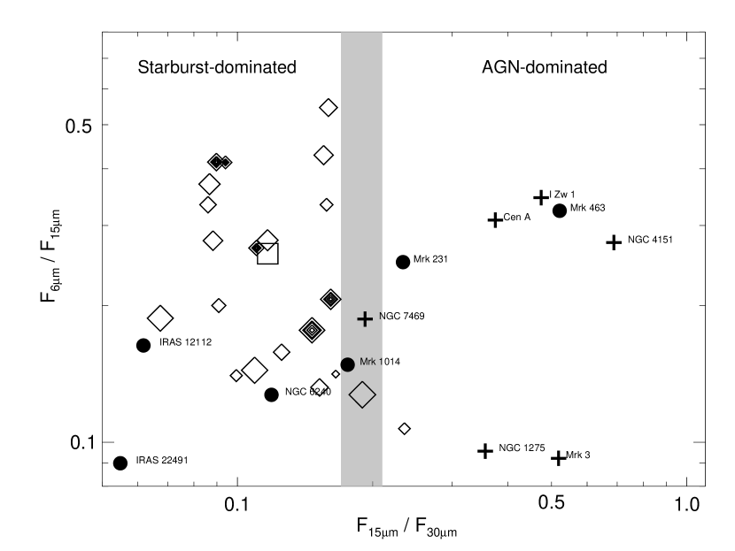
Figure 8.— “Color-color plot” of the $6\mu$m/$15\mu$m versus $15\mu$m/$30\mu$m flux densities. The size of the diamonds, representing our starburst sample, increases linearly with $\log L_{IR}$. The filled diamonds correspond to starbursts with a weak AGN component and the square refers to the average starburst template (Table 6). For comparison the figure also contains AGN (pluses) from Weedman et al. (2005), as well as ULIRGs (filled circles) from Armus et al. (2006a) and Armus et al. (2006b).

Several conclusions can be drawn from Fig. 8. First, there is a large scatter along the $y$-axis with no obvious correlation with total starburst luminosity or galaxy type. Hence, the $6\mu$m/$15\mu$m continuum flux ratio does not appear to be a good diagnostic. Second, using the $15\mu$m/$30\mu$m continuum flux ratio, classical (strong) AGN can be clearly separated from the starburst galaxies (including the ones with weak nuclear activity), with the AGN having a significantly shallower mid-IR spectrum. The grey-shaded bar in Fig. 8 indicates the transition region between AGN and starburst-dominated systems, and lies approximately at

$$0.17\leq F_{15\mu m}/F_{30\mu m}\leq 0.21.$$

Third, the difference in spectral slope also seems to apply to ULIRGs depending on their dominant power source. Hence, this technique may have a much broader application and should be verified with a much larger sample of different classes of objects.

4.2. The Continuum Fluxes as Measures of $L_{IR}$

The total infrared luminosity is an important parameter to estimate the energetics of a starburst and to characterize the underlying stellar population and rate of star formation. $L_{IR}$ is often derived from the four IRAS filter bands (Sanders & Mirabel, 1996). In this subsection we will check how accurately $L_{IR}$ can be derived from the two IRS continuum fluxes at $F_{15\mu m}$ and $F_{30\mu m}$ alone.

Numerous attempts to extrapolate $L_{IR}$ from one or two, mainly broad band fluxes can be found in the literature. Takeuchi et al. (2005) discuss various estimators of infrared luminosities, and find – for a very large sample of 1420 galaxies of different type – correlations of the form $\log L_{IR}=1.02+0.972\log L_{12\mu m}$, and $\log L_{IR}=2.01+0.878\log L_{25\mu m}$. Both $L_{12\mu m}$ and $L_{25\mu m}$ allow to predict $L_{IR}$ to an accuracy within a factor of $4-5$ at the 95% confidence level over a wide range in luminosities. These uncertainties are similar to the luminosities derived from the MIPS $24\mu$m flux alone for a large sample of SINGS galaxies (Dale et al., 2005). Chary & Elbaz (2001) found a similar relation fitting $15\mu$m ISO fluxes: $\log L_{IR}=(1.05\pm 0.174)+0.998\log L_{15\mu m}$. Förster Schreiber et al. (2004) found that the monochromatic $15\mu$m continuum emission is directly proportional to the ionizing photon luminosity, and hence the total infrared luminosity.

As discussed in section 4.1 the IRS fluxes $F_{15\mu m}$ and $F_{30\mu m}$ provide a rather accurate estimate of the “true” spectral continuum. In Figure 9 we plot a combination of $F_{15\mu m}$ and $F_{30\mu m}$ times $D^{2}$ versus the total infrared luminosity derived from the IRAS bands. Since the IRAS beam usually covers the entire starburst while the narrower IRS slits can only collect a fraction of the total luminosity for local starbursts (Fig. 1) we have corrected the observed $F_{15\mu m}$ and $F_{30\mu m}$ (indicated by the pluses in Fig. 9) for the slit losses (see section 2.3 for more details). A least-square fit to the corrected fluxes yields:

$$L_{IR}^{est}=D^{2}\cdot\left(4.27\cdot F_{15\mu m}+11\cdot F_{30\mu m}\right)$$

where $D$ is the distance in kiloparsecs, $F_{15\mu m}$ and $F_{30\mu m}$ the IRS flux densities in Janskies.

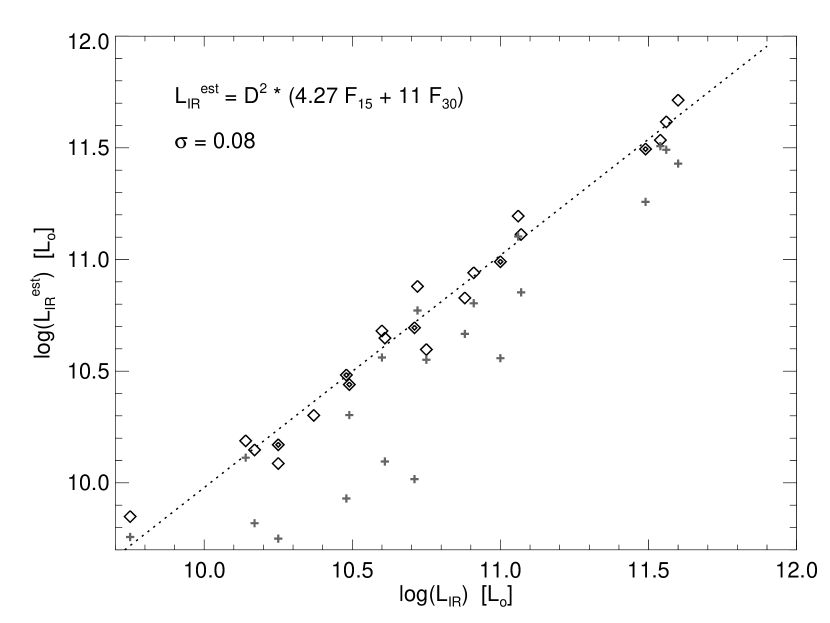
Figure 9.— The estimated infrared luminosity $L_{IR}^{est}$ based on the aperture loss corrected IRS continuum fluxes $F_{15\mu m}$ and $F_{30\mu m}$ for a source at distance $D$ [kpc] versus $L_{IR}$ from IRAS. The dashed line represents a linear fit to the data (in log-log space), and the fitted function is given in the upper left, together with the standard error $\sigma$. The uncorrected fluxes are indicated by gray plus signs. The filled symbols correspond to starbursts with a weak AGN component.

The correlation in Fig. 9 is extremely tight, including the weak AGN, with a standard error (mean scatter) of only 0.09 in log-space, i.e., the IRS estimated infrared luminosities agree within 23% with $L_{IR}$. This is much more accurate than the estimates by Chary & Elbaz (2001) and Takeuchi et al. (2005). The excellent correlation suggests that, at least for a homogeneous sample of starburst galaxies, $F_{15\mu m}$ and $F_{30\mu m}$ can be used to accurately derive $L_{IR}$.

4.3. A Large Variety in Silicate Absorption

Figure 10 shows, from top to bottom, a series of starburst spectra, sorted by increasing absorption of the $9.8\mu$m silicate resonance. Since the peak of the resonance coincides with a minimum between the $7-9\mu$m and $11-13\mu$m PAH emission complexes, the effect of silicate absorption only becomes apparent towards the lower half of the plot. Nevertheless, the figure strikingly illustrates the strong effect of amorphous silicates on the overall $5-38\mu$m spectral shape and the large variations even within one class of objects. Fig. 10 shows that the $10\mu$m trough can in fact become a dominating feature of the spectral shape of starbursts.

Figure 10.— The IRS spectra of Mkn 52, NGC 7714, NGC 1222, NGC 7252, NGC 2146, NGC 520, NGC 3628, and NGC 4945 arranged to illustrate the gradual effect of increasing silicate absorption from top to bottom. The flux densities $F_{\lambda}$ have been arbitrarily scaled for better comparision.

The top two spectra also show a broad emission structure beginning at about $16\mu$m and extending to $21-25\mu$m. The shape of this feature is consistent with that of an $18\mu$m silicate emission feature, which would make these the first detections of this feature in starburst galaxies. However, the emission structure could also be due to the C–C–C in-plane and out-of-plane bending modes of PAHs (van Kerckhoven et al., 2000). The identification of this feature will be discussed in a future paper. The remaining starburst galaxies in Fig. 10 do not show evidence for a similar emission structure. The $13-35\mu$m spectra, from NGC 1222 (top) to NGC 4945 at the bottom, show an increasingly pronounced depression, peaking at $18.5\mu$m, signalling increasingly strong silicate absorption. The latter result is in full agreement with the trend found for the $9.8\mu$m silicate feature.

Among all the galaxies classified as starbursts, NGC 4945 (bottom spectrum in Fig. 10) is a “special case” exhibiting by far the strongest dust obscuration to its nuclear region (Spoon et al., 2000). Based on the IRS spectrum, the apparent optical depth in the $9.8\mu$m silicate feature is at least four and may be higher, depending on the choice of the local continuum. Apart from strong amorphous silicate absorption, the line of sight also reveals the presence of a $23\mu$m absorption feature. Following the analysis of deeply obscured lines of sight towards ULIRG nuclei (Spoon et al., 2006), we attribute the $23\mu$m feature to crystalline silicates (forsterite). Their detection in NGC 4945 suggests that crystalline silicates are perhaps a more common component of the ISM and not just limited to ULIRG nuclei.

Figure 11 compares the average starburst template from Fig. 6 to NGC 4945, the most extincted source within our sample. For comparison we also show the heavily embedded ULIRG IRAS 08572+3915 from Spoon et al. (2006). The usually rather shallow $18\mu$m silicate band reduces the continuum by a large factor compared to the average starburst spectrum. While NGC 4945 has a similarly strong silicate absorption feature as the ULIRG IRAS 08572+3915, the starburst also shows strong PAH complexes near $16.4\mu$m and $17.1\mu$m, which are absent in the ULIRG spectrum. Crystalline silicates, causing the features at 16 and $19\mu$m in IRAS 08572+3915, appear to be absent in the starburst template, although they are more difficult to discern at our spectral resolution given the presence of PAH features and the [S III] line in that range.

Figure 11.— Comparison of the average starburst template (dotted line) from Fig. 6 to the most extincted source within our sample, NGC 4945 (dashed line), and to the ULIRG IRAS 08572+3915 (solid line), chosen as an extreme case of extinction from the sample of Spoon et al. (2006). The spectra have been normalized at $14.5\mu$m.

While NGC 4945 shows by far the most extreme silicate absorption within our sample it is not an exotic object but defines the endpoint of a sequence of increasing optical depths. Recently, Dale et al. (2006) reported on the Spitzer-SINGS survey of 75 nearby galaxies. The typical target in their sample shows only modest dust obscuration, consistent with an $A_{V}\sim 1$ foreground screen and a lack of dense clumps of highly obscured gas and dust. Unfortunately, we cannot distinguish between the local and global dust distributions. The differences may be due to evolutionary states, local geometries or other reasons. However, it is evident that starburst galaxies can have very little or large amounts of extinction, and the presence/absence of a strong dust feature is not a characteristic item.

4.4. The Mixture of PAHs and Dust

In this section we will investigate how the derived PAH strengths may depend on extinction within the starburst region. Table 4 already indicates that the relative fluxes of individual PAH features are not constant for different starbursts. Lu et al. (2003) have found a 25% spread in the ratio of the $11.3\mu$m / $7.7\mu$m PAH fluxes which they attribute to intrinsic galaxy-to-galaxy variations. However, extinction can affect the relative strength of features at different wavelengths by different amounts (Table 5). Rigopoulou et al. (1999) found that the dominant influence on the (ULIRG) PAH ratio is extinction, and that the $6.2\mu$m PAH gets suppressed relative to the $7.7\mu$m PAH for heavily dust extincted systems. In particular, the $8.6\mu$m and $11.3\mu$m PAH features lie at wavelengths that are heavily affected by silicate absorption.

Fig. 12 shows the $11.3\mu$m / $7.7\mu$m and $11.3\mu$m / $6.2\mu$m PAH flux ratios versus the apparent silicate optical depth $\tau_{9.8}$. A trend that starbursts with stronger dust absorption show relatively weaker $11.3\mu$m PAHs is evident. Fig. 12 suggests that extinction can affect the relative PAH strength in starbursts by up to a factor of about two.

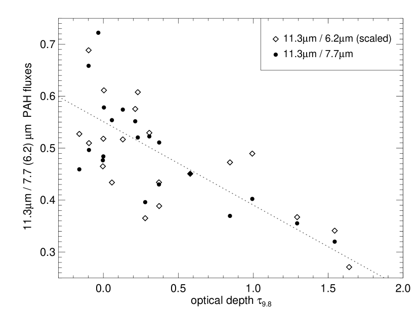
Figure 12.— The PAH flux ratios $11.3\mu$m/$7.7\mu$m (diamonds) and $11.3\mu$m/$6.2\mu$m (filled circles, divided by a factor 2.05 to match the other ratio) versus the optical depth at $9.8\mu$m, $\tau_{9.8}$ from Table 3. The dashed line shows a linear fit to both ratios but excluding NGC 4945.

In the remainder of this subsection we will investigate if the PAH equivalent width is related to the total infrared luminosity of the starburst. Rigopoulou et al. (1999) found a ratio of $L_{PAH}/L_{IR}$ which is similar for starburst-dominated ULIRGs and for template starbursts, i.e., no dependency on $L_{IR}$. In contrast, Lu et al. (2003) found a steady decrease of the PAH strength with increasing IR-activity. Figure 13 shows the equivalent widths of both the $6.2\mu$m and $7.7\mu$m PAH as a function of the total infrared luminosity for our starburst sample. Within the uncertainties, indicated by the scatter between the $6.2\mu$m and $7.7\mu$m PAHs for the same object, the PAH equivalent widths remain constant over a factor of 50 in total luminosity. This finding is in good agreement with Peeters et al. (2004) (and references therein) who found that the fraction of the total PAH flux emitted in the $6.2\mu$m PAH band varies only slightly with an average of $28\%\pm 4\%$. In other words, the PAH flux and the underlying warm dust continuum scale proportionally, and the PAHs and dust must be well mixed, at least on large scales, to show these correlations. This rules out a scenario of a luminous, dusty nucleus surrounded by a large PDR with little extinction, in favor of smaller, clumpier structures.

Figure 13.— The $6.2\mu$m (diamonds) and $7.7\mu$m (filled circles) PAH equivalent widths versus infrared luminosity $L_{IR}$. The dashed, horizontal line indicates a zeroth order polynomial fit to all data points, excluding the outlier NGC 1365. The filled diamonds correspond to starbursts with an AGN component.

4.5. PAH Luminosity and Star Formation Rate

Kennicutt (1998) has shown that the $8-1000\mu$m infrared luminosity $L_{IR}$ of starbursts is a good measure of the star formation rate (SFR) given by

$$\mbox{SFR}[M_{\odot}\mbox{yr}^{-1}]=4.5\times 10^{-44}L_{IR}[\mbox{erg\ s}^{-1}].$$

The SFR determines the number of young, massive stars, which provide the (far-)UV photons to excite both PAH molecules and dust grains. If both species get excited by the same photons PAHs could potentially be used as quantitative tracers of the SFR (see section 4.2 for the dust luminosity).

Generally, PAHs are considered the most efficient species for photoelectric heating (Bakes & Tielens, 1994) in the PDRs. Molecular gas in these boundary layers, surrounding the Hii  regions, is exposed to far-UV radiation ($6-13.6$ eV), which strongly influences its chemical and thermal structure (Tielens & Hollenbach, 1985). PAHs are stochastically heated by these UV photons, predominantly originating from massive stars, and hence expected to be good tracers of star formation. On large angular scales – similar to our case – Förster Schreiber et al. (2004) found that the $5-8.5\mu$m PAH emission constitutes an excellent indicator of the star formation rate in circumnuclear regions and starbursts as quantified by the Lyman continum flux, i.e. in regions where the energy output is dominated by massive star formation. However, it has been known for a long time that PAHS can also be excited by visible photons (e.g., Uchida et al. (1998)), and that PAHs can trace other sources besides massive young stars, such as planetary nebulae and reflection nebulae. If the observed PAH flux is integrated over the whole galaxy it may predominantly trace B stars, which dominate the Galactic stellar energy budget, rather than very recent massive star formation (Peeters et al., 2004). This is in agreement with higher angular resolution observations of the $3.3\mu$m PAH feature at the VLT by Tacconi-Garman et al. (2005), who found a decrease in the PAH/continuum ratio at the sites of the most recent star formation.

In section 4.4 we have seen that the PAH equivalent width does not dependent on $L_{IR}$. However, that does not necessarily mean that PAHs aren’t good quantitative tracers of star formation if the PAH feature and the underlying continuum scale proportionally. In Fig. 14 we compare the flux in the $6.2\mu$m PAH feature against the total infrared luminosity $L_{IR}$ from IRAS. To search for a physically meaningful correlation one needs to take the distance of the object into account as well as the fact that the narrow IRS slit misses some of the total flux. Hence we multiply the measured PAH fluxes with the square of the distances and divide by the fractional flux factor FF (Table 2). A remarkably good fit can been achieved with

$$\log\left(L_{IR}^{PAH}\right)=1.13\times\log\left(F_{6.2\mu mPAH}D^{2}\right)$$

where $F_{6.2\mu mPAH}$ is the $6.2\mu$m PAH flux in units of $10^{-19}\mbox{W\,cm}^{-2}$, $D$ the distance in kiloparsecs, and $L_{IR}$ in units of $L_{\odot}$. The standard error is 0.3 in $\log(L_{IR})$. Using the above equation, the total infrared luminosity of a starburst galaxy can be derived from the strength of a single PAH emission feature (here: the $6.2\mu$m PAH) to within a factor of two. This correlation is less tight than the estimate from the $F_{15\mu m}$ and $F_{30\mu m}$ continuum fluxes (section 4.2), supporting the finding by Peeters et al. (2004) that PAHs may not (only) trace recent massive star formation.

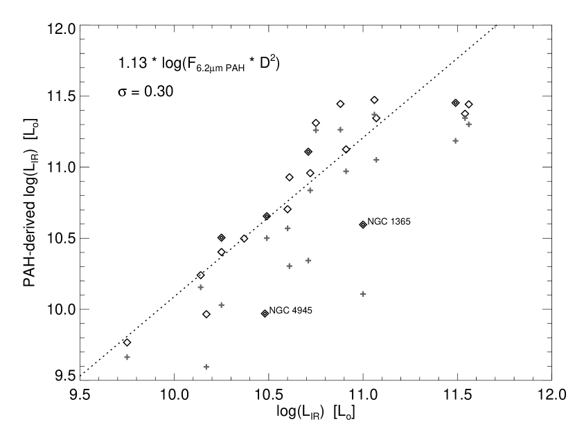
Figure 14.— The estimated infrared luminosity $L_{IR}^{PAH}$ based on the aperture corrected $6.2\mu$m PAH flux versus the total infrared luminosity as a measure of SFR. The gray plus signs refer to the location of the same data points if no aperture correction is applied. The dashed line represents a linear fit to the data (in log-log space), and the fitted function is given in the upper left, together with the standard error $\sigma$. The labeled outliers NGC 1365, NGC 4945 were excluded from the fit. The filled symbols correspond to starbursts with a weak AGN component.

Combining the information from Figs. 13 and 14 suggests that the continuum and the PAH emission are, to first order, proportional. Similarly, Peeters et al. (2004) have found that $L_{FIR}$ is proportional to the PAH luminosity $L_{6.2\mu m}$. If our spectra were “contaminated” by a significant amount of continuum emission from an AGN or an underlying, older galactic population unrelated to the starburst, the equivalent width would vary with distance (equivalent slit width), which is not observed. Hence, we conclude that both PAH and continuum emission originate predominantly from the starburst.

4.6. PAH Strength and Radiation Field

It is well known that the equivalent width of PAHs is much reduced in AGN-dominated environments (e.g., Sturm et al. (2000), Genzel & Cesarsky (2000), Weedman et al. (2005)). Geballe et al. (1989) have discussed the susceptibility of PAHs to destruction by far UV fields, and ISO observations (e.g., Cesarsky et al. (1996), Tran (1998)) have shown that more intense far-UV radiation fields may lead to gradual destruction of PAHs around stellar sources. Recently, Wu et al. (2006) studied a sample of low-metallicity blue compact dwarf galaxies from $1/50Z_{\odot}$ to $1/1.5Z_{\odot}$ with the IRS. They find a strong anti-correlation between strength (equivalent width) of the PAH features and the product of the [Ne III]/[Ne II] ratio (as a hardness measure of the radiation field) and the UV luminosity density devided by the metallicity. A similar trend has been reported by Madden et al. (2006) for a small sample of nearby dwarf galaxies. Unfortunately, lower metallicity and harder radiation fields seem to go hand-in-hand in these dwarf galaxies, and one cannot unambiguously distinguish between possibly suppressed PAH formation in low metallicity environments and PAH destruction in harder UV fields. Recently, Beirão et al. (2006) have investigated the strength of the $11.3\mu$m PAH feature in the starburst in NGC 5253 for different radial distances, and found that the equivalent width of the PAH feature is inversely proportional to the intensity of the radiation field, suggesting photo-destruction of the aromatic carriers in harsher environments.

Observations of Galactic sources (e.g., Verstraete et al. (1996), Vermeij et al. (2002)) have also shown that the relative strengths of individual PAH features can depend on the degree of ionization of the molecule: C-C stretching modes at $6.2\mu$m and $7.7\mu$m are stronger in ionized PAHs, while the C-H in-plane bending mode at $8.6\mu$m and the C-H out-of-plane bending mode at $11.3\mu$m are stronger by more than a factor of two in neutral PAHs. Comparing the ISOCAM spectra of M 82, NGC 253, and NGC 1808, Förster Schreiber et al. (2003) found that, while the $5-11\mu$m spectrum is nearly invariant, the relative PAH intensities exhibit significant variations of $20\%-100\%$, which they attributed to the PAH size distribution, ionization, dehydrogenation, or the incident radiation field.

In Fig. 15 we compare the ratio between the $11.3\mu$m bending mode and the $7.7\mu$m stretching mode to the hardness of the radiation field, as indicated by the [Ne III]/[Ne II] ratio from Devost et al. (2006), who provide a detailed analysis of the fine structure lines in our starburst sample. We correct both PAH fluxes for extinction (section 4.4) using the extinction laws by Draine (1989) and Lutz (1999) and the values from Table 5. Within the systematic uncertainties, represented by the scatter of the data points, we find no significant variation of the $7.7\mu$m / $11.3\mu$m PAH ratio over more than an order of magnitude in [Ne III]/[Ne II] fluxes. While we cannot exclude variations on scales of individual Hii  regions, our spatially averaged spectra of starburst nuclei do not reveal significant variations between the main PAH features. We have also looked at the weaker PAH features from Table 4, but the scatter increases with lower signal-to-noise and more uncertain baseline definition, and does not reveal an obvious trend. However, more studies, in particular of the PAH complex around $17\mu$m are planned.

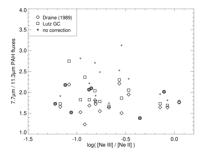
Figure 15.— The ratio of the $7.7\mu$m / $11.3\mu$m PAH fluxes versus the [Ne III]/[Ne II] line ratio (from Devost et al. (2006)). The PAH fluxes have been corrected for extinction using the laws from Draine (1989) (diamonds) and Lutz (1999) (squares). The gray pluses indicate the locations of the uncorrected values for reference. The filled diamonds correspond to starbursts with weak AGN components.

Our starburst sample spans a wide range in radiation field hardness. Fig. 16 shows the equivalent width of the $7.7\mu$m PAH feature versus the fine structure line ratio [Ne III]/[Ne II], which has been taken from Devost et al. (2006). Within the uncertainties the equivalent width of the $7.7\mu$m PAH feature remains constant over more than an order of magnitude in [Ne III]/[Ne II]. We conclude that, on large scales of starburst nuclei, which typically contain numerous Hii  regions, the PAH / continuum ratio does not significantly depend on the average radiation field hardness.

Figure 16.— The equivalent width of the $7.7\mu$m PAH feature versus the [Ne III]/[Ne II] line ratio (from Devost et al. (2006)) as an indicator of the hardness of the radiation field. The filled diamonds correspond to starbursts with weak AGN components. NGC 1365, which has a significant AGN component, is a clear outlier.

5. Summary

We presented and discussed the $5-38\mu$m mid-infrared spectra of a large sample of 22 starburst galaxies taken with the Infrared Spectrograph IRS on board the Spitzer Space Telescope. The high signal-to-noise spectra contain numerous important diagnostics such as PAH emission features, silicate bands at $9.8\mu$m and $18\mu$m, and the shape of the spectral continuum. The IRS spectral resolution of $R\approx 65-130$ is perfectly matched to study these features. From our sample we constructed an average starburst spectrum, which can be used as a starburst template.

The availability of continuous mid-infrared spectra of numerous objects within one class over a wide wavelength range enables various important studies. Remarkably, the spectra show a vast range in starburst SEDs. We found a trend that more dust extincted starburst systems have a steeper spectral continuum slope longward of $15\mu$m. The slope can also be used to discriminate between starburst and AGN powered sources, with a transition at $0.17\leq F_{15\mu m}/F_{30\mu m}\leq 0.21$. The monochromatic continuum fluxes, which represent a more accurate estimate of the “true” continuum than broad band filters, provide a remarkably accurate estimate of the total infrared luminosity via $L_{IR}^{est}=D^{2}\cdot(4.27\cdot F_{15\mu m}+11\cdot F_{30\mu m})$ (after correcting for slit losses for nearby, extended systems).

Our starburst spectra cover a wide range of silicate absorption depths, from essentially no absorption to heavily obscured systems with an optical depth of $\tau_{9.8\mu m}\sim 5$. We present the discovery of crystalline silicates in NGC 4945, which shows many similarities with heavily extincted ULIRGs. However, unlike the latter, the starbursts in our sample show no signs of water ices or hydrocarbons, suggesting a small amount of self-shielding.

The observed spectra show significant variations in the relative strengths of the individual PAH features at $6.2\mu$m, $7.7\mu$m, and $11.3\mu$m. However, these variations may be entirely due to extinction and do not necessarily indicate intrinsic variations of the PAH spectrum. We find that the PAH equivalent width is independent of the total luminosity $L_{IR}$, probably because the PAH strength and the underlying continuum scale proportionally within a “pure” starburst. The luminosity of an individual PAH feature, however, scales with $L_{IR}$. In particular the $6.2\mu$m feature can be used to approximate the total infrared luminosity of the starburst (although less accurately than from the $15\mu$m and $30\mu$m continuum fluxes).

We investigated possible variations of the PAH spectrum as expected, e.g., from varying degrees of PAH ionization. The $7.7\mu$m / $11.3\mu$m PAH ratios show no significant systematic variation with the hardness of the radiation field. Although our sample covers about a factor of ten difference in radiation field hardness (as indicated by the [Ne III] / [Ne II] ratio) we found no systematic correlation with the PAH equivalent width. Furthermore, we found no systematic differences between “pure” starbursts and galaxies with a weak, non-dominant AGN component for most of their spectral properties (except for NGC 1365 which shows very weak PAH emission).

We emphasize that these results are based on spatially integrated diagnostics over an entire starburst region. Local variations of age, IMF, density or geometry on the scales of individual Hii  regions or super star clusters may just average out. However, it is important to note that, because of this “averaging out effect” in unresolved sources, starburst nuclei with significantly different global properties may appear as rather similar members of one class of objects.

References

- Alonso-Herrero et al. (2001) Alonso-Herrero, A., Engelbracht, C.W., Rieke, M. J., Rieke, G.H., Quillen, A.C., 2001, ApJ, 546, 952
- Armus et al. (2006a) Armus, L., Bernard-Salas, J., Spoon, H.W.W., Marshall, J.A., Charmandaris, V., Higdon, S.J.U., Desai, V., Hao, L., Teplitz, H.I., Devost, D., Brandl, B.R., Soifer, B.T., Houck, J.R., 2006a, ApJ, 640, 204
- Armus et al. (2006b) Armus, L., et al., 2006b, submitted to ApJ
- Ashby et al. (1995) Ashby, M.L.N., Houck, J. R. & Matthews, K., 1995, ApJ, 447, 545
- Bakes & Tielens (1994) Bakes, E.L.O. & Tielens, A.G.G.M., 1994, ApJ427, 822
- Balzano (1983) Balzano, V. A., 1983, ApJ, 268, 602
- Bendo & Joseph (2004) Bendo, G.J. & Joseph, R.D., 2004, AJ 127, 3338
- Beirão et al. (2006) Beirão, P., Brandl, B., Devost, D., Smith, J.D., Hao, L., Houck, J.R., 2006, ApJ, accepted
- Beswick et al. (2003) Beswick, R. J., Pedlar, A., Clemens, M.S. & Alexander, P., 2003, MNRAS, 346, 424
- Brandl et al. (2004) Brandl, B. R., et al., 2004, ApJS, 154, 188
- Cesarsky et al. (1996) Cesarsky, D., Lequeux, J., Abergel, A., Perault, M., Palazzi, E., Madden, S., Tran, D., 1996, A&A, 315, 309
- Charmandaris et al. (2001) Charmandaris, V., Laurent, O., Mirabel, I.F., Gallais, P., 2001, ApSSS, 277, 55
- Chary & Elbaz (2001) Chary, R. & Elbaz, D., 2001, ApJ, 556, 562
- Chiar et al. (2000) Chiar, J.E., Tielens, A.G.G.M., Whittet, D.C.B., Schutte, W.A., Boogert, A.C.A., Lutz, D., van Dishoeck, E.F., Bernstein, M.P., 2000, ApJ, 537, 749
- Cohen et al. (2003) Cohen, M., Megeath, T.G., Hammersley, P.L., Martin-Luis, F. & Stauffer, J., 2003, AJ, 125, 2645
- Dale et al. (2000) Dale, D.A., Silbermann, N.A., Helou, G., Valjavec, E., Malhotra, S., Beichman, Ch.A., Brauher, J., Contursi, A., Dinerstein, H.L., Hollenbach, D.J. Hunter, D.A., Kolhatkar, S., Lo, K-Y., Lord, S.D., Lu, N.Y., Rubin, R.H., Stacey, G.J., Thronson, H.A., Jr., Werner, M.W., Corwin, H.G., Jr., 2000, AJ, 120, 583
- Dale et al. (2005) Dale, D.A., Bendo, G.J., Engelbracht, C.W., Gordon, K.D., Regan, M.W., Armus, L., Cannon, J.M., Calzetti, D., Draine, B.T., Helou, G., et al. 2005, ApJ, 633, 857
- Dale et al. (2006) Dale, D.A., Smith, J.D.T., Armus, L., Buckalew, B.A., Helou, G., Kennicutt, R.C., Moustakas, J., Roussel, H., Sheth, K., Bendo, G.J., Calzetti, D., Draine, B.T., Engelbracht, C.W., Gordon, K.D., Hollenbach, D.J., Jarrett, T.H., Kewley, L.J., Leitherer, C., Li, A., Malhotra, S., Murphy, E.J., Walter, F., 2006, ApJ, accepted
- Devost et al. (2006) Devost, D. et al., 2006, ApJ, in preparation
- Deveraux (1989) Deveraux, N. A., 1989, ApJ, 346, 126
- Draine (1989) Draine, B.T., 1989, Proceedings of the 22nd Eslab Symposium, ed. B.H. Kaldeich, ESA SP-290, 93
- Draine & Li (2001) Draine, B. T. & Li, A., 2001, ApJ, 551, 807
- Förster Schreiber et al. (2003) Förster Schreiber, Sauvage, M.,Charmandaris, V., Laurent, O., Gallais, P., Mirabel, I.F., Vigroux, L., 2003, A&A, 399, 833
- Förster Schreiber et al. (2004) Förster Schreiber, N.M., Roussel, H., Sauvage, M., & Charmandaris, V., 2004, A&A, 419, 501
- Fritze-v. Alvensleben & Gerhard (1994) Fritze-v. Alvensleben, U., Gerhard, O. E., 1994, A&A, 285, 775
- Gao & Solomon (2004) Gao, Y. & Solomon, P. M., 2004, ApJ, 606, 271
- Geballe et al. (1989) Geballe, T.R., Tielens, A.G.G.M., Allamandola, L.J., Moorhouse, A., Brand, P.W.J.L., 1989, ApJ, 341, 278
- Genzel & Cesarsky (2000) Genzel, R. & Cesarsky, C. J., 2000, ARA&A, 38, 761
- González-Delgado et al. (1999) González-Delgado, R. M., García-Vargas, M. L., Goldader, J., Leitherer, C. & Pasquali, A., 1999, ApJ, 513, 707
- Heckman et al. (1998) Heckman, T. M., Robert, C., Leitherer, C, Garnett, D. R. & van der Rydt, F., 1998, ApJ, 503, 646
- Helou et al. (2000) Helou, G., Lu, N.Y., Werner, M.W., Malhotra, S., Silbermann, N., 2000, ApJ, L21
- Higdon et al. (2004) Higdon, S.J.U., Devost, D., Higdon, J.L., Brandl, B.R., Houck, J.R., Hall, P., Barry, D., Charmandaris, V., Smith, J.D.T., Sloan, G.C., Green, J., 2004, PASP, 116, 975
- Ho et al. (1997) Ho, L. C., Filippenko, A. V., & Sargent, W.L.W., 1997, ApJS, 112, 315
- Hony et al. (2001) Hony, S., Van Kerckhoven, C., Peeters, E., Tielens, A.G.G.M., Hudgins, D.M., Allamandola, L.J., 2001, A&A, 370, 1030
- Houck et al. (2004) Houck, J. R. et al., 2004, ApJS, 154, 18
- Iwasawa et al. (1993) Iwasawa, K., Koyama, K., Awaki, H., Kunieda, H., Makishima, K., Tsuru, T., Ohashi, T. & Nakai, N., 1993, ApJ, 409, 155
- Joseph & Wright (1985) Joseph, R. D. & Wright, G. S., 1985, MNRAS, 214, 87
- Keel (1984) Keel, W. C., 1984, ApJ, 282, 75
- Kennicutt (1998) Kennicutt, R.C., 1998, ARA&A, 36, 189
- van Kerckhoven et al. (2000) Van Kerckhoven, C., Hony, S., Peeters, E., Tielens, A.G.G.M., Allamandola, L.J., Hudgins, D.M., Cox, P., Roelfsema, P.R., Voors, R.H.M., Waelkens, C., Waters, L.B.F.M., Wesselius, P.R., 2000, A&A, 357, 1013
- Keto et al. (1992) Keto, E., Ball, R., Arens, J., Jernigan, G., Meixner, M., 1992, ApJ, 389, 223
- Laurent et al. (2000) Laurent, O., Mirabel, I.F., Charmandaris, V., Gallais, P., Madden, S.C., Sauvage, M., Vigroux, L., Cesarsky, C., 2000, A&A, 359, 887
- Levenson et al. (2001) Levenson, N. A., Weaver, K. A. & Heckman, T. M., 2001, ApJS, 133, 269
- Liu & Kennicutt (1995) Liu, C. T. & Kennicutt, R. T. Jr., 1995, ApJ, 450, 547
- Lonsdale et al. (1984) Lonsdale, C. J., Persson, S. E. & Matthews, K., 1984, ApJ, 287, 95
- Lu et al. (2003) Lu, N., Helou, G., Werner, M.W., Dinerstein, H.L., Dale, D.A., Silbermann, N.A., Malhotra, S., Beichman, Ch.A., Jarrett, Th.H., 2003, ApJ, 588, 199
- Lutz et al. (1998) Lutz, D., Kunze, D., Spoon, H.W.W., Thornley, M.D., 1998, A&A, 333, 75
- Lutz (1999) Lutz, D., 1999, in The Universe as seen by ISO, Paris, Oct. 1998, ESA SP-427, 623
- Madden et al. (2006) Madden, S.C., Galliano, F., Jones, A.P., Sauvage, M., A&A, 446, 877
- Mathis, Rumpl & Nordsieck (1977) Mathis, Rumpl & Nordsieck, 1977, ApJ, 217, 425
- Mayya et al. (2004) Mayya, Y. D., Bressan, A., Rodriguez, M., Valdes, J. R. & Chavez, M., 2004, ApJ, 600,188
- Miller et al. (1997) Miller, B. W., Whitmore, B. C., Schweizer, F. & Fall, S. M., 1997, AJ, 114, 2381
- Mouri et al. (1997) Mouri, H., Kawara, K. & Taniguchi, Y. 1997, ApJ, 484, 222
- Osmer et al. (1974) Osmer, P. S., Smith, M. G. & Weedman, D. W., 1974, ApJ, 192, 279
- Osterbrock & Dahari (1983) Osterbrock, D. E. & Dahari, O., 1983, ApJ, 273, 478
- Peeters et al. (2002) Peeters, E., Hony, S., Van Kerckhoven, C., Tielens, A.G.G.M., Allamandola, L.J., Hudgins, D.M., Bauschlicher, C.W., 2002, A&A, 390, 1089
- Peeters et al. (2004) Peeters, E., Spoon, H.W.W. & Tielens, A.G.G.M., 2004, ApJ, 613, 986
- Rigby & Rieke (2004) Rigby, J. R. & Rieke, G. H., 2004, ApJ, 606, 237
- Rigopoulou et al. (1996) Rigopoulou, D., Lutz, D., Genzel, R., Egami, E., Kunze, D., Sturm, E., Feuchtgruber, H., Schaeidt, S., Bauer, O.H., Sternberg, A., Netzer, H., Moorwood, A.F.M., de Graauw, T., 1996, A&A, 315, L125
- Rigopoulou et al. (1999) Rigopoulou, D., Spoon, H.W.W., Genzel, R., Lutz, D., Moorwood, A.F.M., Tran, Q.D., 1999, AJ, 118, 2625
- Roberts et al. (2004) Roberts, T. P., Warwick, R. S., Ward, M. J. & Goad, M. R., 2004, MNRAS, 349, 1193
- Roche & Aitken (1985) Roche, P.F. & Aitken, D.K., 1985, MNRAS, 215, 425
- Sanders & Mirabel (1996) Sanders, D. B. & Mirabel, I.F., 1996, ARA&A, 34, 749
- Sanders et al. (2003) Sanders, D. B., Mazzarella, J. M., Kim, D.-C., Surace, J. A. & Soifer, B. T., 2003, AJ, 126, 1607
- Smith et al. (1998) Smith, D.A., Herter, T. & Haynes, M. P., 1998, ApJ, 494, 150
-
SOM (2004)
Spitzer Observer’s Manual, 2004,
http://ssc.spitzer.caltech.edu/documents/SOM/ - Spoon et al. (2000) Spoon, H.W.W., Koornneef, J., Moorwood, A.F.M., Lutz, D., Tielens, 2000, A&A, 357, 898
- Spoon et al. (2002) Spoon, H.W.W., Keane, J.V., Tielens, A.G.G.M., Lutz, D., Moorwood, A.F.M., 2001, A&A, 365, 353
- Spoon et al. (2006) Spoon, H.W.W., Tielens, A.G.G.M., Armus, L., Sloan, G.C., Sargent, B., Cami, J., Charmandaris, V., Houck, J.R., Soifer, B.T., 2006, ApJ, 638, 759
- Sternberg & Dalgarno (1989) Sternberg, A. & Dalgarno, A., 1989, ApJ, 338, 197
- Storchi-Bergmann et al. (2003) Storchi-Bergmann, T., Nemmen, R., Eracleous, M., Halpern, J. P., Filippenko, A. V., Ruiz, M. T., Smith, R. C. & Nagar, M., 2003, ApJ, 598, 956
- Sturm et al. (2000) Sturm, E., Lutz, D., Tran, D., Feuchtgruber, H., Genzel, R., Kunze, D., Moorwood, A.F.M., Thornley, M.D., 2000, A&A358, 481
- Tacconi-Garman et al. (2005) Tacconi-Garman, L.E., Sturm, E., Lehnert, M., Lutz, D., Davies, R.I., Moorwood, A.F.M., 2005, A&A, 432, 91
- Takeuchi et al. (2005) Takeuchi, T.T., Buat, V., Iglesias-Paramo, J., Boselli, A., Burgarella, D., 2005, A&A, in press
- Thornley et al. (2000) Thornley, M. D., Schreiber, N. M. F., Lutz, D., Genzel, R., Spoon, H. W. W., Kunze, D. & Sternberg, A., 2000, ApJ, 539, 641.
- Tielens & Hollenbach (1985) Tielens, A. G. G. M. & Hollenbach, 1985, ApJ, 291, 722
- Tran (1998) Tran, Q.D., 1998, Ph.D. Thesis, Université de Paris XI
- Uchida et al. (1998) Uchida, K.I., Sellgren, K., & Werner, M.W., 1998, ApJ, 493, L109
- Verma et al. (2003) Verma, A., Lutz, D., Sturm, E., Sternberg, A., Genzel, R. & Vacca, W., 2003, A&A, 403, 829
- Vermeij et al. (2002) Vermeij, R., Peeters, E., Tielens, A.G.G.M., van der Hust, J.M., 2002, A&A, 382, 1042
- Veron et al. (1980) Veron, P., Lindblad, P.O., Zuiderwijk, E.J., Veron, M.P. & Adam, G., 1980, A&A, 87, 245
- Verstraete et al. (1996) Verstraete, L., Puget, J.L., Falgarone, E., Drapatz, S., Wright, C.M., Timmermann, R., 1996, A&A, 315, 337
- Wang (1992) Wang, G., 1992, AcApS, 11, 311
- Weedman et al. (1981) Weedman, D. W., Feldman, F. R., Balzano, V. A., Ramsey, L. W., Sramek, R. A. & Wu, C.-C., 1981, ApJ, 248, 105
- Weedman et al. (2005) Weedman, D.W., Hao, L., Higdon, S.J.U., Devost. D., Wu, Y., Charmandaris, V., Brandl, B.R., Armus, L., Spoon, H.W.W., Bass, E., Houck, J.R., 2005, ApJ, accepted
- Werner et al. (2004) Werner, M. et al., 2004, ApJS, 154, 1
- Wu et al. (2006) Wu, Y., Charmandaris, V., Hao, L., Brandl, B.R., Bernard-Salas, J., Spoon, H.W.W., Houck, J.R., 2005, ApJ, 639, 157