Static and Dynamic Modeling of a Solar Active Region. I: Soft X-Ray Emission

Abstract

Recent simulations of solar active regions have shown that it is possible to reproduce both the total intensity and the general morphology of the high temperature emission observed at soft X-ray wavelengths using static heating models. There is ample observational evidence, however, that the solar corona is highly variable, indicating a significant role for dynamical processes in coronal heating. Because they are computationally demanding, full hydrodynamic simulations of solar active regions have not been considered previously. In this paper we make first application of an impulsive heating model to the simulation of an entire active region, AR8156 observed on 1998 February 16. We model this region by coupling potential field extrapolations to full solutions of the time-dependent hydrodynamic loop equations. To make the problem more tractable we begin with a static heating model that reproduces the emission observed in 4 different Yohkoh Soft X-Ray Telescope (SXT) filters and consider dynamical heating scenarios that yield time-averaged SXT intensities that are consistent with the static case. We find that it is possible to reproduce the total observed soft X-ray emission in all of the SXT filters with a dynamical heating model, indicating that nanoflare heating is consistent with the observational properties of the high temperature solar corona.

1 Introduction

Understanding how the Sun’s corona is heated to high temperatures remains one of the most significant challenges in solar physics. Unfortunately, the complexity of the solar atmosphere, with its many disparate spatial and temporal scales, makes it impossible to represent with a single, all encompassing model. Instead we need to break the problem up into smaller, more manageable pieces (e.g., see the recent review by Klimchuk 2006). For example, kinetic theory or generalized MHD is used to describe the microphysics of the energy release process. Ideal and resistive MHD are used to study the evolution of coronal magnetic fields and the conditions that give rise to energy release. Finally, one dimensional hydrodynamical modeling is employed to calculate the response of the solar atmosphere to the release of energy.

This last step is a critical one in the process of understanding coronal emission because it links theoretical models with solar observations. Even here, however, most previous work has focused on modeling small pieces of the Sun, such as individual loops (e.g., Aschwanden et al., 2001; Reale & Peres, 2000). Though understanding the heating in individual structures is an important first step, it has been difficult to apply this information to constrain the properties of the global coronal heating mechanism.

Recent advances in high performance computing have made it possible to simulate large regions of the corona, at least with static heating models. Schrijver et al. (2004), for example, have coupled potential field source-surface models of the coronal magnetic field with parametric fits to solutions of the hydrostatic loop equations to calculate visualizations of the full Sun. Comparisons between the simulation results and full-disk solar images indicate that the energy flux ($F_{H}$) into a corona loop scales as $B_{F}/L$, where $B_{F}$ is the foot point field strength and $L$ is the loop length. Schrijver & Title (2005) also find that this form for the heating flux is consistent with the flux-luminosity relationship derived from X-ray observations of other cool dwarf stars Schrijver & Title (2005).

Warren & Winebarger (2006) have performed similar simulations for 26 solar active regions using potential field extrapolations and full solutions to the hydrostatic loop equations. These simulation results indicate that the observed emission is consistent with a volumetric heating rate ($\epsilon_{S}$) that scales as $\bar{B}/L$, where $\bar{B}$ is the field strength averaged along the field line. In the sample of active regions used in that study $\bar{B}\sim B_{F}/L$ so that $F_{H}\sim\epsilon_{S}L\sim\bar{B}\sim B_{F}/L$, and this form for the volumetric heating rate is consistent with the energy flux determined by Schrijver et al. (2004).

In these previous studies it was possible to use static heating models to reproduce the high temperature emission observed at soft X-ray wavelengths, but not the lower temperature emission typically observed in the EUV. The static models are not able to account for the EUV loops evident in the solar images. Recent work has shown that the active region loops observed at these lower temperatures are often evolving (Ugarte-Urra et al., 2006; Winebarger et al., 2003). Simulation results suggest that these loops can be understood using dynamical models where the loops are heated impulsively and are cooling (e.g., Spadaro et al., 2003; Warren et al., 2003). Furthermore, spectrally resolved observations have indicated pervasive red shifts in active regions at upper transition region temperatures (e.g., Winebarger et al., 2002), suggesting that much of the plasma in solar active regions near 1 MK has been heated to higher temperatures and is cooling. Finally, Warren & Winebarger (2006) found that static heating in loops with constant cross section yields footpoint emission that is much brighter than what is observed. This suggests that static heating models may not be consistent with the observations, even in the central cores of active regions.

The need for exploring dynamical heating models of the solar corona is clear, but there are a number of problems that make this difficult in practice. One problem is the many free parameters possible in parameterizations of impulsive heating models. In addition to the magnitude and spatial location of the heating, it is possible to vary the temporal envelope and repetition rate of the heating (e.g., Patsourakos & Klimchuk, 2006; Testa et al., 2005). Furthermore, dynamical solutions to the hydrodynamic loop equations are much more computationally intensive to calculate than static solutions, limiting our ability to explore parameter space.

In this paper we explore the application of impulsive heating models to the high temperature emission observed in active region 8156 on 1998 February 16. To make the problem more tractable we begin with a static heating model that reproduces the emission observed in 4 different Yohkoh Soft X-Ray Telescope (SXT) filters and look for dynamical models that yield time-averaged SXT intensities that are in agreement with those computed from the static solutions. Relating the time-averaged intensities derived from the full dynamical solutions to the observed intensities is based on the idea that the emission from a single feature results from the superposition of even finer, dynamical structures that are in various stages of heating and cooling. This idea is similar to the nanoflare model of coronal heating (e.g., Parker, 1983; Cargill, 1994). Other nanoflare heating scenarios are possible, such as heating events on larger scale threads that are distributed randomly in space and time, but are not considered here. We find that it is possible to construct a dynamical heating model that reproduces the total soft X-ray emission in each SXT filter. This indicates that nanoflare heating is consistent with the observational properties of the high temperature corona.

2 Observations

Observations from SXT (Tsuneta et al., 1991) on Yohkoh form the basis for this work. The SXT, which operated from late 1991 to late 2001, was a grazing incidence telescope with a nominal spatial resolution of about 5″ (2$\farcs$5 pixels). Temperature discrimination was achieved through the use of several focal plane filters. The SXT response extended from approximately 3 Å to approximately 40 Å and the instrument was sensitive to plasma above about 2 MK.

In addition to the SXT images we use full-Sun magnetograms taken with the MDI instrument (Scherrer et al., 1995) on SOHO to provide information on the distribution of photospheric magnetic fields. The spatial resolution of the MDI magnetograms is comparable to the spatial resolution of EIT and SXT. In this study we use the synoptic MDI magnetograms which are taken every 96 minutes.

To constrain the static heating model we require observations of an active region in multiple SXT filters. Observations in the thickest SXT analysis filters, the “thick aluminum” (Al12) and the “beryllium” (Be119), are crucial for this work. As we will show, observations in the thinner analysis filters, such as the “thin aluminum” (Al.1) and the “sandwich” (AlMg) filters, do not have the requisite temperature discrimination for this modeling. To identify candidate observations we made a list of all SXT partial-frame (as opposed to full disk) observations with observations in the Al.1, AlMg, Al12, and Be119 filters between the beginning of the Yohkoh mission and the end of 2001. Since the potential field extrapolation is also important to this analysis, we required that the active lie within 400″ of disk center.

We also use consider observations from the EIT (Delaboudinière et al., 1995) on SOHO. EIT is a normal incidence telescope that takes full-Sun images in four wavelength ranges, 304 Å (which is generally dominated by emission from He II), 171 Å (Fe IX and Fe X), 195 Å (Fe XII), and 284 Å (Fe XV). EIT has a spatial resolution of 2$\farcs$6. Images in all four wavelengths are typically taken 4 times a day and these synoptic data are used in this study.

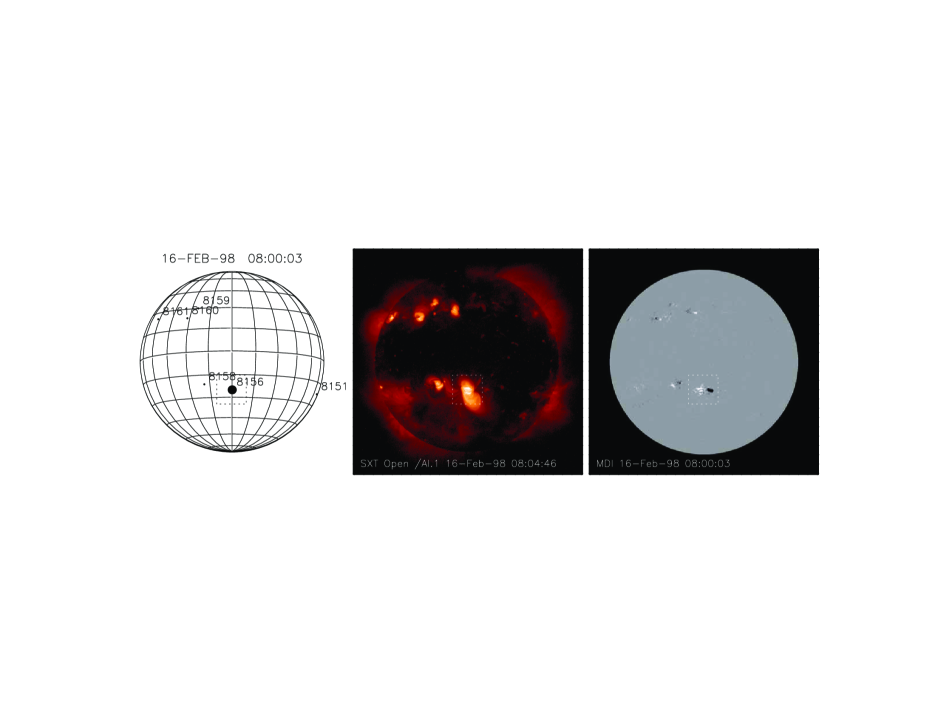
Figure 1: Observations of AR8156 on 1996 February 16 near 08:00 UT in SXT (center) and MDI (right). The field of view of the SXT partial frame images is indicated by the box.

From a visual inspection of the available data we selected observations of AR8156 taken 1998 February 16 near 8 UT. This region is shown in full-disk SXT and MDI images in Figure 1. The region of interest observed in SXT, EIT, and MDI is shown in Figure 2. These images represent the observations taken closest to the MDI magnetogram. The total intensities in the SXT partial frame images for this region during the period beginning 1998 February 15 23:30 UT and ending 1998 February 16 13:00 UT are generally within $\pm 20$% of the total intensities in these SXT images, indicating an absence of major flare activity during this time.

3 Static Modeling

To model the topology of this active region we use a simple potential field extrapolation of the photospheric magnetic field. For each MDI pixel with a field strength greater than 50 G we calculate a field line. Some representative field lines are shown in Figure 2. It is clear that such a simple model does not fully reproduce the observed topology of the images. The long loops in the bottom half of the images, for example, are shifted relative to the field lines computed from the potential field extrapolation. However, as we argued previously (Warren & Winebarger, 2006), our goal is not to reproduce the exact morphology of the active region. Rather, we are primarily interested in the more general properties of the active region emission, such as the total intensity or the distribution of intensities. The potential field extrapolation only serves to provide a realistic distribution of loop lengths.

One subtlety with coupling a potential field extrapolation with solutions to the hydrostatic loop equations is the difference in boundary conditions. The field lines originate in the photosphere where the plasma temperature is approximately 4,000 K. The boundary condition for the loop footpoints, however are typically set at 10,000 or 20,000 K in the numerical solutions to the hydrodynamic loop equations. Furthermore, studies of the topology of the quiet Sun have shown that a significant fraction of the field lines close at heights below 2.5 Mm, a typical chromospheric height (Close et al., 2003). To avoid these small scale loops we use the portion of the field line above 2.5 Mm in the modeling and exclude all field lines that do not reach this height.

For each of the 1956 field lines ultimately included in the simulation we calculate a solution to the hydrostatic loop equations using a numerical code written by Aad van Ballegooijen (e.g., Hussain et al. 2002; Schrijver & van Ballegooijen 2005). Following our previous work, our volumetric heating function is assumed to be

$$\epsilon_{S}=\epsilon_{0}\left(\frac{\bar{B}}{\bar{B}_{0}}\right)\left(\frac{L_{0}}{L}\right),$$ (1)

where $\bar{B}$ is the field strength averaged along the field line, and $L$ is the total loop length. We assume a constant cross section and a uniform distribution of heating along each loop. Note that the variation in gravity along the loop is determined from the geometry of the field line.

The numerical solution to the hydrostatic loop equation provides the variation in the density, temperature, and velocity along the loop. The temperatures, densities, and loop geometry are then used to compute the expected response in the SXT and EIT filters. For our work we use the CHIANTI atomic database (e.g. Dere et al., 1997) to compute the instrumental responses and the radiative losses used in the hydrostatic code (see Brooks & Warren 2006 for a discussion of the instrumental responses and radiative losses).

In our previous work the value for $\epsilon_{0}$ was chosen to be 0.0492 erg cm^-3 s^-1 so that a “typical” field line ($\bar{B}=\bar{B}_{0}$ and $L=L_{0}$) had an apex temperature of $T_{0}=4$ MK. We also found that for this value of $\epsilon_{0}$ a filling factor of about 10% was needed to reproduce the SXT emission observed in the Al.1 or AlMg filters. In the absence of information from the hotter SXT filters the value for $\epsilon_{0}$ is poorly constrained. The values adopted for the parameters $\bar{B}_{0}$ and $L_{0}$ are 76 G and 29 Mm respectively.

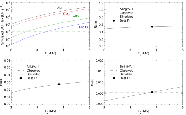
Figure 3: Simulated and observed SXT intensities for AR8156. (top left panel) The simulated intensities as a function of $T_{0}$ assuming a filling factor of unity. The observed intensities in each filter are indicated with the dotted lines. Simulations are calculated in steps of 0.5 MK. (other panels) Simulated filter ratios, which are independent of the filling factor, as a function of $T_{0}$. The observed filter ratios are indicated by the dotted lines. The best fit value for $T_{0}$ is also indicated on these plots.

For this active region we have observations in the hotter SXT filters so we have performed active region simulations for a range of $T_{0}$ (equivalently $\epsilon_{0}$) values. The resulting total intensities in each of the 4 filters as a function of $T_{0}$ are shown in Figure 3. It is clear from this figure that the static model cannot reproduce all of the SXT intensities for a filling factor of 1. For a filling factor of 1 the value of $T_{0}$ needed to reproduce the Al.1 intensity yields a Be119 intensity that is too low. Similarly, the value of $T_{0}$ that reproduces the Be119 intensity for a filling factor of 1 yields Al.1 intensities that are too large.

By doing a least squares fit of the simulation results to the observations and varying both the value of $T_{0}$ and the filling factor we find that we can reproduce all of the SXT intensities to within 10% for $T_{0}=3.8$ MK and a filling factor of 7.6%, values close to what we used in our previous work. These simulation results also highlight the importance of the SXT Al12 and Be119 filters in modeling the observations. The ratio between the Al.1 and AlMg filters is simply too shallow to be of any use in constraining the magnitude of the heating. The Al.1 to Be119 ratio, in contrast, varies by almost an order of magnitude as $T_{0}$ is varied from 2 to 5 MK.

The total intensity represents the minimum level of agreement between the simulation and the observations. The distribution of the simulated intensities must also look similar to what is observed. To transform the 1D intensities into 3D intensities we assume that the intensity at any point in space is related to the intensity on the field line by

$$I(x,y,z)=kI(x_{0},y_{0},z_{0})\exp\left[-\frac{\Delta^{2}}{2\sigma_{r}^{2}}\right]$$ (2)

where $\Delta^{2}=(x-x_{0})^{2}+(y-y_{0})^{2}+(z-z_{0})^{2}$ and $2.355\sigma_{r}$, the FWHM, is set equal to the assumed diameter of the flux tube. A normalization constant ($k$) is introduced so that the integrated intensity of over all space is equal to the intensity integrated along the field line. This approach for the visualization is based on the method used in Karpen et al. (2001).

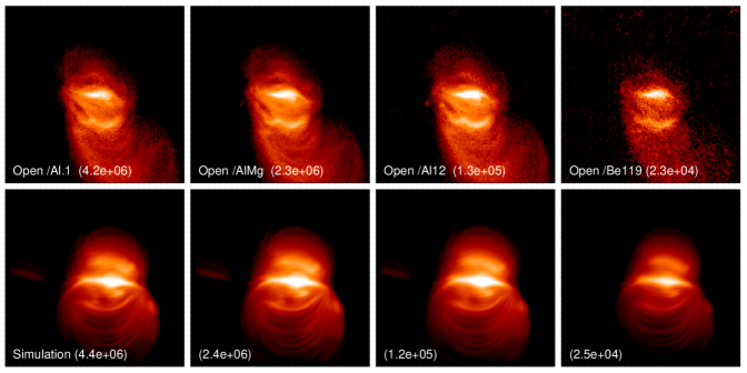
Figure 4: Observed and simulated SXT emission for AR8156. (top panels) Observed and simulated images. The calculated SXT images have been convolved with the SXT point spread function. The numbers in parentheses indicate the total intensity in the image. (bottom panels) The intensity distributions for the observed and simulated images.

The resulting simulated SXT images are shown in Figure 4 where they are compared with the observations. The simulations clearly do a reasonable job reproducing these data, particularly in the core of the active region. At the periphery of the active region the simulation does not match either the morphology of the emission or its absolute magnitude exactly. The general impression, however, is that the model intensities are generally similar to the observed intensities outside of the active region core even if the morphology doesn’t match exactly.

One change that we have made from our previous methodology (Warren & Winebarger, 2006) is to include all of the field lines with footpoint field strengths above 500 G. These field lines have been largely excluded in previous work because sunspots are generally faint in soft X-rays images (see Golub & Pasachoff 1997; Schrijver et al. 2004; Fludra & Ireland 2003). In these observations, however, the exclusion of the field lines rooted in strong field leads to small, but noticeable differences between the simulated and observed emission. As can be inferred from Figure 2, excluding these field lines leads to an absence of emission on either side of the bright feature in the center of the active region. This suggests that the algorithm used to select which field lines are included in the simulation needs to be studied more carefully.

The histograms of the intensities offer an additional point of comparison between the simulations and the observations. As shown in Figure 4, the distributions of the intensities are very similar in both cases, supporting the qualitative agreement between the visualizations and the actual solar images.

4 Dynamic Modeling

The principal difficulties with full hydrodynamic modeling of solar active regions are the many degrees of freedom available to parameterize the heating function and the computational difficulty of calculating the numerical solutions. For this exploratory study we make several simplifying assumptions. First, we consider dynamic simulations that are closely related to the static solutions. Since the static modeling of the SXT observations presented in the previous section adequately reproduces the total intensities, the distribution of intensities, and the general morphology of the images, it seems reasonable to consider dynamical heating that would reproduce the static solutions in some limit. Second, we utilize the time-averaged properties of these solutions in computing the simulated intensities. Our assumption is that the emission from a single field line in the static model actually results from the superposition of even finer, dynamical structures that are in various stages of heating and cooling. This is similar to the nanoflare picture of coronal heating (e.g., Parker, 1983; Cargill, 1994). Finally, we will also make use of grids of solutions where we interpolate to determine the simulated intensities rather than computing solutions for each field line individually.

In the static case we have used the average magnetic field strength and loop length to infer the volumetric heating rate ($\epsilon_{s}$) for each field line. For the dynamic case we consider volumetric heating rates of the form

$$\epsilon_{D}(t)=g(t)R\epsilon_{S}+\epsilon_{B},$$ (3)

where $g(t)$ is a step or boxcar function envelope on the heating, $\epsilon_{S}$ is the static heating rate determined from Equation 1, $R$ is a arbitrary scaling factor, and $\epsilon_{B}$ is a weak background heating rate that establishes a cool, tenuous equilibrium atmosphere in the loop. To solve the hydrodynamic loop equations numerically we use the NRL Solar Flux Tube Model (SOLFTM) code (e.g., Mariska, 1987; Mariska et al., 1989).

In the limit of an infinite heating window and $R=1$ the dynamic solutions would converge to the static solutions and all of the properties of the static simulation would be recovered. This is the primary motivation for our choice of the heating function given in Equation 3. The good agreement between the observations and the static model suggest that the energetics of the static model are not far off.

For $R=1$ and a finite duration to the heating we expect that the calculated SXT emission will generally be less than in the static case because it takes a finite time for chromospheric plasma to evaporate up into the loop. Thus simply truncating the heating will not produce acceptable results. If we increase the heating somewhat from the static case ($R>1$) and consider a finite duration we expect larger SXT intensities relative to the $R=1$, finite duration case since the evaporation will be faster and the temperatures will be higher with the increased heating. Since the time to fill the loop with plasma will depend on the sound crossing time ($\tau_{s}\sim L/c_{s}$, with $c_{s}$ the sound speed) the behavior of the dynamic solutions relative to the static solutions will also depend on loop length. For a finite duration to the heating the intensities in the dynamical simulations of the shorter loops will more closely resemble the results from the static solution.

An illustrative dynamical simulation is shown in Figure 5. Here $R=1.5$ and the heating duration is 200 s. For these parameters the apex densities are somewhat somewhat lower than the corresponding static solution. The time-averaging also reduces the SXT intensities significantly relative to their peak values. When the filling factor is included in the calculation of the SXT intensities from the static solutions, however, we see that the SXT intensities calculated from the two different simulations are very similar in all of the filters of interest.

Note that the computed intensities are somewhat dependent on the interval chosen for the time averaging. We assume that each small scale thread is heated once then allowed to cool fully before being heated again. In practice, we terminate the dynamical simulation when the apex temperature falls below 0.7 MK. The SOLFTM only has an adaptive mesh in the transition region and cannot resolve the formation of very cool material in the corona. Radiative losses become very large at low temperatures so the loops evolve very rapidly past this point and the time-averaged intensities should be only weakly dependent on when the dynamical simulation is stopped.

While calculations such as this, which show that the SXT intensities computed from the dynamical simulation and those computed from the static simulation can be comparable, are encouraging, they represent a special case. In general, for a fixed value of $R$ the ratio of the dynamic and static intensities will be greater than 1 for shorter loops and smaller than 1 for longer loops. We would like to know what would happen if we performed dynamical simulations for all of the loops in AR8156. Would the total intensities in the dynamical simulation match the observations?

The dynamical solutions we have investigated in this paper typically take about 500 s to perform on an Intel Pentium 4-based workstation. For our 1956 field lines this amounts to about 11 days of cpu time. While such calculations can be done in principle, particularly on massively parallel machines with 100s of nodes, they’re too lengthy for the exploratory work we consider here. To circumvent this computational limitation we consider a grid of solutions that encompass the range of loop lengths and heating rates that are present in our static simulation of this active region.

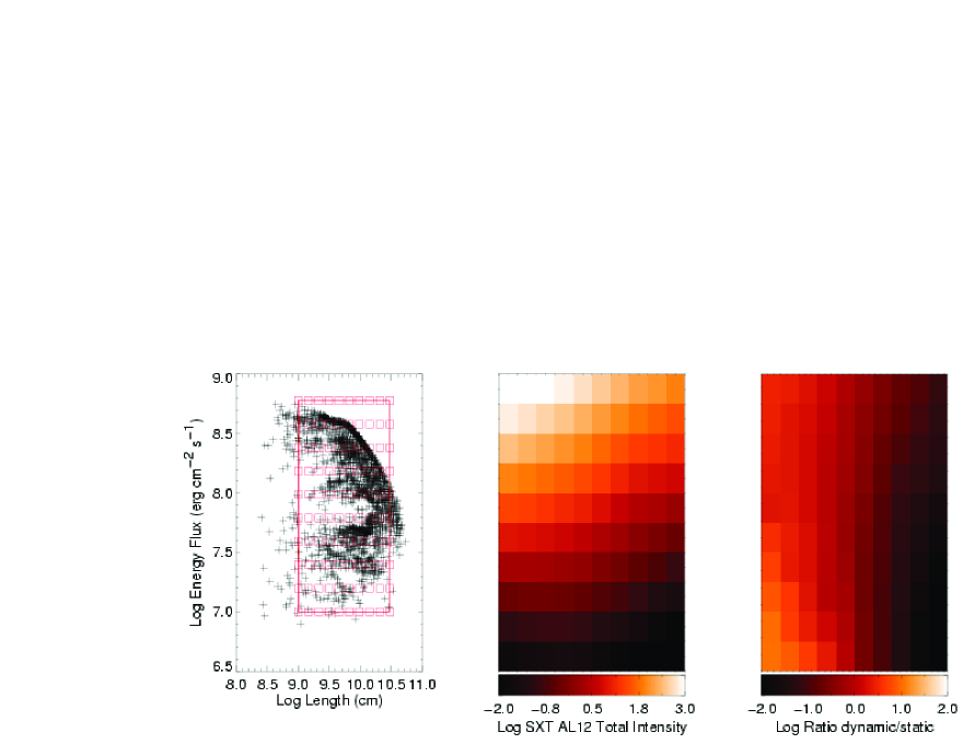
Figure 6: (left panel) A scatter plot of loop length ($L$) and energy flux ($\epsilon_{S}L$) for each field line in the static active region simulation. The red boxes indicate the values for which dynamic solutions have been calculated. The domain of the grid encompasses about 95% of the total SXT intensity in the active region. (middle panel) The total SXT Al12 intensity for each $L,\epsilon_{S}L$ pair in the grid for $R=1.5$. (right panel) The ratio of the total SXT Al12 intensities in the dynamic and static simulations for $R=1.5$. The other SXT filters yield total intensities and ratios very similar to what is shown here for Al12.

In Figure 6 we also show a plot of total loop length ($L$) and energy flux ($\epsilon_{S}L$) for each field line in the static simulation of AR8156. Note that we use the energy flux instead of the volumetric heating rate because, as indicated in the plot, these variables are largely uncorrelated and we can use a simple rectangular grid. The volumetric heating rate and the loop length, in contrast, are correlated. The procedure we adopt is to calculate dynamical solutions for the $L,\epsilon_{S}L$ pairs on this grid, determine the total SXT intensities for these solutions, and then use interpolation to estimate the SXT intensities for each field line in the simulation. To investigate the effects of varying $R$ on the dynamical solutions we have computed $10\times 10$ grids for $R=$1.0, 1.25, 1.5, 1.75, and 2.0 for a total of 500 dynamical simulations.

One important difference between these grid solutions and the static solutions discussed in the previous section is the loop geometry. In the static simulation the loop geometry is determined by the field line. In the dynamic simulation the loop is assumed to be perpendicular to the solar surface. Since the density scale height for high temperature loops is large this difference has only a small effect on the simulation of the SXT emission. The effect is much more pronounced for the lower temperature loops imaged in EIT and precludes the use of the interpolation grid for these intensities.

In Figure 6 we show the resulting SXT Al12 intensities for the $R=1.5$ grid of solutions. The most intense loops in the dynamic simulations are the shortest loops with the most intense heating. These loops come the closest to reaching equilibrium parameters with the finite duration heating. The faintest loops are the longest loops with the weakest heating. In Figure 6 we also show the ratio of the SXT intensities from the dynamic and static simulations. That is, we compare the total intensity determined from the static solution with a heating rate of $\epsilon_{S}$ with the total intensity determined with the time dependent heating rate $\epsilon_{D}$ given in Equation 3. These ratios indicate that for a significant region of this parameter space the total intensities in the dynamic heating are close to those computed for the static simulations. The shorter field lines are somewhat more intense while the longer field lines are generally fainter. This suggests that the dynamic intensities integrated over all of the field lines should produce results similar to the static simulation. As expected, for smaller values of $R$ these ratios are systematically smaller and for larger values of $R$ these ratios are systematically larger.

We have used the results from all of the dynamic simulation grids to estimate the total SXT intensity in each filter as a function of $R$. The results are shown in Figure 7. For $R=1$ the total intensities are smaller than what is observed by about 50%. For $R=2$ the intensities are all too large by about 100%. For the $R=1.5$ case, which we have highlighted in Figures 5 and 6, the simulated total intensities are within 20% of the measurements in all 4 filters, and this case come closest to reproducing the observations. The differences between the model calculations and the observations are not systematic. The calculated Al12 and Be119 intensities are very close to the observations while the Al1 and AlMg are a little too high. The duration of the heating, which we have chosen to be 200 s, may explain this discrepancy, at least partially. If the heating were reduced in duration stronger heating (larger $R$) would be required to match the observed intensities. This would lead to higher temperatures and lead to somewhat different ratios among three filters.

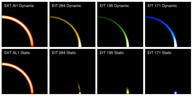
Figure 8: The distribution of emission from dynamical and static heating models of the field line shown in Figure 5. The same logarithmic scaling is used for each pair of images. The width of the point spread function has been chosen arbitrarily. The intensities shown for the dynamic case are time-averaged. The morphology of the loop imaged in SXT is very similar in both the dynamic and static heating scenarios. The dynamic heating gives rise to a much more even distribution of intensity along the field line at the cooler temperatures.

One of the primary motivations for introducing dynamic modeling is the inability of static models to account for the EUV observations at lower temperatures. Because we have used interpolation grids to infer the intensities it is not possible to compute images similar to those presented in Figure 4. We can, however, consider the morphology of individual loops with the static and dynamic heating scenarios. To investigate this we calculate the time-averaged intensity in SXT and EIT along the loop. As illustrated in Figure 8, the dynamic heating is clearly moving in the right direction. The morphology of the high temperature plasma imaged with SXT is largely unchanged in the dynamic simulation while the EUV emission shows full loops. This suggests that the dynamic simulations of active regions will look much closer to the observations shown in Figure 2 than the synthetic images calculated from static heating models.

One implication of Figure 8 is that relatively cool loops imaged in the EUV should be co-spatial with high temperature loops imaged in soft X-rays. There is some evidence that this is not observed. Schmieder et al. (2004) and Nitta (2000), for example, argue that the EUV loops may be observed near soft X-ray loops, but that they are generally not co-spatial. It is possible, however, that the geometry of the loops changes as they cool (Winebarger & Warren, 2005). Antiochos et al. (2003) suggest that the observed EUV loop emission in an active region is not bright enough to account for the cooling of soft X-ray loops. However, the contrast between the background corona and the EUV loops is low (Cirtain et al., 2006), and it is possible that the total EUV intensity in an active region is consistent with the cooling of high temperature loops.

5 Summary and Discussion

We have investigated the use of static and dynamic heating models in the simulation of AR8156. Recent work has shown that static models can capture many of the observed properties of the high temperature soft X-ray emission from solar active regions and our results confirm this. We are able to reproduce both the total intensity and the general morphology of this active region with a static heating model. Furthermore, our results show that this agreement extends to the the hotter SXT filters which have not been considered before.

The application of dynamic heating models to active region emission on this scale has not been considered previously. Only the properties of individual loops have been explored (e.g. Warren et al., 2002). The computational complexity of the dynamical simulations precludes the calculation of individual solutions for each field line and we have utilized interpolation grids for estimating the expected SXT intensities for each field line. We find that it is possible to reproduce the observed SXT intensities in 4 filters, including the high temperature Al12 and Be119 filters, using the dynamical model.

Conceptually, the simple dynamical heating model investigated here, where we assume that the emission from a solar feature results from the superposition of many, very fine structures that are in various stages of heating and cooling, is closely related to the nanoflare model of coronal heating (e.g., Parker, 1983; Cargill, 1994). The use of time-averaged intensities computed from the dynamical simulations implicitly assumes that the heating is very coherent, with each infinitesimal thread being heated once and then allowed to cool and drain before being heated again. Other scenarios are possible, such as heating events on larger scale threads that are distributed randomly in time. The spatial and temporal characteristics of coronal heating is likely to fall somewhere in between these extremes. The analysis of high spatial resolution (0.5″) EUV images suggests that current solar instrumentation may be close to resolving individual threads in the corona (Aschwanden, 2005; Aschwanden & Nightingale, 2005), but considerable work remains to be done to determine the fundamental spatial scale for coronal heating.

The geometrical properties of coronal threads is also unclear at present. We have assumed constant cross sections in our modeling, consistent with the observational results (Klimchuk et al., 1992; Watko & Klimchuk, 2000). In the static modeling of solar active regions there has been some evidence that the loops with expanding cross sections better reproduce the observations (Schrijver et al., 2004; Warren & Winebarger, 2006). Detailed comparisons between simulated and observed solar images are needed to resolve this issue.

Despite the many limitations to our modeling the results that we have presented are encouraging and provide a framework for further exploration. The highest priority for future work is the full dynamical simulation of solar active regions without the use of interpolation grids so that synthetic soft X-ray and EUV images can be computed and compared with observations. Another priority is the comparison of active region simulations with spatially and spectrally resolved observations from the upcoming Solar-B mission. Spectral diagnostics, such as Doppler velocities and nonthermal widths, are another dimension that have not been explored in the context of this modeling.

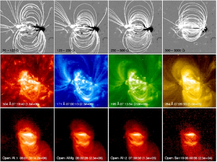
Figure 2: (top panels) Selected field lines from the potential field extrapolation of the MDI magnetogram taken at 08:00:03 UT. (middle panels) EIT synoptic images of AR8156 in all four EIT wavelengths. (bottom panels) SXT images in four filters.

Figure 5: A comparison of static and dynamic simulations of SXT emission. The parameters for the static case are $L=37$ Mm and $\epsilon_{S}=0.0126$ erg cm^-3 s^-1, and are typical of the active region simulation. For the dynamic case $R=1.5$ and the heating duration is 200 s. (right panels) The evolution of the temperatures and densities averaged over the top 10% of the loop apex. (right panels) The evolution of the intensities in 4 SXT filters. The SXT intensities from the static model, including the filling factor from the active region simulation, are also shown. For this case the SXT intensities from the time-averaged dynamic simulation are very close to those from the static simulation.

Figure 7: Total SXT intensities from the dynamical simulations as a function of $R$, the ratio of impulsive to static heating rate. The dotted lines indicate the observed intensities. The simulation grid with $R=1.5$ best approximates the observed intensities.

References

- Antiochos et al. (2003) Antiochos, S. K., Karpen, J. T., DeLuca, E. E., Golub, L., & Hamilton, P. 2003, ApJ, 590, 547
- Aschwanden (2005) Aschwanden, M. J. 2005, ApJ, 634, L193
- Aschwanden & Nightingale (2005) Aschwanden, M. J., & Nightingale, R. W. 2005, ApJ, 633, 499
- Aschwanden et al. (2001) Aschwanden, M. J., Schrijver, C. J., & Alexander, D. 2001, ApJ, 550, 1036
- Brooks & Warren (2006) Brooks, D. H., & Warren, H. P. 2006, ApJS, 164, 202
- Cargill (1994) Cargill, P. J. 1994, ApJ, 422, 381
- Cirtain et al. (2006) Cirtain, J., Martens, P. C. H., Acton, L. W., & Weber, M. 2006, Sol. Phys., 235, 295
- Close et al. (2003) Close, R. M., Parnell, C. E., Mackay, D. H., & Priest, E. R. 2003, Sol. Phys., 212, 251
- Delaboudinière et al. (1995) Delaboudinière, J.-P., et al. 1995, Sol. Phys., 162, 291
- Dere et al. (1997) Dere, K. P., Landi, E., Mason, H. E., Monsignori Fossi, B. C., & Young, P. R. 1997, A&AS, 125, 149
- Fludra & Ireland (2003) Fludra, A., & Ireland, J. 2003, in The Future of Cool-Star Astrophysics: 12th Cambridge Workshop on Cool Stars , Stellar Systems, and the Sun (2001 July 30 - August 3), eds. A. Brown, G.M. Harper, and T.R. Ayres, (University of Colorado), 2003, p. 220-229., 220
- Golub & Pasachoff (1997) Golub, L., & Pasachoff, J. M. 1997, The Solar Corona (The Solar Corona, by Leon Golub and Jay M. Pasachoff, ISBN 0521480825. Cambridge, UK: Cambridge University Press, September 1997.)
- Hussain et al. (2002) Hussain, G. A. J., van Ballegooijen, A. A., Jardine, M., & Collier Cameron, A. 2002, ApJ, 575, 1078
- Karpen et al. (2001) Karpen, J. T., Antiochos, S. K., Hohensee, M., Klimchuk, J. A., & MacNeice, P. J. 2001, ApJ, 553, L85
- Klimchuk (2006) Klimchuk, J. A. 2006, Sol. Phys., 234, 41
- Klimchuk et al. (1992) Klimchuk, J. A., Lemen, J. R., Feldman, U., Tsuneta, S., & Uchida, Y. 1992, PASJ, 44, L181
- Mariska (1987) Mariska, J. T. 1987, ApJ, 319, 465
- Mariska et al. (1989) Mariska, J. T., Emslie, A. G., & Li, P. 1989, ApJ, 341, 1067
- Nitta (2000) Nitta, N. 2000, Sol. Phys., 195, 123
- Parker (1983) Parker, E. N. 1983, ApJ, 264, 642
- Patsourakos & Klimchuk (2006) Patsourakos, S., & Klimchuk, J. A. 2006, ApJ, 647, 1452
- Reale & Peres (2000) Reale, F., & Peres, G. 2000, ApJ, 528, L45
- Scherrer et al. (1995) Scherrer, P. H., et al. 1995, Sol. Phys., 162, 129
- Schmieder et al. (2004) Schmieder, B., Rust, D. M., Georgoulis, M. K., Démoulin, P., & Bernasconi, P. N. 2004, ApJ, 601, 530
- Schrijver et al. (2004) Schrijver, C. J., Sandman, A. W., Aschwanden, M. J., & DeRosa, M. L. 2004, ApJ, 615, 512
- Schrijver & Title (2005) Schrijver, C. J., & Title, A. M. 2005, ApJ, 619, 1077
- Schrijver & van Ballegooijen (2005) Schrijver, C. J., & van Ballegooijen, A. A. 2005, ApJ, 630, 552
- Spadaro et al. (2003) Spadaro, D., Lanza, A. F., Lanzafame, A. C., Karpen, J. T., Antiochos, S. K., Klimchuk, J. A., & MacNeice, P. J. 2003, ApJ, 582, 486
- Testa et al. (2005) Testa, P., Peres, G., & Reale, F. 2005, ApJ, 622, 695
- Tsuneta et al. (1991) Tsuneta, S., et al. 1991, Solar Phys., 136, 37
- Ugarte-Urra et al. (2006) Ugarte-Urra, I., Winebarger, A. R., & Warren, H. P. 2006, ApJ, 643, 1245