Galaxy clusters at $\bf 0.6<z<1.4$ in the UKIDSS Ultra Deep Survey Early Data Release

Abstract

We present the first cluster catalogue extracted from the UKIRT Infrared Deep Sky Survey Early Data Release. The catalogue is created using UKIDSS Ultra Deep Survey infrared $J$ and $K$ data combined with 3.6 $\mu$m and 4.5 $\mu$m Spitzer bands and optical $BVRi^{\prime}z^{\prime}$ imaging from the Subaru Telescope over 0.5 square degrees in the Subaru XMM-Newton Deep Field. We have created a new cluster-detection algorithm, based on the Friends-Of-Friends and Voronoi Tessellation methods, which utilises probability distribution functions derived from a photometric redshift analysis. We employ mock catalogues to understand the selection effects and contamination associated with the algorithm. The cluster catalogue contains 13 clusters at redshifts 0.61 $\leq z\leq$ 1.39 with luminosities $10{\rm L^{*}}\mathrel{\hbox{\hbox to0.0pt{\hbox{\lower 2.0pt\hbox{$\sim$}}\hss}\raise 2.0pt\hbox{$<$}}}L_{\rm tot}\mathrel{\hbox{\hbox to0.0pt{\hbox{\lower 2.0pt\hbox{$\sim$}}\hss}\raise 2.0pt\hbox{$<$}}}50\rm L^{*}$, corresponding to masses $5\times 10^{13}~{}{\rm M_{\odot}}\mathrel{\hbox{\hbox to0.0pt{\hbox{\lower 2.0pt\hbox{$\sim$}}\hss}\raise 2.0pt\hbox{$<$}}}M_{cluster}\mathrel{\hbox{\hbox to0.0pt{\hbox{\lower 2.0pt\hbox{$\sim$}}\hss}\raise 2.0pt\hbox{$<$}}}3\times 10^{14}~{}\rm M_{\odot}$ for $\frac{M/\rm M_{\odot}}{L/\rm L_{\odot}}=75h$. The measured sky surface density of $\sim 10~{}\rm deg^{-2}$ for high-redshift ($z=0.5-1.5$), massive ($>10^{14}~{}\rm M_{\odot}$) clusters is precisely in line with theoretical predictions presented by Kneissl et al. (2001).

1 Introduction

Distant galaxy clusters are used in a wide range of cosmological and astrophysical contexts. For instance, cluster studies illuminate how dark matter haloes collapse and large-scale structure forms and evolves. Comparisons of the evolution of the cluster mass-function to that predicted by $N$-body simulations (Evrard et al. 2002) or the Press-Schechter formalism (Press & Schechter 1974) and its variants place strong constraints on cosmological parameters such as the mass density ($\Omega_{\rm M}$) and the amplitude of the mass fluctuations in the early Universe ($\sigma_{8}$) (e.g. Eke et al. 1998). Further, high-redshift clusters can help constrain feedback processes caused by star-formation and Active Galactic Nuclei (e.g. Silk & Rees 1998). Unfortunately few $z>1$ clusters have been identified, and the vast majority of these are from X-ray surveys (e.g. using XMM-Newton; Stanford et al. 2006).

X-ray selected cluster surveys (e.g. Mullis et al. 2005) have succeeded in finding clusters with luminous intra-cluster media. Some follow-up observations exploiting the Sunyaev-Zel’dovich (SZ) effect have been successful (e.g. Jones et al. 2005) and comprehensive SZ surveys are underway (Kneissl et al. 2001). Optical selection of clusters is complementary to these studies (Gilbank et al. 2004) as it is based on other cluster properties, e.g. optical vs. X-ray luminosity or the SZ decrement of the cluster gas. An added advantage of using optical data is the possibility of employing a photometric redshift analysis to derive the distance to the clusters and gain a three-dimensional perspective. Optical cluster searches however have been stymied at high redshifts by the fact that the 4000Å break (ubiquitous for the early-type, red galaxies dominant in clusters) shifts out of the $I$-band into the near-infrared. Recent developments have seen the advent of large near-infrared cameras like the Wide Field Infrared Camera (WFCAM) on the United Kingdom Infrared Telescope (UKIRT). WFCAM is now undertaking the UKIRT Infrared Deep Sky Survey (UKIDSS, Lawrence et al. 2006).

In this letter we use the UKIDSS Ultra Deep Survey (UDS) Early Data Release (EDR, Dye et al. 2006) to find clusters in the redshift range $0.5\leq z\leq 1.5$. The clusters are found by applying adaptations of two cluster selection methods: the Voronoi Tessellation technique (Ebeling & Wiedenmann 1993) and the Friends-Of-Friends method (Huchra & Geller 1982). We describe the data and the determination of photometric redshifts in §2, and the cluster-detection algorithm and simulations using mock catalogues in §3. The cluster catalogue is presented in §4 and in §5 we summarize our conclusions. Throughout this letter we assume $H_{\circ}=71~{}{\rm km~{}s^{-1}Mpc^{-1}}$, $\Omega_{\rm M}=0.27$, and $\Omega_{\Lambda}=0.73$. All magnitudes quoted are in the AB-system.

2 Data and Photometric Redshifts

We use three sources of data: near-infrared $J$ and $K$ data from the UDS EDR (Foucaud et al. 2006); 3.6$\mu$m and 4.5$\mu$m bands from the Spitzer Wide-area InfraRed Extragalactic survey (SWIRE, Lonsdale et al. 2005); and optical $BVRi^{\prime}z^{\prime}$ Subaru data over the Subaru XMM-Newton Deep Field (SXDF, Furusawa et al. in prep.). The area of our cluster survey is 0.5 sq. deg. with 34.2${}^{\circ}<$ RA $<34.8^{\circ}$ and $-$5.4${}^{\circ}<$ Dec. $<-4.6.^{\circ}$ (02:16:48.00 $<$ RA $<$ 02:19:13.20, $-$05:25:12.0 $<$ Dec $<$ $-$04:38:17.1). The galaxy catalogue includes the objects with a detection in $i^{\prime}$, $J$ and $K$ and to exclude stars we impose a criterion of SExtractor stellarity index $<$ 0.8 in $i^{\prime}$ and $K$ (e.g. Bertin & Arnouts 1996). The depth of the catalogue is limited by the UDS EDR 5$\sigma$ magnitude limits of $K_{\rm AB,lim}=J_{\rm AB,lim}=22.5$. We derive photometric redshifts by fitting a spectral energy distribution (SED) template to each object’s photometry using the Hyperz code (Bolzonella et al 2000). The galaxy templates are generated with the stellar population synthesis code GALAXEV (Bruzual & Charlot 2003) and cover a range of different star formation rates with timescales $\tau$ from 0.1 to 30 Gyr. We adopt a flat prior for galaxy luminosity up to a maximum of $L=10\rm L^{*}$ (assuming a passively evolving elliptical galaxy) in the observed $K$-band and calculate the marginalised posterior redshift probability functions. Our photometric redshift catalogue comprises 19300 objects in the range $0.1\leq z\leq 2.0$.

2.1 Reliability of the photometric redshifts

To test the reliability of the photometric redshifts we run Hyperz with the same templates on spectroscopically identified objects in the SXDF (Yamada et al. 2005; Simpson et al. 2006). The spectroscopic and photometric redshifts are consistent, with a photometric redshift error of $\sigma_{z}=0.08$ over $0.5\leq z\leq 1.5$ and no obvious systematic offset. However, an examination of the number of galaxies in the photometric-redshift catalogue as a function of redshift, $N(z)$, reveals spikes in the redshift distribution. The shape of the distribution is constant across the field which indicates the spikes are not caused by large-scale structure but by aliasing effects inherent to photometric redshift methods employing many more templates than data points (e.g. Rowan-Robinson 2003). A serious concern is the detection of spurious clusters due to this focussing in redshift. We therefore create a second redshift catalogue using four empirically derived SEDs from Coleman, Wu & Weedman (1980), supplied with the Hyperz code. The new galaxy redshift probability functions are broader; the spikes disappear yielding a smoother $N(z)$ distribution. However, a comparison of the spectroscopic redshifts reveal that the redshift is systematically underestimated at $z\mathrel{\hbox{\hbox to0.0pt{\hbox{\lower 2.0pt\hbox{$\sim$}}\hss}\raise 2.0pt\hbox{$>$}}}0.5$, with an offset of $\Delta z=0.15$ at $z\sim 1$.

In summary, an examination of the accuracy of the photometric redshifts reveals a sensitivity to the templates used in the photometric redshift estimation. Redshifts quoted in this letter use the Bruzual & Charlot templates as the spectroscopic sample show these to be most accurate. However to avoid false cluster detections due to the spikiness in the $N(z)$ distribution we limit ourselves in this letter to the clusters that are isolated in both photometric redshift catalogues and are therefore considered to be robust detections.

3 The Algorithm

The cluster-detection algorithm is described in detail in van Breukelen et al. (in prep.). Here we present only a brief outline of the procedures we employ.

Two common problems of optically selected cluster samples are the detection of spurious clusters, and the chance projection of fore- and background galaxies into the real clusters. This is caused by selection biases inherent to any detection algorithm and the fact that photometric redshift probability functions (z-PDFs) can take any form, exhibiting errors that may be many times larger than the redshift range of the cluster. To reduce these difficulties we (i) use two substantially different cluster-detection methods to minimize the number of false detections, and (ii) utilize the full z-PDFs rather than the best redshift estimate with an associated error. For each method we sample the z-PDFs to create 500 Monte-Carlo (MC) realisations of the 3-D galaxy distribution. These are divided in slices of $\Delta z=0.05$ in which the cluster candidates are identified. Since the error on the photometric redshift is larger than the width of the redshift slices, each cluster-candidate is typically found in several adjoining slices. We determine the final cluster-redshift by taking the average of the redshifts at which the cluster occurs, weighted by the corresponding number of MC-realisations. We assign a ‘reliability factor’ $F$ to each of the clusters which is the total fraction of MC-realisations in which the cluster is detected. The algorithm uses the Voronoi Tessellation technique (VT), and the Friends-Of-Friends method (FOF) to detect cluster candidates in the redshift slices. One of the principal advantages of the VT method is that it is relatively unbiased as it does not look for a particular source geometry (e.g. Ramella et al. 2001). The field of galaxies is divided into Voronoi Cells, each containing one object: the nucleus. The reciprocal of the area of the VT cells translates to a local density. Overdense regions in the plane are found by fitting a function (see Kiang 1966) to the density distribution of all VT cells in the field; cluster candidates are the groups of cells of a significantly higher density than the mean background density. The Friends-Of-Friends (FOF) algorithm groups galaxies with a smaller separation than a projected linking distance $D_{\rm link}$ (‘friends’). When spectroscopic data is available, the ‘friends’ are also subject to a linking velocity $\Delta V\leq V_{\rm link}$ (e.g. Tucker et al., 2002). With photometric redshifts only galaxies within the same redshift slice are linked (see Botzler et al. 2004). If a group comprises a number of galaxies larger than $n_{\rm min}$ it is considered a cluster candidate.

We create mock catalogues that mimic the real data to quantify the various selection effects and expected contaminants. These simulations also lead to estimates of the total stellar luminosity of the clusters found in the real data.

3.1 Simulated Cluster Catalogues

We create catalogues with a galaxy distribution randomly placed in the field with $0.1\leq z\leq 2.0$. The galaxy luminosities and number densities are determined by the $K$-band luminosity function of Cole et al. (2001), with the simplifying assumption of passive evolution with formation redshift $z_{form}=10$. A detection limit of $K<22.5$ is imposed to match the 5-$\sigma$ limit of the UDS EDR data. The number of galaxies as a function of magnitude in each mock catalogue is entirely consistent with the number counts in the UDS catalogue to this limit. We superimpose simulated clusters of total mass $M=0.5,1.0,2.0,10,20\times 10^{14}~{}\rm M_{\odot}$, assuming $\frac{M/\rm M_{\odot}}{L/\rm L_{\odot}}=75h$ (Rines et al. 2001) and applying a cluster $K-$band luminosity function (Lin et al. 2004). The galaxies are spatially distributed within the cluster according to an NFW profile (Navarro, Frenk & White, 1997) with a cut-off radius of 1 Mpc. For the simulated clusters of mass $>1.0\times 10^{15}~{}\rm M_{\odot}$ this is smaller than the virial radius; however we do not find such high mass clusters in our data (see Section 4) and the effect of the cut-off is therefore negligible. The clusters are placed at redshifts $z=0.1,0.2,...,2.0$. Each combination of mass and redshift is represented in ten randomly created catalogues. We offset the redshift of all galaxies randomly with a factor equal to the errors in the real data. Each galaxy receives a z-PDF taken from the data by selecting an object with corresponding redshift.

The VT and FOF methods each have two free parameters. For FOF these are the linking distance in proper coordinates, $D_{\rm link}$, and the minimum number of galaxies in a cluster, $n_{\rm min}$. Guided by Botzler et al. (2004) we experiment with values between 0.125 Mpc $\leq D_{\rm link}\leq$ 0.175 Mpc, and $3\leq n_{\rm min}\leq 5$. For VT the parameters are the maximum probability of an overdensity being a background fluctuation, $p_{\rm bg}$, and the lower limit on the cell density, $f_{\rm min}$. We follow the method of Ebeling & Wiedenmann (1993) and set $p_{\rm bg}$ to 10%. For $f_{\rm min}$ we try values of $1.2-2.2$, where $f=1.0$ is the mean cell density of the field. We use the parameters that optimize the algorithm’s performance: $D_{\rm link}=0.175$ Mpc, $n_{\rm min}=5$, and $f_{\rm min}=1.74$. Since both methods use different measures to isolate clusters (galaxy density in VT versus separation in FOF) the false detections in both do not coincide. Therefore by cross-correlating the output of the two methods the spurious sources due to biases in the algorithms disappear, which reduces the contamination to chance galaxy groupings. There is no obvious bias due to cluster morphology (for a full treatment of biases and contanimation see van Breukelen et al in prep.).

We compare the recovered cluster galaxies to the input galaxies of the mock clusters. VT tends to include all galaxies in a large area around the cluster core (see for example the left-hand panel of Fig. 1). The number of recovered cluster members, $N_{\rm gal}$, in any cluster is sensitive to the local field density. By contrast, the galaxy members recovered by FOF are more centrally concentrated; the total number per cluster is consistent throughout the random realisations of the catalogues. Thus we use both methods to detect the clusters and only FOF to calculate $N_{\rm gal}$. This is done by taking all galaxies that occur in the cluster at $>15\%$ of the MC-realisations in which the cluster itself is detected. The galaxies that appear in a smaller fraction of MC-realisations are very likely to be interlopers from different redshifts. Calculating $N_{\rm gal}$ for all cluster-masses at all redshifts yields functions of $N_{\rm gal}$ vs. $z$ for constant mass or total luminosity. At $z>1.5$ only clusters of masses $M\geq 1.0\times 10^{15}~{}\rm M_{\odot}$ or $L>170\rm L^{*}$ can be detected with $\sim$ 50% completeness. At redshifts of $z<0.5$ our field of view is $\mathrel{\hbox{\hbox to0.0pt{\hbox{\lower 2.0pt\hbox{$\sim$}}\hss}\raise 2.0pt\hbox{$<$}}}$ 10 times the typical cluster size of 1 Mpc. Hence we limit our redshift range to $0.5\leq z\leq 1.5$, allowing the detection of clusters of luminosity $L\mathrel{\hbox{\hbox to0.0pt{\hbox{\lower 2.0pt\hbox{$\sim$}}\hss}\raise 2.0pt\hbox{$>$}}}10\rm L^{*}$ at $z\sim 0.5$ to $L\mathrel{\hbox{\hbox to0.0pt{\hbox{\lower 2.0pt\hbox{$\sim$}}\hss}\raise 2.0pt\hbox{$>$}}}170\rm L^{*}$ at $z\sim 1.5$.

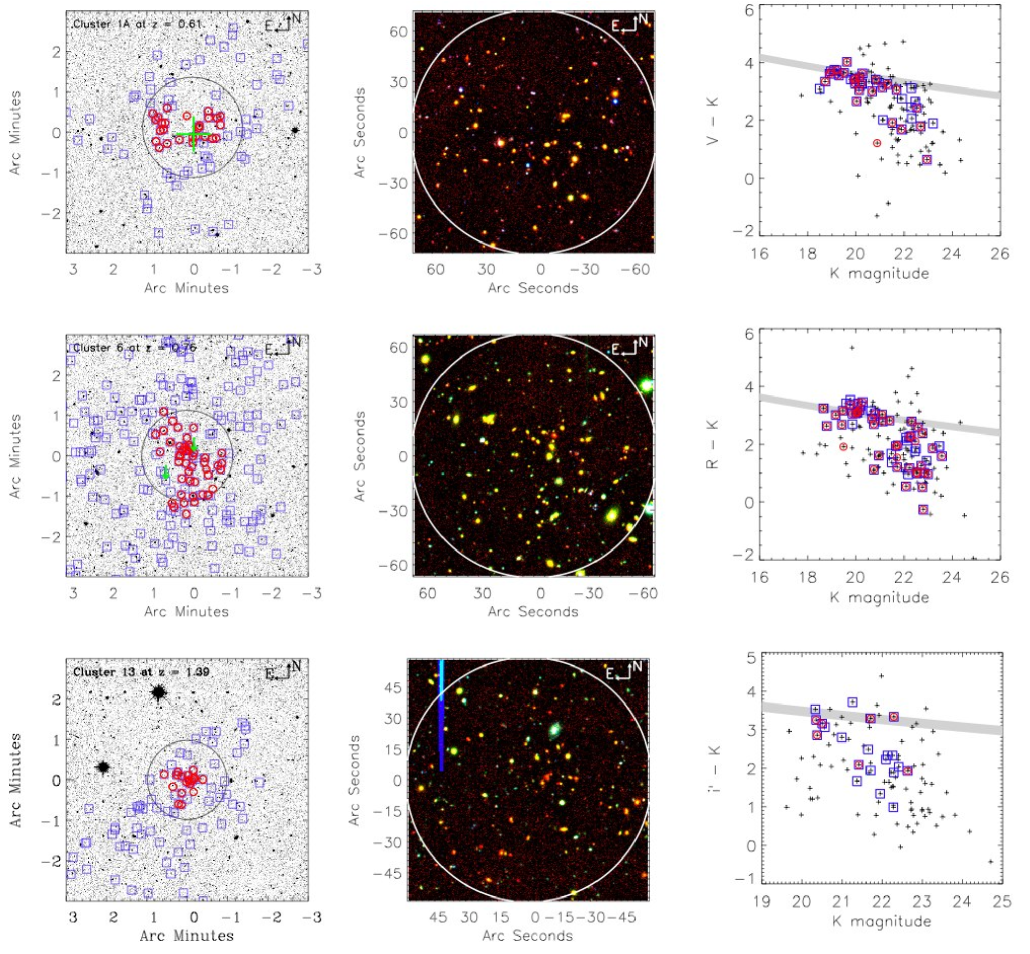
Figure 1: Clusters 1, 6, and 13 spanning the redshift range of our detections. Left: $K$-band images; the large circle shows a 1 Mpc region around the cluster; the blue squares and red circles are cluster members as given by VT and FOF respectively. ID 1: the green cross denotes an extended X-ray source. ID 6: the green arrows point out galaxies with $z_{\rm spec}=0.87$. Middle: $Bz^{\prime}K$ images of the central 1 Mpc region. Right: colour-magnitude plots of the clusters: the colour is the reddest filter shortward of 4000Å (restframe) minus $K$. The crosses are all galaxies within the central 1 Mpc region, otherwise the symbols are the same as in the left-hand panel. The grey band is the modelled red sequence.

4 Results: The Cluster Catalogue

ID	RA	Dec.	$z_{\rm phot}$	$N_{\rm gal}$	$L_{\rm tot}$	Mass	$F_{\rm fof}$	$F_{\rm vt}$	$z_{\rm spec}$
	[h m s]	[∘ ′ ′′]			[$\rm L^{*}$]	[10${}^{14}~{}\rm M_{\odot}$]
1A*	02 17 35.3	-05 13 16	0.61 $\pm$ 0.05	24	19	1.1	0.8	0.5	0.65†
1B	02 17 31.5	-05 10 59	0.65 $\pm$ 0.07	10	10	0.5	0.4	0.4	-
2A	02 16 59.9	-05 10 39	0.64 $\pm$ 0.02	11	10	0.6	0.7	0.2	-
2B	02 16 51.7	-05 12 15	0.71 $\pm$ 0.05	17	17	1.0	0.7	0.5	-
3	02 18 34.9	-04 58 05	0.66 $\pm$ 0.07	23	19	1.1	1.0	0.7	-
4	02 18 09.0	-05 21 54	0.67 $\pm$ 0.03	19	17	1.0	0.5	0.3	-
5	02 18 00.4	-04 42 58	0.71 $\pm$ 0.03	8	10	0.5	0.3	0.2	-
6*	02 18 32.7	-05 01 04	0.76 $\pm$ 0.12	36	46	2.7	1.0	0.8	0.87‡
7	02 19 03.5	-04 42 33	0.78 $\pm$ 0.06	17	18	1.0	0.7	0.3	-
8	02 17 56.4	-05 02 46	0.79 $\pm$ 0.07	11	11	0.6	0.2	0.2	-
9	02 17 21.4	-05 11 30	0.80 $\pm$ 0.06	15	17	1.0	0.2	0.6	0.93††
10	02 18 03.2	-05 00 01	0.94 $\pm$ 0.14	17	36	2.1	0.4	0.8	-‡‡
11A	02 18 06.4	-05 03 25	0.95 $\pm$ 0.11	24	48	2.8	0.6	0.8	1.06‡
11B	02 18 15.5	-05 02 50	0.98 $\pm$ 0.09	12	18	1.0	0.3	0.4	0.92‡
12	02 17 07.4	-04 46 44	1.01 $\pm$ 0.06	16	39	2.3	0.3	0.6	1.102†††
13*	02 18 10.5	-05 01 05	1.39 $\pm$ 0.07	7	41	2.4	0.2	0.6	-
14	02 18 37.3	-04 48 50	0.77 $\pm$ 0.07	11	11	0.6	0.4	0.3	-

Table 1: The cluster catalogue ordered by redshift. The position (J2000) is the centroid of the cluster galaxies. $N_{\rm gal}$ is the number of cluster galaxies detected by FOF with $K<22.5;$ $L_{\rm tot}$ is the estimated total luminosity of the cluster and mass the inferred total cluster mass; $F_{\rm fof}$ and $F_{\rm vt}$ are the reliability factors given respectively by FOF and VT. The possible spectroscopic redshift is given as $z_{\rm spec}$; clusters marked with a star [*] are shown in Fig. 1. All clusters above the line are robust; ID 14 was not recovered with the alternative photometric redshift catalogue. †  Extended X-ray-detected cluster (Kolokotronis et al. 2006); $z_{\rm spec}$ from Geach et al. (in prep). ‡  Two galaxies in each of the clusters are found at this redshift (Yamada et al. 2005). ††  Four galaxies in the cluster are found at this redshift (Yamada et al. 2005). ‡‡  Potential cluster galaxies have $z_{\rm spec}=$0.874, 0.96, and 1.095; super-position effects may be exaggerating the richness of this cluster. †††  Redshift of a QSO possibly associated with the cluster (Sharp et al. 2002).

Our final cluster catalogue comprises all clusters found by both VT and FOF with a reliability factor of $F>0.2$ to exclude false detections. We calculate the redshift by averaging the cluster redshift given by the VT and FOF methods. This results in 14 clusters at $0.61\leq z\leq 1.39$; Table 1 lists all the clusters with their positions and properties (full details of the cluster galaxies are available on request). The redshift error given in Table 1 combines the errors given by VT and FOF and reflects the range of redshift slices in which the cluster is detected. Although the cluster-finding method is sensitive to clusters down to a luminosity of $\sim 10\rm L^{*}$ we are limited by the relatively large systematic errors from the photometric redshifts. The 13 clusters ‘above the line’ in Table 1 were also detected in our alternative photometric redshift catalogue (see Section 2.1), although sometimes only at the $F_{\rm fof}$ and $F_{\rm vt}>0.1$ level; thus these are judged robust detections. Only one cluster (‘below the line’ in Table 1) was not recovered with the alternative photometric redshift catalogue. Fig. 1 shows three cluster examples. On the left a $K$-band image, a combined $Bz^{\prime}K$ image in the middle, and on the right a colour-magnitude (CM) diagram. For illustration a modelled red sequence is overplotted on the CM-diagram (using GALAXEV elliptical templates of $z_{\rm form}$ = 10, $\tau=0.5$ Gyr and a slope derived from Kodama & Arimoto 1997). A clear red sequence can be seen for the top two clusters; the third is unclear because of the small number of cluster galaxies, although four of the seven galaxies detected in both VT and FOF lie near the predicted red sequence.

Three clusters (no. 1, 2, 11) consist of two concentrations of galaxies separated by $\mathrel{\hbox{\hbox to0.0pt{\hbox{\lower 2.0pt\hbox{$\sim$}}\hss}\raise 2.0pt\hbox{$<$}}}$ 1 Mpc in the FOF method, but as one cluster in VT: these could be merging clusters. We determine $N_{\rm gal}$ with $K<22.5$ (corresponding to the completeness limit) in the same way as for our simulated clusters (see Section 3.1); this allows us to derive an approximate total luminosity to the cluster by interpolating between the lines of constant total luminosity in the $N_{\rm gal}-z$ plane found in our simulations. We find our clusters span the range of $10{\rm L^{*}}\mathrel{\hbox{\hbox to0.0pt{\hbox{\lower 2.0pt\hbox{$\sim$}}\hss}\raise 2.0pt\hbox{$<$}}}L_{\rm tot}\mathrel{\hbox{\hbox to0.0pt{\hbox{\lower 2.0pt\hbox{$\sim$}}\hss}\raise 2.0pt\hbox{$<$}}}50\rm L^{*}$; assuming $\frac{M/\rm M_{\odot}}{L/\rm L_{\odot}}=75h$ (Rines et al. 2001) this yields $0.5\times 10^{14}~{}{\rm M_{\odot}}\mathrel{\hbox{\hbox to0.0pt{\hbox{\lower 2.0pt\hbox{$\sim$}}\hss}\raise 2.0pt\hbox{$<$}}}M_{\rm cluster}\mathrel{\hbox{\hbox to0.0pt{\hbox{\lower 2.0pt\hbox{$\sim$}}\hss}\raise 2.0pt\hbox{$<$}}}3\times 10^{14}~{}\rm M_{\odot}$.

5 Concluding Remarks

Our cluster catalogue comprises 13 clusters at redshifts 0.61 $\leq z\leq$ 1.39 with estimated luminosities $10{\rm L^{*}}\mathrel{\hbox{\hbox to0.0pt{\hbox{\lower 2.0pt\hbox{$\sim$}}\hss}\raise 2.0pt\hbox{$<$}}}L_{\rm tot}\mathrel{\hbox{\hbox to0.0pt{\hbox{\lower 2.0pt\hbox{$\sim$}}\hss}\raise 2.0pt\hbox{$<$}}}50\rm L^{*}$, corresponding to masses $5\times 10^{13}~{}{\rm M_{\odot}}\mathrel{\hbox{\hbox to0.0pt{\hbox{\lower 2.0pt\hbox{$\sim$}}\hss}\raise 2.0pt\hbox{$<$}}}M_{\rm cluster}\mathrel{\hbox{\hbox to0.0pt{\hbox{\lower 2.0pt\hbox{$\sim$}}\hss}\raise 2.0pt\hbox{$<$}}}3\times 10^{14}~{}\rm M_{\odot}$. Considering just the clusters with total mass estimates significantly $>10^{14}~{}\rm M_{\odot}$ (6, 10, 11, 12, 13), this represents a sky surface density of $\sim 10~{}\rm deg^{-2}$ for high-redshift ($z=0.5-1.5$) clusters. This is in quantitative agreement with the predictions of low-density ($\Omega_{\rm M}\approx 0.3$) cosmological models, e.g. those presented by Kneissl et al. (2001). Comparing with their Figs. 5 & 8, we see that, within the obvious limitations of small-number statistics, the real clusters in the SXDF have the same abundance, redshift and estimated mass distributions as are predicted by theory.

Clearly spectroscopic observations are essential to confirm the reality of the clusters. From spectroscopic redshifts in the literature (see Table 1), we have tentative confirmation of the photometric redshifts for 6 out of 9 clusters at $z>0.75$. In the near future near-infrared multi-object spectrometers on 8-metre class telescopes will provide opportunities for spectroscopic follow-up of high-redshift clusters.

As we note only one of our cluster candidates is associated with a published extended X-ray-detected cluster (Table 1), we plan to exploit existing deep XMM-Newton data (Ueda et al. in prep.) and upcoming SZ surveys to determine the gas contents of these clusters.

6 Acknowledgements

This work is based on data obtained from UKIDSS and the Spitzer Space Telescope. UKIRT is operated by the Joint Astronomy Centre on behalf of PPARC. We are grateful to the staff at UKIRT, Subaru and Spitzer for making these observations possible. We acknowledge CASU in Cambridge and WFAU in Edinburgh for processing the UKIDSS data. CvB, LC, DGB, SR, MJJ, SF, CS, and MC acknowledge funding from PPARC. OA, RJM, and IS acknowledge the support of the Royal Society.

References

- (1) Bertin E., Arnouts S., 1996, A&AS, 117, 393
- (2) Bolzonella M., Miralles J.-M., Pell’o R., 2000, A&A, 363, 476
- (3) Botzler C. S., Snigula J., Bender R., Hopp U., 2004, MNRAS, 349, 425
- (4) Bruzual G., Charlot S., 2003, MNRAS, 344, 1000
- (5) Cole S. et al., 2001, MNRAS, 326, 255
- (6) Coleman G., Wu C., Weedman D., 1980, ApJS, 43, 393
- (7) Dye et al., 2006, preprint (astro-ph0603608)
- (8) Ebeling H., Wiedenmann G., 1993, PhRvE, 47, 704E
- (9) Eke V. R., Cole S., Frenk C. S., Patrick Henry J., 1998, MNRAS, 298, 1145
- (10) Evrard, A. E., 2004, in Mulchaey J. S., Dressler A., Oemler A., eds, Carnegie Astrophysics Series, Vol. 3
- (11) Foucaud et al., 2006, preprint (astro-ph0606386)
- (12) Gilbank D. G., Bower R. G., Castander, F.J., Ziegler B. L., MNRAS, 348, 551
- (13) Huchra J. P., Geller M. J., 1982, ApJ, 257, 423
- (14) Jones et al., 2005, MNRAS, 357, 518
- (15) Kiang T., 1966, Zeitschrift für Astrophysik, 64, 433
- (16) Kneissl R., Jones M. E., Saunders R., Eke V. R., Lasenby A. N., Grainge K., Cotter G., 2001, MNRAS, 328, 783
- (17) Kodama T., Arimoto N., 1997, AAP, 320, 41
- (18) Kolokotronis V., Georgakakis A., Basilakos S., Kitsionas S., Plionis M., Georgantopoulos I., Gaga T., 2006, MNRAS, 366, 163
- (19) Lawrence et al., 2006, preprint (astro-ph0604426)
- (20) Lin Y.-T., Mohr J. J., Stanford S. A., 2004, ApJ, 610, 745
- (21) Lonsdale C. J. et al., 2005, PASP, 115, 927
- (22) Mullis C. R., Rosati P., Lamer G., B hringer H., Schwope A., Schuecker P., Fassbender R., 2005, ApJ, 623, 85
- (23) Navarro J., Frenk C., White S., 1997, ApJ, 490, 493
- (24) Press W. H., Schechter P., 1974, ApJ, 187, 425
- (25) Ramella M., Boschin W., Fadda D., Nonino M., 2001, A&A, 368, 776
- (26) Rines K., Geller M. J., Kurtz M. J., Diaferio A., Jarrett T. H., Huchra J. P., 2001, ApJ, 561, L41
- (27) Rowan-Robinson M., 2003, MNRAS, 345, 819
- (28) Sharp R., Sabbey C., Vivas A., Oemler A., McMahon R., Hodgkin S., Coppi P., 2002, MNRAS, 337, 1153
- (29) Silk J., Rees M. J., 1998, A&A, 331, 1
- (30) Simpson et al., 2006, MNRAS, in press
- (31) Stanford, S. A. et al., 2006, preprint (astro-ph0606075)
- (32) Tucker D. L. et al., 2000, ApJS, 130, 237
- (33) Yamada T. et al, 2005, ApJ, 634, 861