Rapid interstellar scintillation of PKS B1257$-$326: two-station pattern time delays and constraints on scattering and microarcsecond source structure

Abstract

We report measurements of time delays of up to 8 minutes in the centimeter wavelength variability patterns of the intra-hour scintillating quasar PKS 1257$-$326 as observed between the VLA and the ATCA on three separate epochs. These time delays confirm interstellar scintillation as the mechanism responsible for the rapid variability, at the same time effectively ruling out the coexistence of intrinsic intra-hour variability in this source. The time delays are combined with measurements of the annual variation in variability timescale exhibited by this source to determine the characteristic length scale and anisotropy of the quasar’s intensity scintillation pattern, as well as attempting to fit for the bulk velocity of the scattering plasma responsible for the scintillation. We find evidence for anisotropic scattering and highly elongated scintillation patterns at both 4.9 and 8.5 GHz, with an axial ratio $>10:1$, extended in a northwest direction on the sky. The characteristic scale of the scintillation pattern along its minor axis is well determined, but the high anisotropy leads to degenerate solutions for the scintillation velocity. The decorrelation of the pattern over the baseline gives an estimate of the major axis length scale of the scintillation pattern. We derive an upper limit on the distance to the scattering plasma of no more than 10 pc.

1 Introduction

Interstellar scintillation (ISS) of extragalactic radio sources at centimeter wavelengths can be used as a probe of both their microarcsecond-scale structure and the structure of the turbulent Galactic interstellar medium (ISM) (e.g. Macquart & Jauncey, 2002). However, before scintillation can be utilized as an effective tool to probe both the radio source structure and the ISM, it is first necessary to establish the overall dimensions of the scintillation pattern, and the distance to and velocity of the medium responsible for the scattering of the source.

For a few sources the variations are sufficiently rapid that it is possible to measure a time delay in the arrival times of the pattern of flux density variations between widely separated telescopes as the Earth drifts through the scintillation pattern. In principle such a time delay provides a direct determination of the instantaneous scintillation velocity and helps ascertain the overall scale of the scintillation pattern. When the scintillation pattern is highly anisotropic, however, the anisotropy introduces a bias into the observed delay, as noted by Phillips & Spencer (1955) in an analysis of ionospheric scintillations. For many sources affected by ISS the Earth’s orbital motion causes a substantial change in the relative velocity between the Earth and the scattering plasma which in turn changes the observed pattern time delay. In this case, measurements of the time delay at various epochs during the year can be used to constrain the anisotropy and position angle of the scintillation pattern.

PKS 1257$-$326 is a flat spectrum, radio-loud quasar at $z=1.256$ which exhibits intra-hour flux density variability at frequencies of several GHz due to ISS (Bignall et al., 2003, hereafter Paper I). The source’s rapid variability makes it possible to measure a precise time delay between two widely separated telescopes, and hence to determine its structure through measurement of its scintillation characteristics.

The recent MASIV Survey of 700 flat-spectrum radio sources (Lovell et al., 2003) showed that rapid variability of the type exhibited by PKS 1257$-$326 is extremely rare. Only two other quasars are known that vary on timescales short enough to allow time delay measurements to be made. These are PKS 0405$-$385 (Kedziora-Chudczer et al., 1997) and J1819$+$3845 (Dennett-Thorpe & de Bruyn, 2000). Simultaneous observations of PKS 0405$-$385 showed a time delay of around 2 minutes between the Australia Telescope Compact Array (ATCA) and the Very Large Array (VLA) (Jauncey et al., 2000). Observations of J1819$+$3845 at the Westerbork Synthesis Radio Telescope and the VLA also showed a clear delay between the pattern arrival times at each telescope, which changed over the course of the observation due to the rotation of the Earth and hence of the projected baseline vector (Dennett-Thorpe & de Bruyn, 2002, 2003). Similar time delay techniques have been used to study ISS of pulsars (e.g. Lang & Rickett, 1970), and interplanetary scintillation of AGN (e.g. Coles & Kaufman, 1978).

In the regime of weak scattering, relevant to the scintillation of PKS 1257$-$326 above $\sim 5\,$GHz, the length scale of the scintillation pattern is related to the Fresnel scale, $r_{\rm F}=\sqrt{cL/(2\pi\nu)}$, where $\nu$ is the observing frequency and $L$ is the distance to the scattering medium which is assumed to be confined to a plane. For the case of isotropic scattering, a source of angular diameter $\theta_{\rm S}$ larger than the angular Fresnel scale, $\theta_{\rm F}=r_{\rm F}/L$, increases the scale length of the scintillation pattern by a factor $\sim\theta_{\rm S}/\theta_{\rm F}$ (e.g. Narayan, 1992). Thus if the angular size of PKS 1257$-$326 is several times larger than $\theta_{\rm F}$, then the scale of the scintillation pattern should be determined chiefly by source structure. Assuming the same scattering material is responsible for the scintillation at different frequencies, then the time delay is independent of observing frequency unless source structure changes with frequency to produce anisotropy in the scintillation pattern which is significantly different at different frequencies. If there is significant anisotropy in the scattering medium, however, then the medium may have a more dominant influence on the structure of the scintillation pattern.

We present here the results of simultaneous ATCA and VLA observations of PKS 1257$-$326, carried out during 2002 and early 2003. These are combined with measurements of the characteristic timescale of variability from ATCA data collected over a three-year period, in order to determine the scintillation velocity and dimensions of the pattern.

2 Observations and Data Reduction

2.1 Observing Strategy

PKS 1257$-$326 was observed simultaneously at 4.9 and 8.5 GHz with the VLA and the ATCA in three separate epochs, 2002 May 13 and 14, 2003 January 9 and 10, and 2003 March 6 and 7. The accuracy with which the time delay can be measured depends on the characteristic timescale and on the signal to noise ratio of the observations; to detect a time delay, significant changes must be observable within periods of order 1 minute. The observing sessions were therefore chosen to be during the part of the year when the variations are most rapid, between December and May (see Paper I). The observations were performed on two consecutive days in each epoch in order to measure time delays for two independent samples of the scintillation pattern in the same part of the annual cycle. Unfortunately in 2003 January a problem occurred with the VLA and data from only one day, January 10, were usable.

Observations were conducted simultaneously with bands centered at 4.86 and 8.46 GHz (nominally 4.9 and 8.5 GHz in the text hereafter). The wideband feedhorns at the ATCA allow simultaneous observations at the two frequencies, using the standard 128 MHz continuum bandwidth, correlated in 32 overlapping 8 MHz channels. The VLA was divided into two sub-arrays of 13 and 14 antennas in order to observe both frequencies simultaneously. Each VLA subarray observed two contiguous 50 MHz bands on either side of the center frequency. Spectral channels were later discarded from the band edges in the ATCA data to match the frequency coverage exactly with the 100 MHz bandwidth of the VLA.

During the period of common visibility which lasts 2.8 hours, PKS 1257$-$326 is at low elevation at both telescopes, where the effects of atmospheric opacity, pointing and antenna gain changes are most severe. Since the reliability of any time delay measurement depends critically on the flux density measurement accuracy, the unresolved $\sim 2$ Jy compact source, PKS 1255$-$316, located $1.2^{\circ}$ from PKS 1257$-$326, was observed at both telescopes for calibration of these effects. One-minute observations of PKS 1255$-$316 were interspersed between 15-minute observations of PKS 1257$-$326. PKS 1255$-$316 is a good calibrator as it is unresolved at both telescopes (more than 99% of the total flux density is unresolved with the VLA in A-array) and shows no intraday changes larger than $\sim 1$%, although it is variable on timescales of several months. The weather was fine at both telescope sites for all of the observations.

2.2 Data reduction

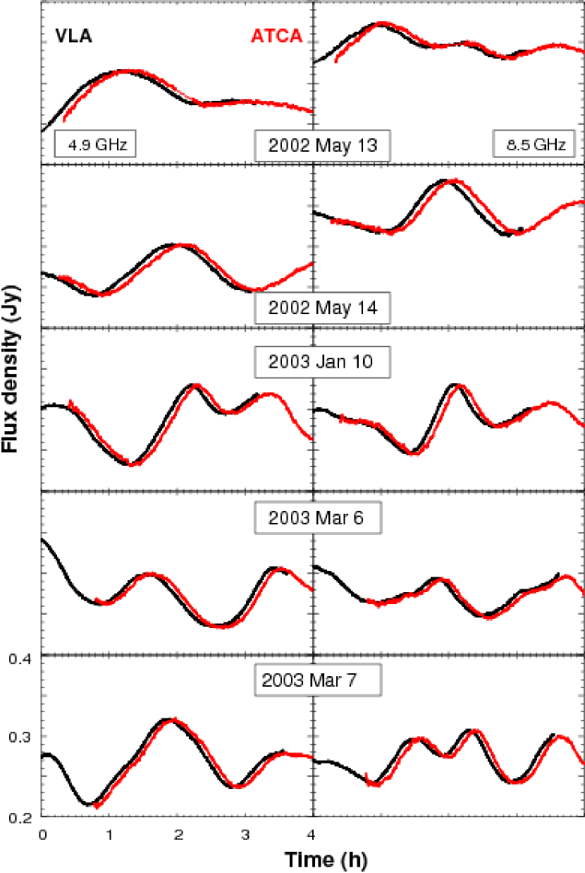
Here we describe the procedure used for data reduction; in §2.3 we estimate the resultant uncertainties in flux density measurement accuracy. Initial data processing was performed using standard tasks in the AIPS and MIRIAD (Sault et al., 1995) software packages. AIPS was used for calibration of the VLA data, and MIRIAD for calibration of the ATCA data. A clear time delay, with the VLA light curves leading those of the ATCA, is evident between the variability patterns seen in Figure 1 at each telescope, and could be seen in the data even before off-line calibration. To measure the delay accurately, antenna gains including pointing- and time-dependent errors were determined for both telescopes at 15 minute intervals using the calibration source PKS 1255$-$316.

For the VLA data, initial gain curves are applied before solving for additional gain or opacity changes using PKS 1255$-$316. For the ATCA, we did not apply gain-elevation corrections separately but solved for all effective gain changes simultaneously assuming a constant flux density for PKS 1255$-$316. For both telescopes, antenna gains vary over the course of the observations by a total of typically 3% at 8.5 GHz and $\sim 1.5$% at 4.9 GHz – here we lump together effects of opacity, pointing and gain-elevation changes as contributing to the overall effective “gain” variations. These variations appear to be tracked very well by the calibration source observations at 15-minute intervals, as outlined below in §2.3. The flux density of PKS 1255$-$316 was determined from the ATCA data and set to be identical at both telescopes. In 2002 May the measured flux densities of PKS 1255$-$316 were 2.4 Jy at 4.9 GHz and 2.3 Jy at 8.5 GHz, which decreased to 2.2 Jy at 4.9 GHz and 1.9 Jy at 8.5 GHz in 2003 March. The ATCA flux density scale is tied to the primary calibrator PKS 1934$-$638. However it is the accuracy of the relative calibration between the two telescopes which is the principal concern for this experiment, rather than the overall flux density scale.

Figure 1: Simultaneous observations of PKS 1257$-$326 at the VLA and ATCA on 5 different days. 4.9 GHz data are shown on the left and 8.5 GHz data on the right. All plots are on the same scale, showing a 4-hour time range, and flux density range from 0.2 to 0.4 Jy. The time ranges shown are 05–09h UT for the data from May, 13–17h UT for the January data, and 09–13h UT for the March data. The flux densities are measured from the visibilities averaged over all baselines of each array, and are plotted here after boxcar smoothing with a width of 50 s. The data were calibrated using observations of the nearby compact source PKS 1255$-$316, and a model of arcsecond-scale extended structure has been subtracted from each of the PKS 1257$-$326 datasets.

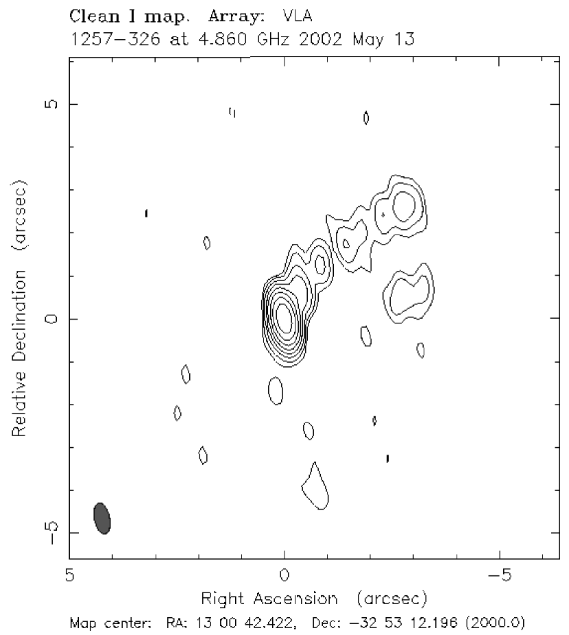
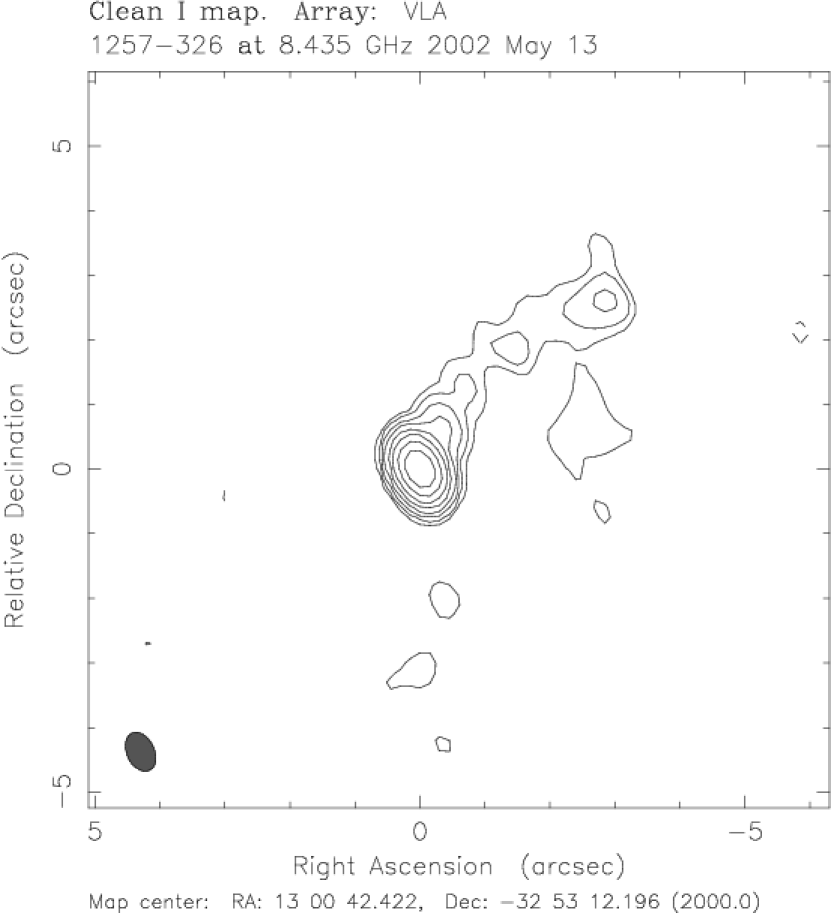
At 4.9 GHz 5% of the total flux density of PKS 1257$-$326 is contained in steep-spectrum components extended over several arcseconds to the north-west of the core, with a broad component offset to the south of the main jet. The same structure is also seen at 8.5 GHz, as shown in the VLA images in Figure 2. In order to accurately compare the flux densities of the scintillating component measured at both telescopes, it is necessary to subtract the contribution of the extended emission, which varies with changing $(u,v)$ coverage for each baseline of each array. We made images of PKS 1257$-$326 from the VLA data obtained during 2002 May, using the Difmap software package (Shepherd, 1997). The VLA at this time was in reconfiguration between the “A” and “BnA” configurations, which provided the highest resolution images. The scintillation in PKS 1257$-$326 is sufficiently rapid to introduce artefacts into an image made from a typical synthesis observation. The VLA has good, two-dimensional instantaneous $(u,v)$ coverage compared with the linear East-West ATCA configuration, allowing an excellent model of the source to be obtained from a single VLA scan of a few minutes. Deeper images of the extended structure were made using 4 hours of VLA data from each subarray, after first subtracting a point source model of variable flux density from each 30 seconds of the data in the visibility domain; the resultant images are displayed in Figure 2.

Figure 2: Images showing the arcsecond-scale extended structure in PKS 1257$-$326, made from VLA data after subtraction of a time-variable point source model from the $(u,v)$ data at both 4.9 and 8.5 GHz. In each case the subtracted flux density was the variable part plus the core such that the resulting map peak is 50 mJy/beam, with contours shown here at $-1,1,2,4,...128\times 0.2$ mJy/beam at both frequencies. In the 8.5 GHz map displayed here, long baselines have been weighted down with $(u,v)$ tapering in order to show clearly the similarity of the unusual extended structure at both frequencies. At each frequency a model of the extended structure (i.e. clean components outside the brightest pixel) was subtracted from all the original calibrated $(u,v)$ data, in order to accurately compare the flux density of the scintillating “core” component measured at each array.

The resultant model clean components, except for the central bright point source component, were subtracted from the PKS 1257$-$326 visibilities for both telescopes, using AIPS task uvsub. This corresponded to a total of 16 mJy being subtracted from the 4.9 GHz data, and 7 mJy from the 8.5 GHz data. The resultant visibilities thus represent only the component which is unresolved at both telescopes, which contains the scintillating component. For all datasets, the data after subtraction of the model are consistent with a point source, and we can conclude that our VLA images are not missing any significant larger scale source structure. The resultant visibilities were written to FITS files and then read into MIRIAD, at which time a decrement of 32 seconds was applied to the VLA data time stamps to convert from IAT to UTC. Flux densities, averaged over the frequency band and over all baselines for each telescope, were then written out as a function of UT for further analysis, along with the rms scatter about the mean for each data point. At this stage no further time averaging was applied beyond the integration times used by each telescope’s real-time correlator, 3.3 s at the VLA and 10 s at the ATCA. The effect of smoothing and interpolation using a range of time intervals was tested later in the time delay fitting process described in §3.

2.3 Flux density measurement uncertainties

If each array sees an identical scintillation pattern, then the expected rms difference $\sigma_{\rm diff}$ between flux density measurements at each array, after correcting for the time delay, is a combination of effects of antenna amplitude gain errors, a contribution $x$ mJy due to errors in the model of extended structure, and the thermal noise for each array $\epsilon$ mJy. Antenna gain errors contribute an overall uncertainty which is a fraction of the total flux density, $gS$. The various errors for each array are independent and hence add in quadrature. Thus

$$\sigma^{2}_{\rm diff}=\sigma^{2}_{\rm V}+\sigma^{2}_{\rm A}=\epsilon_{\rm V}^{2}+\epsilon_{\rm A}^{2}+(g_{\rm V}S)^{2}+(g_{\rm A}S)^{2}+2x^{2},$$ (1)

where the subscripts V and A denote errors for the VLA and ATCA respectively.

Based on the amplitude gain corrections found for the calibration source PKS 1255$-$316, we estimate that our calibration procedure is sufficient to calibrate the target source visibility amplitudes averaged over all baselines to an accuracy of $g\sim 0.1$% at 4.9 GHz and $g\sim 0.25$% at 8.5 GHz at both telescopes, where the flux density scale is tied to PKS 1255$-$316. Errors in the subtracted model, and their effect on the averaged visibilities for the various array configurations, are difficult to quantify, but based on map residuals we estimate that these contribute $x\sim 0.5$ mJy to the overall uncertainties. For an averaging interval of 50 s, corresponding to our chosen smoothing interval for the final fits, the rms scatter due to thermal noise is typically 0.45 mJy for the VLA, and 1.0 mJy for the ATCA, at both frequencies and for all observed epochs. For both arrays, having Cassegrain-focus antennas, the system temperature, and hence the rms measurement noise, increases toward low elevations, as do the fractional errors due to opacity and gain-elevation effects. As each array points toward lower elevations at opposite ends of the observation, the overall uncertainties are relatively constant, with the measurement accuracy being slightly higher in the middle of the observation.

At 4.9 GHz the expected contribution of measurement errors (in mJy) to $\sigma^{2}_{\rm diff}$ for an averaging interval of 50 s and average flux density $\bar{S}\approx 300$ mJy is thus $\sigma^{2}_{\rm diff}{\rm(4.9~{}GHz)}\approx 0.45^{2}+1.0^{2}+2(0.001\bar{S})^{2}+2(0.5^{2})$ giving $\sigma_{\rm diff}\approx 1.4$ mJy. The largest contribution to the errors at 4.9 GHz is the thermal noise in the ATCA data. At 8.5 GHz all error contributions are approximately the same as at 4.9 GHz except for the fractional error term which is estimated to be $2(0.0025\bar{S})^{2}$. Correspondingly, $\sigma_{\rm diff}\approx 1.7$ mJy at the higher frequency for $\bar{S}=300$ mJy and a smoothing interval of 50 s.

3 Results

Figure 1 shows the flux densities of PKS 1257$-$326 measured simultaneously at the ATCA and VLA on the 5 different days at the two frequencies, after subtraction of the model of extended source structure from each dataset. Data are displayed with 50 s boxcar smoothing. The scintillation patterns seen at each telescope appear virtually identical, but clearly displaced in time with the VLA light curve leading that of the ATCA. Data from all epochs and both frequencies show the same effect, with the pattern arriving first at the VLA and then some minutes later at the ATCA.

There are two questions that we wish to address with the present data:

(i) What are the observed time delays and what are their uncertainties?

(ii) How similar are the scintillation patterns seen at the two telescopes?

The measured time delays together with the observed annual cycle data (Paper I) can be used to constrain the properties of the scattering medium and its peculiar velocity. From (ii) we can also determine lower limits on the characteristic length scale of the major axis of the scintillation pattern. In this section we present the results of fitting to the time delay data. §4 presents a combined analysis of the time delay and annual cycle data to determine the scintillation parameters.

The variability patterns can be compared directly to search for any differences by fitting first for a time offset and then subtracting the two patterns. We discuss below the possibility of a small change in the pattern arrival time delay during the course of each observation. However, to begin with, a constant time offset was estimated by minimizing the quantity $\chi^{2}=\sum_{i}[S_{V,i}-S_{A,i}(\Delta t)]^{2}/\sigma_{\rm diff}^{2}$, where trial offsets $\Delta t$ are applied to the ATCA data, and $S_{V,i}$ and $S_{A,i}$ are the VLA and ATCA flux density measurements, respectively, interpolated onto the same grid in time. For each of the 10 datasets, $\Delta t$ was allowed to vary in steps of 1 s between 0 and 1000 s. For the final results presented here we applied boxcar smoothing to the data with a width of 50 s, which corresponds to the interval where the average change in flux density, $\sim 1$ mJy, is approximately equal to the rms measurement noise. A range of different smoothing and sampling intervals for the light curves were tried in order to test the robustness of the fitted time delay. Using a smaller window for smoothing (30 s or 10 s) made no significant difference to the best fit time delay, but resulted in somewhat noisier residuals around the best fit delay. We also tried tests such as dropping low elevation data, e.g. the first and last 20 minutes of each dataset, but this also made essentially no difference to the fitted time delays. This gives us considerable confidence in the robust quality of the data and in our estimation procedures.

Is fitting for a constant time delay the best we can do? The projected VLA-ATCA baseline rotates by almost $20^{\circ}$ from the beginning to the end of the observation. As the baseline is close to one Earth diameter there is little change in projected baseline length over the observations. The time delay will be influenced by the structure of the scintillation pattern and its direction of motion relative to the baseline. One can picture this using the geometry illustrated in Figure 3, where an elliptical scintillation pattern is assumed to represent the average or characteristic scintillation scale. In reality the scintillation pattern is stochastic and it is important to bear in mind that the small sample of the scintillation pattern obtained in a single time delay measurement may not be representative of the average, which was the principle reason for repeating the time delay measurement on consecutive days. We have tested for a change in delay within each observation by splitting the dataset and fitting a delay to each segment, but do not detect any significant differences in delay between subsets. We therefore conclude that fitting a constant time delay for each dataset is justified. However, the assumption of a constant delay is not exactly correct, which will increase the scatter in the residuals to some degree. Moreover, the assumption that the ISM is well characterised by a single velocity may not be strictly correct. Velocity structure in the medium would cause some decorrelation in the pattern as it drifts, and hence would increase the residual differences.

For the case of J1819+3845 (Dennett-Thorpe & de Bruyn, 2002), a large change and reversal in sign of the time delay was seen over the course of the two simultaneous VLA/WSRT observations of this source, due to the large angle through which the projected baseline rotated. For PKS 1257$-$326 we observed at different times of the year in order to measure the time delay for different projections of the scintillation velocity along the baseline.

Figure 3: Sketch illustrating the geometry of the time delay model (not to scale, but the illustrated anisotropy, angles and velocities shown are approximately consistent with our preferred solution). The ellipses represent contours of constant intensity in the scintillation pattern, assumed to be “frozen-in” over a timescale of at least several minutes. Arrows indicate the direction of the velocity v at which the scintillation pattern passes over the telescopes for each observed epoch. The straight dashed lines show the cut through the scintillation pattern observed at each telescope for the direction of ${\bf v}_{\rm Mar}$ shown.

For the final time delay fitting we used a 50 s averaging interval, giving approximately 180 independent time intervals in the $\sim 2.5$ hours of data overlap. We have also performed the fitting after normalizing the flux densities by their mean values in the overlapping time range. Normalizing effectively removes constant fractional errors. Small calibration offsets on the level of a few tenths of a percent were found in some datasets – in particular the March 8.5 GHz data – after processing. Using either the measured flux densities or the flux densities normalized by the mean makes no significant difference to the best fit time delays or their uncertainties. However, using the flux density errors estimated in §2.3, the minimum $\chi^{2}$ values in all cases indicate a poor fit of the model to the data. The larger $\chi^{2}$ values at 8.5 GHz suggest that atmospheric effects may add to the uncertainties such that $\sigma_{\rm diff}$ is slightly underestimated for most datasets. Alternatively, additional pattern differences may also result from either or both of (i) spatial decorrelation resulting from each telescope seeing a different part of the pattern, since the velocity has a component perpendicular to the baseline, or (ii) some temporal rearrangement of the pattern on the timescale of the delay, or equivalently, decorrelation resulting from velocity structure in the medium, so that the observations are not well modeled by a single time delay.

Despite the large values, $\chi^{2}$ in all cases has a well-defined minimum, and therefore we have assumed it is valid to estimate the errors from the change in $\chi^{2}$ about its minimum. We calculate 1$\sigma$ uncertainties using the standard definition. The errors determined this way are approximately consistent with the internal scatter for the epochs which have four datasets (March and May). The similarity of the time delays on consecutive days gives us confidence that the measured delay from each observation is representative of the overall scintillation parameters, despite the small number of maxima and minima observed in each dataset. Also, we have combined the data to estimate a single value for the time delay in each epoch. Table 1 shows all best fit values of $\Delta t$, along with estimated 1$\sigma$ errors.

Table 1: Best fit time delays and correlation coefficients

Obs date	$\Delta t_{4.9}$	$\sigma_{4.9}$	$\chi^{2}_{4.9}$	$\rho_{4.9}$	$\Delta t_{8.5}$	$\sigma_{8.5}$	$\chi^{2}_{8.5}$	$\rho_{8.5}$
	(s)	(s)			(s)	(s)
2002 May 13	495	20	1.16	0.99936(30)	496	27	1.40	0.99638(50)
2002 May 14	468	19	1.55	0.99863(20)	475	24	2.05	0.99591(40)
May combined:  $\Delta t$ = 483 $\pm$ 15 s,  $\chi^{2}$ = 1.56
2003 Jan 10	340	12	1.20	0.99979(05)	330	15	1.55	0.99872(15)
Jan combined:  $\Delta t$ = 333 $\pm$ 12 s,   $\chi^{2}$ = 1.38
2003 Mar 06	333	14	1.10	0.99944(10)	305	24	1.10	0.99951(50)
2003 Mar 07	313	10	1.12	0.99977(05)	314	14	1.58	0.99897(04)
Mar combined:  $\Delta t$ = 318 $\pm$ 10 s,  $\chi^{2}$ = 1.24

Note. — Time delays $\Delta t$ and uncertainties $\sigma$ at each frequency are given, along with minimum reduced $\chi^{2}$ values and correlation coefficients, $\rho$, for the delay-corrected data as discussed in §3. Uncertainties in the last two digits of $\rho$ are indicated in parentheses. The $\chi^{2}$ for each dataset has typically 180 degrees of freedom. Fits to the combined data from each epoch are also given.

The rms scatter in the delayed-difference distributions is generally not much larger than expected due to measurement uncertainties, however there is some noticeable variation between different epochs, with the difference light curves from May showing larger scatter than the other epochs.

In order to address the question of whether there is any decorrelation of the scintillation pattern between the two telescopes, we have calculated the linear Pearson correlation coefficient, $\rho$, for each of the datasets after correcting for the best-fit delay. We have also corrected $\rho$ for the instrumental noise. In all cases $\rho>0.995$ after applying the time delay correction, while the values before correcting for the delay range between 0.91 and 0.97. Values of $\rho$ for the delay-corrected data are shown in Table 1. These were calculated after applying 90 s boxcar smoothing to the data. For both days of observation in May, the correlation coefficients at each frequency are somewhat lower than for the other epochs. This effect is more significant at the higher frequency. As discussed in §4, a larger decorrelation in May would be expected based on the geometry of annual cycle for PKS 1257$-$326.

We have considered the possibility that a larger decorrelation in May might be due to the change in time delay over the course of the observation producing a larger variance in the residual data from this epoch. Our models imply the time delay may change by up to $\sim 10$% over the course of the observation due to baseline rotation. As a check we repeated the calculation after applying the predicted time delays for every 10 minutes of data using models from §4 rather than a constant time delay. However this made no significant difference to the statistics of the residuals or the correlation coefficients.

From Figure 3 it can be inferred that when the scintillation velocity is exactly parallel to the baseline, both telescopes will see an identical pattern provided there is no temporal decorrelation of the pattern on the timescale of the delay. Alternatively, any difference between the patterns seen in this case would be evidence of temporal decorrelation, which would most likely be a result of velocity shear in the ISM. The fact that the time delays are well determined to an accuracy of 3–5% implies that the amount of velocity shear in the scattering medium is not significant on this level. When the pattern drifts at some angle to the baseline, then the second telescope sees a part of the pattern displaced with respect to the first, as illustrated by the straight dashed lines in Figure 3. The amount of spatial decorrelation is also influenced by the degree of anisotropy in the pattern and the angle between the scintillation velocity and the direction of anisotropy. This has been taken into account in the analysis presented in §4.

Finally, it is worth noting that through these accurate flux density and time delay measurements, we can state that PKS 1257$-$326 shows no intrinsic variations at either frequency greater than $\sim 2$ mJy rms on a timescale of 2.5 hours. The time delay observations are of course not sensitive to variations on a timescale longer than the overlap period.

3.1 Annual cycle in characteristic timescale

In Paper I we presented measurements of the characteristic timescale of variability for PKS 1257$-$326 from 2001 and early 2002. From continued ATCA monitoring of the source we now have a number of additional measurements of characteristic timescale, $t_{\rm scint}$. For the present paper, we have reanalysed all data, taking $t_{\rm scint}$ to be the half-width at $1/e$ of the intensity autocorrelation functions. Note that this is slightly different from the half-width at half-maximum definition used in Paper I. Furthermore, we have recomputed the estimates of error in $t_{\rm scint}$, using the formulation given in Appendix A of Rickett et al. (2002) to compute estimation errors in the autocorrelations. Note that this reanalysis makes no significant difference to any of the results presented in Paper I. The updated measurements of $t_{\rm scint}$ are used and shown in the following analysis section.

4 Analysis

The time delay results can be combined with the annual cycle observed in the variability timescale of PKS 1257$-$326 to determine both the scintillation velocity and the dimensions of the scintillation pattern.

The scintillation pattern is assumed to be elliptical with minor axis scale length $a_{\rm min}=s_{0}/\sqrt{R}$ and major axis scale $a_{\rm maj}=s_{0}\sqrt{R}$, and is oriented along the vector $\hat{\bf S}=(\cos\beta,\sin\beta)$. The scintillation velocity is written in the form ${\bf v}(T)=v_{\rm ISS}-v_{\oplus}(T)\equiv(v_{\alpha}(T),v_{\delta}(T))$, and varies on an annual cycle as a function of time, $T$, due to Earth’s orbital motion (Macquart & Jauncey, 2002). Here we define $v_{\oplus}(T)$ as the velocity of the Earth with respect to the solar system barycenter. In this notation, the time delay expected between two telescopes displaced by a distance ${\bf r}=(r_{\alpha},r_{\delta})$ is (Coles & Kaufman, 1978),

$$\Delta t=\frac{{\bf r}\cdot{\bf v}+(R^{2}-1)({\bf r}\times\hat{\bf S})({\bf v}\times\hat{\bf S})}{v^{2}+(R^{2}-1)({\bf v}\times\hat{\bf S})^{2}},$$ (2)

where the dependence of ${\bf v}$ on $T$ is suppressed. The scintillation timescale is

$$t_{\rm scint}=\frac{\sqrt{R}s_{0}}{\sqrt{v^{2}+(R^{2}-1)({\bf v}\times\hat{\bf S})^{2}}}.$$ (3)

In practice neither the variability timescale nor the time delay experiment datasets suffice to uniquely determine all five scintillation parameters, $v_{{\rm ISS},\alpha},v_{{\rm ISS},\delta},\beta,R$ and $s_{0}$, at any one observing frequency, so we fit to both the time delay and the annual cycle data simultaneously. We also fit both frequencies simultaneously, which imposes the additional constraint that the scintillation velocity is identical at the two frequencies; the anisotropic ratios of the scintillation patterns and their associated position angles at the two frequencies are still assumed independent.

Our fit minimises the function

$$\chi^{2}=\chi_{\rm\Delta t}^{2}+\chi_{\rm t_{\rm scint}}^{2},$$ (4)

where $\chi_{t_{\rm scint}}^{2}$ compares our $N_{t_{\rm scint}}=51$ annual cycle measurements, $m_{t_{\rm scint}}(T,\lambda)$, to a model, $M_{t_{\rm scint}}(T,\lambda)$, based on equation (3)

$$\chi_{t_{\rm scint}}^{2}=\frac{1}{N_{t_{\rm scint}}}\sum_{\lambda}\sum_{\rm T}\frac{\left[m_{t_{\rm scint}}(T,\lambda)-M_{t_{\rm scint}}(T,\lambda)\right]^{2}}{\sigma_{t_{\rm scint}}^{2}(T,\lambda)}.$$ (5)

The value of $\chi_{\Delta t}^{2}$ compares our $N_{\Delta t}=3$ time delay measurements, $m_{\Delta t}(T,\lambda)$, to a model, $M_{\Delta t}(T,\lambda)$, based on equation (2),

$$\chi_{\Delta t}^{2}=\frac{1}{N_{\Delta t}}\sum_{\lambda}\sum_{\rm T}\frac{\left[m_{\Delta t}(T,\lambda)-M_{\Delta t}(T,\lambda)\right]^{2}}{\sigma_{\Delta t}^{2}(T,\lambda)},$$ (6)

We have fitted only to the mean time delay from each observation, and have not attempted to model the change in time delay due to the change in telescope baseline during the course of the experiment. As discussed above in §3 we do not detect any significant change in delay over the course of each observation.

The two contributions to $\chi^{2}$, $\chi_{t_{\rm scint}}^{2}$ and $\chi_{\Delta t}^{2}$ are assumed independent, and are weighted so that the relatively few time delay experiments are given equal importance in the fit relative to the annual cycle.

In principle, this fitting procedure allows one to uniquely derive the properties of the scintillation pattern and the peculiar velocity of the scattering medium. However, the system becomes degenerate as the anisotropic ratio becomes large. In the limit $R\rightarrow\infty$, the time delay approaches $\Delta t=({\bf r}\times\hat{\bf S})/({\bf v}\times\hat{\bf S})$ and the scintillation timescale approaches $s_{0}/\sqrt{R}({\bf v}\times\hat{\bf S})$. In this limit one can solve for ${\bf v}\times\hat{\bf S}$ and $s_{0}/\sqrt{R}$, but not uniquely for $\beta$, and thus ${\bf v}_{\rm ISS}$. Since the terms associated with anisotropy scale $\propto{\cal O}(R^{2})$ with respect to the isotropic terms in equations (2) and (3), the uniqueness of the solution depends heavily on the anisotropy intrinsic to the scintillation pattern. For $R\gtrsim 5$, there are degenerate solutions for the scintillation velocity, although the scintillation length scale along the minor axis can still be uniquely determined. To decouple the errors we have fit for the major and minor axis scales $a_{\rm maj}$ and $a_{\rm min}$ rather than $s_{0}$ and $R$. A selection of results is shown in Table 2. In this table the position angle of anisotropy is shown in degrees north through east to follow the usual convention of radio image analysis, although the angle $\beta$ is defined east through north.

Table 2: Scintillation parameters from fitting to the combined annual cycle and time delay measurements

			———  4.9 GHz  ———			———  8.5 GHz  ———
	$v_{{\rm ISS},\alpha}$	$v_{{\rm ISS},\delta}$	$a_{\rm min}$	$a_{\rm maj}$	$90-\beta$	$a_{\rm min}$	$a_{\rm maj}$	$90-\beta$	$\chi^{2}$
	(km s-1)	(km s-1)	($10^{4}$ km)	($10^{4}$ km)	${}^{\circ}($N$\rightarrow$E)	($10^{4}$ km)	($10^{4}$ km)	${}^{\circ}($N$\rightarrow$E)	($N_{\rm DOF}$)
(a)	2.59	18.30	6.68	6.68	0	4.23	4.23	0	106
$\sigma$	0.14	0.18	0.07	0.07	fixed	0.08	0.08	fixed	(53)
(b)	$-256$	219	4.24	487	$-52.8$	3.42	190	$-52.6$	1.75
$\sigma$	47	36	0.08	41	0.3	0.06	36	0.3	(46)
(c)	49.2	$-11.5$	4.23	50.8	$-54.8$	3.43	41.2	$-54.6$	1.97
$\sigma$	7.1	5.1	0.08	0.1	0.4	0.06	0.1	0.5	(49)
(d)	16.5	10.7	4.08	20.5	$-54.1$	3.19	500	$-50.0$	3.6
$\sigma$	fixed	fixed	0.07	1.0	0.4	0.05	390	0.3	(48)

Note. — For each solution, error estimates for all parameters are shown beneath the best fit values. The values for the global reduced $\chi^{2}$ and degrees of freedom ($N_{\rm DOF}$) for each fit are shown in the last column. See §4 for discussion.

The time delays and characteristic timescale at 4.9 GHz are plotted as a function of day of year in Figure 4 and Figure 5, respectively. Model predictions of each of the solutions presented in Table 2 are shown along with the observational data points.

Figure 4: Variation of time delay as a function of day of year for the solutions shown in Table 2. Points near DOY 10, 67 and 134 show the measured time delays.

Figure 5: Annual cycle in characteristic timescale, $t_{\rm scint}$, observed in ATCA data at 4.8 GHz (see §3.1). The plotted lines show the model annual cycles for solutions in Table 2.

The annual cycle and time delay measurements were found to be inconsistent with a solution assuming an isotropic scintillation pattern. In particular, there are no solutions for the isotropic case that fit time delays anywhere near as large as those observed in 2002 May and also match the observed “slow-down” in characteristic timescale which peaks around August. With anisotropy allowed, solutions can be obtained which fit the observations well. There are degenerate solutions for the scintillation velocity, however, as $v_{{\rm ISS},\alpha}$ and $v_{{\rm ISS},\delta}$ are strongly correlated. The best fit velocities tend to lie along a straight line in the $(v_{{\rm ISS},\alpha},v_{{\rm ISS},\delta})$ plane. The major axis scale is also poorly constrained by the annual cycle and time delay data alone.

Another observational constraint on $a_{\rm maj}$ comes from the spatial decorrelation of the pattern between the two telescopes. To model the expected decorrelation we assume that the intensity autocorrelation decreases quadratically from unity near the origin, which is a good approximation if the source has a gaussian brightness distribution and source structure determines the size of the scintillation pattern. We find that when the pattern is highly anisotropic and large compared to the baseline $|{\bf r}|$, the degree of cross-correlation of the two observed patterns is approximately

$$\rho({\bf r},\Delta t)=1-\frac{({\bf r}\times{\bf v})^{2}}{a_{\rm maj}^{2}({\bf v}\times\hat{\bf S})^{2}}.$$ (7)

By far the longest time delays were observed in the May epoch, as in May the scintillation velocity has a large component perpendicular to the baseline ${\bf r}$ as well as a large component parallel to the major axis of the scintillation pattern, along $\hat{\bf S}$. This geometry also implies that we would expect to observe the largest decorrelation of the scintillation pattern in May (see Figure 3 and equation 7). Indeed $\rho({\bf r},\Delta t)$ was observed to be somewhat smaller in May than in the other two epochs. Although $\rho$ is dependent on the velocity, the measured values of $\rho$ in any case provide a lower limit on $a_{\rm maj}$. The lower limit is derived from the model which has the smallest component of screen velocity parallel to $a_{\rm maj}$. For a scattering screen moving with the local standard of rest (solution (d) in Table 2), $a_{\rm maj}$ is found to be $\sim 5\times 10^{5}$ km at 4.9 GHz (a factor of 2 smaller at 8.5 GHz, but the measurement errors are smaller at 4.9 GHz). Better fits to the annual cycle data are found for models with somewhat larger velocity components parallel to $a_{\rm maj}$. These larger velocities require an even larger $a_{\rm maj}$, i.e. even more extreme anisotropy in the scintillation pattern. For example, solution (b) in Table 2 implies a characteristic major axis scale of more than $4\times 10^{6}$ km, and solution (c) implies $a_{\rm maj}\approx 1.2\times 10^{6}$ km at 4.9 GHz. If there is a systematic bias in the determination of $\rho$, this should cancel out by taking the ratio of $\rho$ for different epochs in equation 7 above. Determining $a_{\rm maj}$ in this way was found to give essentially the same results as using $\rho$ for the May epoch alone in equation 7. Combining the results with the constraint that $a_{\rm min}=4.2\times 10^{4}$ km at 4.9 GHz implies a lower limit for the pattern axial ratio $R\gtrsim 12$.

As discussed in Paper I, scintillations observed in PKS 1257$-$326 at frequencies of 4.8 GHz and higher are evidently in the weak scattering regime, where the scintillation length scale is set by whichever is the larger of the angular Fresnel scale, $\theta_{\rm F}=\sqrt{c/(2\pi\nu L)}$, and the source angular size. We can relate the Fresnel radius, $r_{\rm F}=L\theta_{\rm F}$, to $a_{\rm min}$, the $1/e$ value of the intensity autocorrelation function along the minor axis, to find upper limits for the screen distance $L$. For a point source and an isotropic scattering screen, $a_{\rm min}$ corresponds to $1.2r_{\rm F}$, yielding a direct measure of $L$. If source structure influences the scintillation pattern, then $a_{\rm min}>1.2r_{\rm F}$, giving an upper limit for $L$. For an anisotropic scattering medium, the $1/e$ decorrelation point asymptotes to $0.78r_{\rm F}$ along the short axis, and the corresponding upper limit for $L$ is given by $a_{\rm min}\geq 0.78r_{\rm F}$. Uncertainties in $L$ derived this way scale as the square of uncertainties in $a_{\rm min}$. From the best fits to the data, $a_{\rm min}$ is well-determined to within $\sim 2$% despite the degeneracies in velocity and pattern axial ratio. At 4.9 GHz, $a_{\rm min}=4.2\pm 0.1\times 10^{4}$ km gives $L\leq 4$ pc if the scattering medium is isotropic. For an anisotropic scattering medium, incorporating the uncertainty in $a_{\rm min}$, this limit becomes $L\leq 10$ pc.

5 Discussion and conclusions

5.1 Anisotropy in the scintillation pattern

Figure 6 shows the scintillation velocity over the course of the year for PKS 1257$-$326 along with a contour of the fitted scintillation pattern projected on the plane of the sky for anisotropic solution (c) in Table 2. Note that in Paper I the geometry (Figure 4 in Paper I) was displayed as if looking down on the Earth whereas in the present paper we show the view looking up at the sky, corresponding to a reflection of the east-west axis. It is interesting to note that the long axis of the scintillation pattern is aligned in a north-west direction. This is close to the direction of the main extended arcsecond-scale jet in the source, and also with the milliarcsecond-scale jet components observed in VLBI data (Bignall et al., in preparation). Rickett et al. (2002) argued that for the case of PKS 0405$-$385 there is strong evidence that the scintillations result from anisotropic scattering in a thin screen. Likewise for PKS 1257$-$326 we observe the same large negative “overshoot” in the light-curve autocorrelations as investigated by Rickett et al. (2002) and shown to be due to anisotropic scattering. However, given the coincidence of position angle, it may be the case for PKS 1257$-$326 that the anisotropy in the scintillation pattern is also partly related to elongation of the source itself. It is possible that if the source were elongated in a different direction, then such large and rapid scintillation might not be observed through the anisotropic scattering screen. Further analysis is required before conclusions can be drawn as to whether the anisotropy is entirely due to the scattering screen, source structure, or a combination of both source and screen.

Figure 6: Scintillation velocity projected onto the plane of the sky, showing the annual variation of the Earth’s velocity with respect to the scattering screen for anisotropic solution (c) in Table 2. Dotted lines show the velocity on the days of the time delay observations. The filled ellipse represents a contour of the best-fit scintillation pattern at 4.9 GHz. The 1-$\sigma$ contour of the best fit solution for $v_{{\rm ISS},\alpha}$ versus $v_{{\rm ISS},\delta}$ is plotted around the best fit velocity. The component of velocity parallel to the long axis of the scintillation pattern is poorly constrained. If the scattering screen were moving with the local standard of rest, the center of the ellipse would be at position marked in the top right-hand corner.

The origin of the anisotropy may be resolved through a detailed analysis of the polarized flux density scintillations which is ongoing. The ATCA observations provide the full set of Stokes parameters, $I$, $Q$, $U$ and $V$. While no significant circular polarization has been detected for PKS 1257$-$326 ($3\sigma$ upper limit $V=0.2$ mJy, or 0.1% of $I$), we detect significant flux density in the linear polarization parameters $Q$ and $U$. If anisotropy is a property of the scattering medium, then the same degree of anisotropy should be present in all Stokes parameters, while if a property of the source, then the linear polarization is not likely to have the same anisotropy as Stokes $I$. Cross-correlations between the various Stokes parameter pairs can also be used to reveal the microarcsecond-scale polarized structure of the source (Macquart & Jauncey, 2002; Rickett et al., 2002). More information on the properties of both source and scatterer can also be obtained through a detailed analysis of light curve structure functions and power spectra – here we have used only the $1/e$ decorrelation timescale to characterise the scintillations.

5.2 Implications for the source

For a scattering screen at $L=10$ pc, the angular scale of the scintillation pattern implies that the angular size of the scintillating component of the source cannot be much larger than $\sim 300$ by 30 $\mu$as at 4.9 GHz (a factor $\sim 1.2$ smaller at 8.5 GHz). Based on the flux density in the unresolved VLBI core, the observed modulation index and also the asymmetry coefficient analysis of Shishov et al. (2005), we estimate that the flux density of the scintillating component is close to 100 mJy at 4.9 GHz. Then the lower limit for the implied brightness temperature of this component is $T_{b}\approx 1.4\times 10^{12}$ K. If the anisotropy is caused purely by the scattering medium and the source is intrinsically circularly symmetric with angular diameter 30 $\mu$as, then the implied brightness temperature becomes a factor of 10 higher. On the other hand, if the scattering screen is in fact closer than 10 pc, this implies a larger angular size and hence lower $T_{b}$ for the source. $T_{b}\sim 10^{13}$ K is still within the range inferred from VLBI observations of other flat-spectrum quasars (e.g. Horiuchi et al., 2004). A Doppler factor of $\sim 10$–20 is implied to reduce the intrinsic brightness temperature below the inverse Compton limit, however the relativistic beaming evidently does not correspond to an expansion of the emitting region. While there has been some slow evolution of the source flux density over three years of monitoring, we observed a repeated annual cycle, and rapid scintillation has been seen every time PKS 1257$-$326 has been observed since 1995, indicating that the compact component is long-lived and relatively stable over at least a decade.

5.3 Implications for the scattering plasma

The MASIV Survey showed that such extreme intra-hour variability (IHV) as observed in PKS 1257$-$326, PKS 0405$-$385 and J1819+3845 is exhibited by $\ll 1$% of compact flat-spectrum radio sources. Combined with the interpretation of the rapid variability as due to scattering in the very local ISM, this suggests that the covering fraction of such nearby scattering plasma is very small. Alternatively, it is possible that a large fraction of sources may be sufficiently scatter-broadened by the more distant ISM to quench the weak scintillations in more nearby scattering plasma. Further investigation of these possibilities and of the local ISM structure inferred from other observations is needed to fully understand the IHV phenomenon. For a transition frequency between strong and weak scattering of $\sim 5$ GHz, as indicated by the observed peak of modulation close to this frequency, and a screen distance of 10 pc, the scattering measure ($SM$) in conventional units of kpc m^-20/3 is found to be $\log SM\sim-2.8$ using equation 17 from Cordes & Lazio (2002).

All three fast scintillators show evidence of highly anisotropic scintillation patterns (Rickett et al., 2002; Dennett-Thorpe & de Bruyn, 2003). Interestingly, highly anisotropic scattering has also been inferred in the interpretation of parabolic arcs observed in the secondary spectra of pulsars (e.g. Walker et al., 2004). Rickett & Coles (2004) discuss the evidence for highly anisotropic plasma turbulence concentrated in relatively thin layers, suggesting filamentary density structures aligned by the local magnetic field. If the scattering occurred in a very extended medium, the magnetic field, and hence anisotropy in the electron density fluctuations, would tend to have different orientations through the scattering medium and thus the scintillation pattern would be expected to be more isotropic.

5.4 Conclusions

We have presented a combined analysis of two-station pattern arrival time delays and annual cycles in the scintillation timescale for the quasar PKS 1257$-$326. This is the first time such a combined fitting method has been applied to data on a scintillating quasar. We conclude that:

• the large, rapid flux density variations observed in PKS 1257$-$326 are entirely due to interstellar scintillation.

• the scattering occurs in a confined region within 10 pc of the solar system.

The scintillation velocity and geometry of the scintillation pattern for PKS 1257$-$326 could not be uniquely determined using the annual cycle data alone (Paper I), although none of the conclusions presented in Paper I are significantly altered by the new results. Analysis of the combined annual cycle and time delay data shows that there is a high degree of anisotropy in the scintillation pattern. The characteristic linear scale of the pattern along its short axis is well determined, as is the position angle along which the scintillation pattern is elongated. The large anisotropy results in a degeneracy in fitting for the scattering screen velocity, with the best fit velocities lying along a line in the $(v_{\alpha},v_{\delta})$ plane. The scintillation scale on the long axis is constrained using measurements of the spatial decorrelation of the pattern between the VLA and ATCA. An axial ratio of at least 12:1 is inferred.

The implied source brightness temperature is high, up to $10^{13}$ K, but not incompatible with brightness temperatures derived from VLBI observations of other compact quasars. Although a compact source is a requirement for ISS to be observed, it seems likely that it is the unusual scattering properties of the local ISM on the line-of-sight to PKS 1257$-$326, rather than an intrinsic property of the source itself, which give rise to the unusually rapid scintillation observed in this case.

Pattern arrival time delays between widely separated telescopes, combined with measurements of the scintillation timescale, provide a powerful method of determining scintillation parameters for quasars which scintillate rapidly. In order to measure such time delays however, a source must vary by a detectable amount (typically of order 1 mJy or more) over a period of order 1 minute. Such variability is observed in very few sources. Another problem is that the scintillation behaviour for some sources is episodic, making it more difficult to coordinate observations involving multiple telescopes. With more sensitive telescopes coming on line in the future, one would expect to find more low flux density rapid scintillators, thus probing scattering on many more lines of sight through the local ISM.

References

- Bignall et al. (2003) Bignall, H. E., Jauncey, D. L., Lovell, J. E. J., Tzioumis, A. K., Kedziora-Chudczer, L., Macquart, J.-P., Tingay, S. J., Rayner, D. P., & Clay, R. W. 2003, ApJ, 585, 653
- Coles & Kaufman (1978) Coles, W. A., & Kaufman, J. J. 1978, Radio Science, 13, 591
- Cordes & Lazio (2002) Cordes, J. M., & Lazio, T. J. W. 2002, astro-ph/0207156
- Dennett-Thorpe & de Bruyn (2000) Dennett-Thorpe, J., & de Bruyn, A. G. 2000, ApJ, 529, L65
- Dennett-Thorpe & de Bruyn (2002) —. 2002, Nature, 415, 57
- Dennett-Thorpe & de Bruyn (2003) —. 2003, A&A, 404, 113
- Horiuchi et al. (2004) Horiuchi, S., Fomalont, E. B., Taylor, W. K. S. A. R., Lovell, J. E. J., Moellenbrock, G. A., Dodson, R., Murata, Y., Hirabayashi, H., Edwards, P. G., Gurvits, L. I., & Shen, Z.-Q. 2004, ApJ, 616, 110
- Jauncey et al. (2000) Jauncey, D. L., Kedziora-Chudczer, L., Macquart, J. P., Lovell, J. E. J., Perley, R. A., Nicolson, G. D., Rayner, D. P., Reynolds, J. E., Tzioumis, A. K., Wieringa, M. H., & Bignall, H. E. 2000, in IAU Symposium, Vol. 205, 84
- Kedziora-Chudczer et al. (1997) Kedziora-Chudczer, L., Jauncey, D. L., Wieringa, M. H., Walker, M. A., Nicolson, G. D., Reynolds, J. E., & Tzioumis, A. K. 1997, ApJ, 490, L9
- Lang & Rickett (1970) Lang, K. R., & Rickett, B. J. 1970, Nature, 225, 528
- Lovell et al. (2003) Lovell, J. E. J., Jauncey, D. L., Bignall, H. E., Kedziora-Chudczer, L., Macquart, J.-P., Rickett, B. J., & Tzioumis, A. K. 2003, AJ, 126, 1699
- Macquart & Jauncey (2002) Macquart, J.-P., & Jauncey, D. L. 2002, ApJ, 572, 786
- Narayan (1992) Narayan, R. 1992, Phil. Trans. R. Soc. Lond. A., 341, 151
- Phillips & Spencer (1955) Phillips, G. J., & Spencer, M. 1955, Proceedings of the Physical Society B, 68, 481
- Rickett & Coles (2004) Rickett, B. J., & Coles, W. A. 2004, Bulletin of the American Astronomical Society, 36, 1539
- Rickett et al. (2002) Rickett, B. J., Kedziora-Chudczer, L., & Jauncey, D. L. 2002, ApJ, 581, 103
- Sault et al. (1995) Sault, R. J., Teuben, P. J., & Wright, M. C. H. 1995, in ASP Conf. Ser. 77: Astronomical Data Analysis Software and Systems IV, 433
- Shepherd (1997) Shepherd, M. C. 1997, in ASP Conf. Ser. 125: Astronomical Data Analysis Software and Systems VI, 77
- Shishov et al. (2005) Shishov, V. I., Smirnova, T. V., & Tyul’Bashev, S. A. 2005, Astronomy Reports, 49, 250
- Walker et al. (2004) Walker, M. A., Melrose, D. B., Stinebring, D. R., & Zhang, C. M. 2004, MNRAS, 354, 43