Empirical Models for Dark Matter Halos. II. Inner profile slopes, dynamical profiles, and $\rho/\sigma^{3}$

Abstract

We have recently shown that both the Prugniel-Simien model and Sérsic’s function (hereafter referred to as the Einasto model when applied to internal density profiles) describe simulated dark matter halos better than an NFW-like model with equal number of parameters. Here we provide analytical expressions for the logarithmic slopes of these models, and compare them with data from real galaxies. Depending on the Einasto parameters of the dark matter halo, one can expect an extrapolated, inner (0.01–1 kpc), logarithmic profile slope ranging from $\sim-0.2$ to $\sim-1.5$, with a typical value at 0.1 kpc around $-0.7$. Application of this (better fitting) model therefore alleviates some of the past disagreement with observations on this issue. We additionally provide useful expressions for the concentration and assorted scale radii: $r_{s},r_{-2},r_{\rm e},R_{\rm e},r_{\rm vir}$, and $r_{\rm max}$ — the radius where the circular velocity profile has its maximum value. We also present the circular velocity profiles and the radial behavior of $\rho(r)/\sigma(r)^{3}$ for both the Einasto and Prugniel-Simien models, where $\sigma(r)$ is the velocity dispersion associated with the density profile $\rho(r)$. We find this representation of the phase-space density profile to be well approximated by a power-law with slope slightly shallower than $-2$ near $r=r_{-2}$.

1 Introduction

In an interesting turn of events, Sérsic’s (1963, 1968) 3-parameter function, developed to describe the projected (on the plane of the sky) radial stellar distributions of galaxies, has been shown to also match the internal (3D) density profiles of simulated dark matter halos (Navarro et al. 2004). Intriguingly, this function was shown to provide a better fit than the 3-parameter NFW-like model with arbitrary inner power-law slope (Diemand, Moore, & Stadel 2004; Merritt et al. 2005, 2006). The functional form of Sérsic’s equation was independently developed by Einasto (1965, 1968, 1969) and used to describe the internal density profiles of galaxies (see also Einasto & Haud 1989 and Tenjes, Haud, & Einasto 1994). We shall therefore refer to this function as the Sérsic model when applied to projected distributions, and as the Einasto model when applied to internal density profiles.

One of the main concerns in (Merritt et al. 2005, 2006) was whether the deprojected form of Sérsic’s function might provide a better description of the density profiles than the Einasto model. Specifically, in Merritt et al. (2006, hereafter Paper I), the analytical approximation to the deprojection of Sérsic’s function given in Prugniel & Simien (1997) was tested along with the Einasto model, the NFW-like model, and various other fitting functions. Overall, the Prugniel-Simien and Einasto models performed the best, providing a good description to both the galaxy- and cluster-sized halos built from hierarchical $N$-body simulations, and also the monolithic cold collapse halos. Curiously, while the Prugniel-Simien model provided the best fit to the cluster-sized halos, Einasto’s model provided a better fit to the galaxy-sized halos. In this paper we explore some of the properties of these two models and some of the consequences they imply, and comparisons they enable, with real galaxies and galaxy clusters.

In an effort to help clarify and unify the various parameters of the different models, Section 2 provides relations between such quantities as effective radius $R_{\rm e}$, virial radius $r_{\rm vir}$, the radius where the logarithmic slope of the model equals $-2$, $r_{-2}$, and ‘concentration’ as measured by observers and by modelers.

In Section 3 we present the phase-space density profiles, or more specifically, the density profiles divided by the cube of their associated velocity dispersion profiles, showing how, for sufficiently large shape parameters $n$, both the Einasto model and the Prugniel-Simien model approximate a power-law $\sim r^{-2}$ near $r_{-2}$.

In Section 4 we derive the logarithmic slopes of the Einasto and Prugniel-Simien model, and compare these with real data. This is of particular interest because the innermost slope of these models is considerably shallower than $-1$ and in fact equal to zero in the case of the Einasto model at $r=0$. The inward extrapolation of these models, rather than the NFW-like model, therefore noticeably reduces the disagreement between modelers and observers on this issue.

Our findings are summarized in Section 5.

2 The models: assorted radial scales and concentration

We will discuss three (3-parameter) empirical models used for describing the internal density profiles of galaxies, clusters, and halos. Each model has three parameters and their application to simulated halos can be seen in Paper I.

The first model is an adaptation of the Navarro, Frenk, & White (1995, hereafter NFW) model to give a double power-law with an outer slope of $-3$ and an arbitrary inner slope denoted by $\gamma$. The radial density profile, $\rho(r)$, of this model can be written as

$$\rho(r)=\frac{2^{3-\gamma}\rho_{s}}{(r/r_{s})^{\gamma}(1+r/r_{s})^{3-\gamma}},$$ (1)

where $r_{s}$ is the scale radius at the density $\rho_{s}$, marking the center of the transition between the inner and outer power-laws with (extrapolated) slopes of $-\gamma$ and $-3$. This function represents a restricted form of the more generic ($\alpha,\beta,\gamma$) model (Hernquist 1990, his equation 43; see also Zhao 1996) and we shall refer to it as the ($1,3,\gamma$) model. Setting ($\alpha,\beta,\gamma$)=(1, 3, 1) yields the NFW model, while (1.5, 3, 1.5) gives the model in Moore et al. (1999). Because the ($1,3,\gamma$) model has already been studied in detail, our main focus will be on the models of Einasto (1965) and Prugniel & Simien (1997).

Einasto’s model is given by the equation

$$\rho(r)=\rho_{\rm e}\exp\left\{-d_{n}\left[(r/r_{\rm e})^{1/n}-1\right]\right\}.$$ (2)

The parameter $n$ describes the shape of the density profile. Larger values of $n$ result in steeper inner profiles and shallower outer profiles. The quantity $d_{n}$ is defined to be a function of $n$ such that $\rho_{\rm e}$ is the density at the effective radius $r_{\rm e}$ which encloses a volume containing half of the total mass. A good approximation for $n\gtrsim 0.5$ is given by $d_{n}\approx 3n-1/3+0.0079/n$ (Mamon 2005, priv comm.), although we have used the exact value coming from $\Gamma(3n)=2\times\gamma(3n,d_{n})$, where $\gamma(x_{1},x_{2})$ and $\Gamma(x)$ are the incomplete and complete gamma functions, respectively (see Paper I). The mass profile (Mamon & Łokas 2005, their equation A2; Cardone et al. 2005, their equation 11) is given by

$$M(r)=4\pi nr_{\rm e}^{3}\rho_{\rm e}{\rm e}^{d_{n}}{d_{n}}^{-3n}\gamma(3n,x).$$ (3)

We shall at times refer to the value of $n$ from Einasto’s model as $n_{\rm Ein}$.

The Prugniel-Simien model can be expressed as

$$\rho(r)=\rho^{\prime}\left({r\over R_{\rm e}}\right)^{-p}\exp\left[-b_{n}\left(r/R_{\rm e}\right)^{1/n}\right],$$ (4)

with

$$\rho^{\prime}={M\over L}\ I_{\rm e}{\rm e}^{b_{n}}\ {b_{n}}^{n(1-p)}\ {\Gamma(2n)\over 2R_{\rm e}\Gamma(n(3-p))}.$$ (5)

Once again, the parameter $n$ describes the curvature of the density profile. The quantity $b_{n}$ is a function of $n$ defined in such a way that $R_{\rm e}$ is the effective radius containing half of the total mass when the 3D sphere defined by this density profile is seen in projection onto a 2D plane. Although we use the exact solution for $b_{n}$, coming from $\Gamma(2n)=2\times\gamma(2n,b_{n})$ (see Graham & Driver 2005), $b_{n}$ can be approximated by $2n-1/3+0.009876/n$ for values of $n\gtrsim 0.5$ (Prugniel & Simien 1997). In addition to $n$ and $R_{\rm e}$, the third parameter which one solves for, $\rho^{\prime}$, is defined so that the volume-integrated mass from equation 4 is equal to the area-integrated mass of a Sérsic function with the standard parameter set $I_{\rm e},R_{\rm e},$ and $n$ (see Paper I).

The final term $p$ is not a parameter but instead, like $b_{n}$, another function of $n$. It is chosen to maximize the agreement between the Prugniel-Simien model and the deprojected Sérsic model having the same parameters $n$ and $R_{\rm e}$. A good match is obtained when $p=1.0-0.6097/n+0.05463/n^{2}$ (Lima Neto et al. 1999; see also Paper I, their figure 13). The value of $p$ is also responsible for determining the logarithmic profile slope at small radii. Setting $p$ to zero, the Prugniel-Simien model has the same functional form as Einasto’s model.

The internal density of the Prugniel-Simien model at $r=R_{\rm e}$ is given by $\rho_{\rm e}=\rho^{\prime}{\rm e}^{-{b_{n}}}$, and the projected surface density at $R=R_{\rm e}$, denoted by $I_{\rm e}$, can be solved for using equation 5. Comparisons of dark matter halos (fitted with the Prugniel-Simien model) with real galaxies (fitted with Sérsic’s model) is obviously remarkably easy using this model. The associated mass profile (Lima Neto et al. 1999; Márquez et al. 2001) is given by the equation

$$M(r)={4\pi n{R_{\rm e}}^{3}}\rho^{\prime}{{b_{n}}^{-(3-p)n}}\gamma\left((3-p)n,Z\right),$$ (6)

where $Z\equiv b_{n}(r/R_{\rm e})^{1/n}$. Expressions for the associated gravitational potential, force, and velocity dispersion can be found in Terzić & Graham 2005). In what follows, we shall at times refer to the value of $n$ from the Prugniel-Simien model as $n_{\rm PS}$.

In the following subsections we explore a number of important radii associated with the above models, and address the issue of ‘concentration’.

2.1 The peak in the $4\pi Gr^{2}\rho(r)$ [km s^-1]² profile, $r_{-2}$

As will be discussed in Section 4, the scale radii $r_{\rm e}$ of the Einasto model, and the (projected) half-mass radii $R_{\rm e}$ from the Prugniel-Simien model, occur where the logarithmic slope of the density profile is $\sim-3$. This can be quite far out, and so we define an additional radial scale. We do so by obtaining the radius where the profile $4\pi Gr^{2}\rho(r)$, which has units of velocity squared, has its maximum. The integral of this profile gives the enclosed mass.

For the (1, 3, $\gamma$) model (equation 1), this maximum occurs at a radius that we denote by $r_{-2,(1,3,\gamma)}$, such that

$$r_{-2,(1,3,\gamma)}=(2-\gamma)r_{s},\hskip 30.0pt\gamma<2.$$ (7)

When $\gamma=1$, as in the NFW model, the radius $r_{-2,(1,3,\gamma)}=r_{s}$, and when $\gamma=1.5$ one has $r_{-2,(1,3,\gamma)}=r_{s}/2$. It turns out that the radius $r_{-2,(1,3,\gamma)}$ corresponds to the point where the logarithmic slope of the (1, 3, $\gamma$) density profile equals $-2$, hence the adopted nomenclature. Similarly for the Einasto and Prugniel-Simien density model, solving where the derivative of the profile $4\pi Gr^{2}\rho(r)$ equals zero, one finds that these profiles also peak at the radius where their logarithmic slope equals $-2$. This is easy to understand when one notes that the solution to ${\rm d}[r^{2}\rho(r)]/{\rm d}r=0$ leads to $d\rho/\rho=-2dr/r$. It is also easy to show that this corresponds to a maximum for any density profile with a monotonically decreasing slope.

For Einasto’s model (equation 2), one has

$$r_{-2,{\rm Ein}}=\left(\frac{2n_{\rm Ein}}{d_{n}}\right)^{n_{\rm Ein}}r_{\rm e},$$ (8)

and for the Prugniel & Simien density profile (equation 4) one has

$$r_{-2,{\rm PS}}=\left(\frac{n_{\rm PS}(2-p)}{b}\right)^{n_{\rm PS}}R_{\rm e}.$$ (9)

When $n_{\rm Ein}=6$, $r_{-2,{\rm Ein}}\sim 0.10r_{\rm e}$. When $n_{\rm PS}=3$, $r_{-2,{\rm PS}}\sim 0.25R_{\rm e}$. (These representative values of the shape parameter have been taken from Paper I, which applied the above models to a number of simulated dark matter halos.)

Evaluating Einasto’s model (equation 2) at $r_{-2,{\rm Ein}}$ to give the density $\rho_{-2,{\rm Ein}}$, and expressing $r_{\rm e}$ in terms of $r_{-2,{\rm Ein}}$ (equation 8), Einasto’s model can be written as

$$\rho_{\rm Ein}(r)=(\rho_{-2,{\rm Ein}})\times\exp\{-2n[(r/r_{-2,{\rm Ein}})^{1/n}-1]\},$$ (10)

where

$$\rho_{-2,{\rm Ein}}=\rho_{\rm e}{\rm e}^{d-2n}.$$ (11)

This is the expression used in Navarro et al. (2004).

Re-expressing Prugniel & Simien’s model in terms of $r_{-2}$, one has

$$\rho_{\rm PS}(r) = (\rho_{-2,{\rm PS}})\left(\frac{r}{r_{-2,{\rm PS}}}\right)^{-p}$$ (12)

$$\hskip-50.0pt\times\exp\{-n(2-p)[(r/r_{-2,{\rm PS}})^{1/n}-1]\},$$

where

$$\rho_{-2,{\rm PS}}=\rho^{\prime}\left(\frac{b}{n(2-p)}\right)^{np}\exp\{n(p-2)\}.$$ (13)

2.2 The peak in the circular velocity profile, $r_{\rm max}$

While an isothermal density profile, $\rho(r)\propto r^{-2}$, has a flat rotation curve, the radius where the logarithmic slope of our (non-isothermal) density profiles equals $-2$, $r_{-2}$, does not coincide with the flat portion of the rotation curve, i.e. where the rotation curve has its maximum value. The rotation curves are simply given by the circular velocity profiles: ${v_{\rm circ}}^{2}(=GM(r)/r)$, with $M(r)$ defined previously. The maximum occurs at a radius $r_{\rm max}$ which is larger than $r_{-2}$, and is shown in Figure 1 as a function of both the effective radius and $r_{-2}$ for the Einasto and Prugniel-Simien models.

Figure 1: Circular velocity profiles for a) the Einasto model (equation 2), and b) Prugniel & Simien’s model (equation 4), for varying values of the profile shape $n$: $n=0.5$ (solid lines), $n=1$ (dotted), $n=2$ (dashed), $n=4$ (dash-dot), $n=10$ (dash-triple dot). The lower panels show the same thing except the radius has been normalized against $r_{-2}$ (the radius where the logarithmic slope of the density profile equals $-2$) rather than the effective radii of the models. Panel c) Einasto’s model, panel d) Prugniel & Simien’s model. $n=0.5$ (solid line); $n=1$ (dotted line); $n=2$ (dashed line); $n=4$ (dot-dash line); $n=10$ (triple-dot-dash line).

The width near the peak of the circular velocity profile increases as the value of $n$ increases. Density profiles with larger values of $n$ will approximate a flat rotation curve over a greater radial extent (in units of $r_{-2}$) than profiles with smaller values of $n$ (Figure 1c and d).

The radius $r_{\rm max}$ can be obtained numerically by solving the expression for when the derivative of $GM(r)/r$ equals zero. For the Einasto model, this amounts to solving

$$\gamma(3n,x)=x^{3n}{\rm e}^{-x}/n,$$ (14)

with $x=d_{n}(r_{\rm max}/r_{\rm e})^{1/n}$. For the Prugniel & Simien model, one needs to solve the expression

$$\gamma(n(3-p),Z)=Z^{n(3-p)}{\rm e}^{-Z}/n,$$ (15)

with $Z=b(r_{\rm max}/R_{\rm e})^{1/n}$. The results are shown in Figure 2, with $r_{\rm max}$ normalized against $r_{-2}$.

Figure 2: The radius where the circular velocity profile peaks, divided by the radius where the logarithmic slope of the density profile equals $-2$, is shown as a function of the density profile shape $n$ for a) the Einasto profile (equation 2), and b) Prugniel & Simien’s profile (equation 4).

When $n=3.6$ (and 2.9) in the Prugniel-Simien model — the average profile shape for our galaxy-sized (and cluster-sized) CDM halos, see Paper I — $r_{\rm max}\sim$ 2.17 $r_{-2}$ (and 2.10 $r_{-2}$). When $n=6$ (and 5.0) in the Einasto model, $r_{\rm max}\sim$ 2.21 $r_{-2}$ (and 2.16 $r_{-2}$). This can be compared with the ($\gamma=1$) NFW model for which $r_{\rm max}$ is known to equal $\sim$ 2.16 $r_{-2}$.

2.3 Concentration and the virial radius, $r_{\rm vir}$

Given the re-newed application of Einasto’s model, which has the same functional form as Sérsic’s model that is used by observers in describing projected distributions, it would seem relevant to inquire if we can also make use of the type of concentration indices that observers use. There are two flavors.

The first is a ratio of two radii. While this may sound qualitatively similar to the NFW concentration, it is in fact fundamentally different. A classical example would be the ratio between the radii containing 50% and 25% of a galaxy’s total light (Fraser 1972). In the case of a universal density profile, with only a radial scale and a density scale, the ratio of radii containing 50% and 25% of the total (asymptotic) mass would always be exactly the same. That is, if we were to use the new concentration index $r_{\rm e}/r_{-2}$, then if $n$ is assumed to be constant (i.e., if a universal profile exists), this ratio will be the same for every profile (see equations 8 and 9). A similar example comes from Butcher & Oemler (1984) who defined a galaxy cluster concentration index $C=\log(R_{60}/R_{20})$, where $R_{x}$ is the radius enclosing $x$% of the galaxies in a cluster.

The second type of concentration index is a ratio of flux, compared to a ratio of radii, within two specified radii (Okamura, Kodaira, & Watanabe 1984). An example is the flux within the radius containing half an object’s total light divided by the flux within one third of this radius (Trujillo, Graham, & Caon 2001). But again, if the density profiles are universal, then such concentration indices will always have the same value. It is because real galaxies do not have universal light-profiles, i.e. a range of Sérsic ($R^{1/n}$) indices are observed, that such concentrations indices work.

Abraham et al. (1994) used a galaxy concentration index defined as the ratio of flux within the radius containing an object’s total light (rather than half its light) divided by the flux within 1/3 of this radius. Now because, in general, galaxies do not have well-defined edges but rather their light slowly peters out into the noise of the sky-background flux, deeper and deeper exposures yield increasingly larger total radii, and a flux ratio that tends to 1 for every galaxy. But because of the limited aperture sizes Abraham et al. (1994) used to define the total galaxy light, they obtained values different than 1. The quantity they measured was thus a function of not only the light-profile shape, but how many $R_{\rm e}$ they sampled in their largest aperture, as discussed in Graham, Trujillo, & Caon (2001).

In a somewhat similar manner, the NFW concentration works because it too is dependent on the background noise, specifically, the mean matter density of the universe. The virial radius, $r_{\rm vir}$, is used to quantify the density of dark matter halos relative to the background. It is defined as the radius of a sphere containing an average matter density that is some specific number greater than the mean matter density in the universe. In Paper I we reported that our simulated halo profiles were computed using a value of 368. It is however common to also see a value of $\sim$337 when $\Omega_{\rm baryon}=0.3,\Omega_{\Lambda}=0.7$, and $h=0.7$ (e.g., Bryan & Norman 1998). Before the cosmological constant became fashionable, a value of $\sim$178 was used for the flat Einstein de Sitter universe.

Using equations 3 and 6 for the mass profile, one can (numerically) solve the following expression to obtain the virial radius in units of the scale radius $r_{\rm e}$ and $R_{\rm e}$ from the Einasto and Prugniel-Simien model, respectively.

$$3M(r_{\rm vir})/(4\pi{r_{\rm vir}}^{3})=337\langle\rho_{\rm universe}\rangle.$$ (16)

Halos do of course extend beyond $r_{\rm vir}$ (e.g., Macció, Murante, & Bonometto 2003; Prada et al. 2005). The results are shown in the top panels of Figure 3, where one can see how the virial radius is monotonically related to the density contrast between $\rho_{\rm e}$ and $\langle\rho_{\rm universe}\rangle$. As $r_{\rm vir}$ increases beyond the effective radius, the incomplete gamma function in the mass profiles starts to asymptote to a constant value and the slope in the figures tends to 1/3.

Figure 3: Panels a) and b) show the virial radius (normalized against the effective radius $r_{\rm e}$ and $R_{\rm e}$, respectively), as a function of the scale-density $\rho_{\rm e}$ relative to the average background density of the universe for Einasto’s model (equation 2) and the Prugniel-Simien model (equation 4), respectively. Panels c) and d) are similar to panels a) and b) but with the virial radius normalized by the radius where the logarithmic slope of the density profile equals $-2$. Panels e) and f) show the associated, negative, logarithmic slope of the density profile at the virial radius, denoted by $\gamma_{\rm vir}$. $n=0.5$ (solid line); $n=1$ (dotted line); $n=2$ (dashed line); $n=4$ (dot-dash line); $n=10$ (triple-dot-dash line).

From the relations connecting $r_{\rm e}$ and $R_{\rm e}$ with $r_{-2}$ (equations 8 and 9), one can obtain the virial radius in units of $r_{-2}$. This is shown in the middle panels of Figure 3. The ratio $r_{\rm vir}/r_{-2}$ is referred to by modelers as the concentration parameter. It does not refer to the curvature or shape of the profiles, as observers might initially think, but is a measure of the density contrast of the halo relative to the average background density of the universe. Obviously, if one did not wish to use the virial radius (see Macciò, Murante, & Bonometto 2003 for an alternative prescription), then a similar ‘concentration parameter’ can be defined in terms of $\rho_{\rm e}/\langle\rho_{\rm universe}\rangle$. The slope at $r=r_{\rm vir}$ is shown in the lower panels of Figure 3 as a function of $\rho_{\rm e}/\langle\rho_{\rm universe}\rangle$.

If one thinks of dark matter halos as icebergs, which can be lowered and raised relative to the background density of the universe, then profile universality means that one can use the offset between $\langle\rho_{\rm universe}\rangle$ and either $\rho_{e}$ or $\rho_{-2}$ or $\rho^{\prime}$ as a measure of ‘concentration’. But if a range of profile shapes exists, i.e. different $n$ ($\alpha$ in the notation of Navarro et al. 2004), the difference between $\rho_{e}$ and $\rho_{-2}$ and $\rho^{\prime}$ will depend on the profile shape. What this means is that the concentration one measures will depend on where one samples the halo’s density. This is important because the halo density is thought to reflect the mean density of the universe when the halo formed, and is thus a measure of the collapse redshift of the halo.

It would be of value to explore whether or not the use of $\rho_{\rm e}$ and $M(r_{\rm e})$ (and $M(R_{\rm e})$ in the case of the Prugniel-Simien model), rather than $\rho_{-2}$ and $M_{\rm vir}$ may account for some of the scatter in diagrams plotting concentration versus halo mass, or equivalently, scale radius versus scale density.

Finally, we note that the use of a Petrosian-style radius (Petrosian 1976; Graham et al. 2005), such that the mean density inside of some radius divided by the density at that radius equals some constant value, is not suitable in the case of structural homology. This is because such a radius will be equal to the same fractional number of scale radii ($r_{\rm e}$ or $r_{-2}$) for every halo. That is, a Petrosian-like radius will just be a re-expression of the scale radius.

3 On the power-law nature of $\rho/{\sigma}^{3}$

There has been recent interest in the the pseudo phase-space density profiles represented by $\rho(r)/{\sigma(r)}^{3}$. This quantity appears to be well approximated by a power-law $r^{-\alpha}$, with $\alpha\approx 1.94$ (Taylor & Navarro 2001; Ascasibar et al. 2004; Rasia, Tormen, & Moscardini 2004; Sota et al. 2006; Barnes et al. 2006). Independently of any model, Dehnen & McLaughlin (2005) found a best-fit value of $\alpha=1.92\pm 0.01$ using the halos A09-F09 and G00-G03, which we studied in Paper I.

Figure 4 shows the ratio $\rho(r)/{\sigma(r)}^{3}$ for the Prugniel-Simien density profile (equation 4) coupled with its spatial (i.e., not projected) velocity dispersion profile given in Terzić & Graham (2005, their equation 28). Isotropy in velocity space has been assumed. As can be seen, the profiles are not exactly featureless power-laws, but for $n\gtrsim 4$ the departure from a power-law, over the radial range shown, is less than about 20%.

Figure 4: Prugniel-Simien density profile $\rho(r)$ (equation 12) divided by the cube of its spatial (i.e., not projected) velocity dispersion profile $\sigma_{s}(r)$ (Terzić & Graham 2005, their equation 28). The curves are such that: $n=0.5$ (solid line), $n=1$ (dotted), $n=2$ (short-dashed), $n=4$ (dash-dot), $n=10$ (long-dash). The curves asymptotically approach a line having slope $-2$ (shown by the solid straight line) as $n\rightarrow\infty$. One obtains the same asymptotic behavior using the projected velocity dispersion profile. The lower panel shows the difference between the curved profiles and the line of slope $-2$, divided by the density of the curved profiles.

For the Einasto density profile (equation 10), the spatial velocity dispersion profile can be obtained by integrating the isotropic Jeans equation of hydrostatic equilibrium

$${\sigma_{\rm s}}^{2}(r)={G\over{\rho(r)}}\int_{r}^{\infty}\rho({\bar{r}}){{M({\bar{r}})}\over{\bar{r}}^{2}}{\rm d}{\bar{r}}.$$ (17)

Expressing $r_{\rm e}$ in terms of $r_{-2}$ (equation 8) in the mass profile $M(r)$ (equation 3), one obtains

$${\sigma_{\rm s}}^{2}(x) = \frac{GM_{\rm tot}}{r_{-2}}\frac{(2n)^{1+n}}{2}\frac{{\rm e}^{x}}{\Gamma(3n)}$$ (18)

$$\hskip-20.0pt\times\int_{x}^{\infty}{\bar{x}}^{-n-1}{\rm e}^{-{\bar{x}}}\gamma\left(3n,{\bar{x}}\right){\rm d}{\bar{x}},$$

where ${\bar{x}}=d_{n}({\bar{r}}/r_{\rm e})^{1/n}=2n({\bar{r}}/r_{-2})^{1/n}$. Integration to infinity for this expression is avoided by making the substitution ${\bar{x}}=(x/\cos\theta)$, such that ${\rm d}{\bar{x}}/{\rm d}\theta=x\sin\theta/\cos^{2}\theta$, giving

$${\sigma_{\rm s}}^{2}(x) = \frac{GM_{\rm tot}}{r_{-2}}\frac{(2n)^{1+n}}{2}\frac{{\rm e}^{x}x^{-n}}{\Gamma(3n)}$$ (19)

$$\hskip-70.0pt\times\int_{0}^{\pi/2}\tan\theta\cos^{n}\theta\hskip 3.0pt{\rm e}^{-x/\cos\theta}\hskip 2.0pt\gamma\left(3n,\frac{x}{\cos\theta}\right){\rm d}\theta.$$

Figure 5 shows $\rho/{\sigma_{s}}^{3}$ for the Einasto density profile.

Figure 5: Same as figure 4 except that Einasto’s density profile (equation 10) has been used here.

From the residual profiles in Figures 4 and 5, one can see that, over the radial range $0.1<r/r_{-2}<10$, a slightly shallower slope than $-2$ exists for $4<n<10$ (Einasto case, Figure 5) and $2<n<10$ (Prugniel-Simien case, Figure 4). Although at $r=r_{-2},-{\rm d}\log\rho/{\rm d}\log r\equiv\gamma=2$, for $n_{\rm Ein}=6,\gamma_{\rm Ein}(0.1r_{-2})=1.36$ and $\gamma_{\rm Ein}(10r_{-2})=2.94$, and for $n_{\rm PS}=3,\gamma_{\rm PS}(0.1r_{-2})=1.62$ and $\gamma_{\rm PS}(10r_{-2})=2.56$. The slope of the density profile does therefore change over this radial range. This can be appreciated in Figures 6 and 7 which show the negative, logarithmic slope of the (cube of the) velocity dispersion profile, the density profile, and $\rho/{\sigma_{s}}^{3}$. For large values of $n$, $\rho/{\sigma_{s}}^{3}\approx r^{-2}$.

Figure 6: Negative, logarithmic slopes associated with the Prugniel-Simien model (equation 12). The curves in the lower panel equal the curves in the middle panel minus those in the upper panel. See section 3 for details.

Figure 7: Same as figure 6 except that Einasto’s density profile (equation 10) has been used here.

4 Density profile slopes

De Blok (2005) has argued that the inner profile slopes of simulated, dark matter halos are inconsistent with observations of dark matter dominated galaxies (Moore et al. 1999; Salucci & Burkert 2000; Marchesini et al. 2002; de Blok, Bosma, & McGaugh 2003; Gentile et al. 2006; Goerdt et al. 2006). He reports that the inner density profiles of low surface brightness (LSB) galaxies have logarithmic slopes significantly shallower than $-1$ at a radius of 0.4 kpc. This is important because it suggests a possible problem with hierarchical $\Lambda$CDM simulations of dark matter halos, which, at least from (1, 3, $\gamma$) model fits, typically have inner slopes steeper than $-1$.

While there is presently no consensus as to why such a disagreement exists, some of the apparent discrepancy may arise from either baryonic processes which modify the dark matter profile (e.g., Mashchenko, Couchman, & Wadsley 2006), or from systematic biases in measuring inner slopes from HI and H$\alpha$ long-slit observations (van den Bosch et al. 2000; Swaters et al. 2003a; Spekkens, Giovanelli, & Haynes 2005, but see de Blok 2003). For example, non-circular motions can make galaxies appear less cuspy than they really are. Significant, in the sense of non-zero, non-circular motions are indeed present in many LSB galaxies where high resolution 2D velocity fields are available (e.g., Swaters et al. 2003b; Blais-Ouellette et al. 2004; Coccato et al. 2004; Simon et al. 2005). However, on their own, these do not explain the observed difference in slope (de Blok et al. 2003; Gentile et al. 2006). But in combination with gas pressure support and projection effects, Valenzuela et al. (2005) argue that this may account for the relatively shallow slopes in observations. Using extensive simulations of observing and data processing techniques, Spekkens et al. (2005) also report how measurements from long-slit, optical spectra of halos with inner slopes of $-1$ can result in “observed” slopes consistent with values around $-0.25\pm 0.15$. The apparent success of the flat-core Burkert (1995) model may then be an artifact of observational biases. Higher-resolution gamma-ray studies of dark-matter dominated galaxies may, in the future, help to resolve the current cusp-core controversy (e.g., Profumo & Kamionkowski 2006; Lavalle et al. 2006).

The inward extrapolation of simulated density profiles using empirical models which have steep (asymptotic) inner power-laws may also be partly responsible for the mismatch (see., e.g., Kravtsov et al. 1998). As noted by Navarro et al. (2004) and Stoehr (2006), empirical models with shallow inner slopes, such as Einasto’s model, not only match the simulated data down to 0.01 $r_{\rm vir}$ but could potentially resolve the apparent dilemma at smaller radii (but see Diemand et al. 2005, who find a slope of $-1.25$ at 0.001 $r_{\rm vir}$ in a highly-resolved, cluster-sized halo). That is, $\Lambda$CDM cosmology and the various $N$-body simulations themselves may in fact be fine, but the empirical models used to parameterize the CDM halos may fail at small radii.

Here we examine the slope of the various empirical models, and compare these with observations of real, dark matter dominated galaxies.

In the case of the (1, 3, $\gamma$) model (equation 1), the slope is given by

$$\gamma_{(1,3,\gamma)}(r)\equiv\frac{-{\rm d}[\log\rho(r)]}{{\rm d}\log r}=\gamma+(3-\gamma)/(1+r_{s}/r).$$ (20)

For small values of $r/r_{s}$,

$$\gamma_{(1,3,\gamma)}(r)\approx\gamma+(3-\gamma)\frac{r}{r_{s}}\hskip 30.0pt\mbox{$r<<r_{s}$},$$ (21)

which, as expected, asymptotically approaches $\gamma$ as $r\rightarrow 0$. Figure 8 shows the negative, logarithmic slope as a function of radius for a sample of (1, 3, $\gamma$) models with $\gamma=$0.5, 1.0, and 1.5. One can see that the negative logarithmic slope of the profiles are practically equal to $\gamma$ at $r\lesssim 0.01r_{s}$. What should also be realized is that, although the (1, 3, $\gamma$) models do have continuously curving slopes from 0.01 to 1 $r_{\rm vir}$, they don’t have the correct continuously curving slope to match the CDM halos as well as Einasto’s model can or the Prugniel-Simien model can.

Figure 8: Negative logarithmic slope of the (1, 3, $\gamma$) model (equation 1) when $\gamma$=0.5, 1.0, and 1.5 (bottom, middle, and top curves, respectively).

The negative logarithmic slope of Einasto’s model (equation 2) is given by

$$\gamma_{\rm Ein}(r)=-\left(\frac{r}{\log{\rm e}}\right)\frac{{\rm d}[\log\rho(r)]}{{\rm d}r}=\frac{d_{n}}{n}\left(\frac{r}{r_{\rm e}}\right)^{1/n},$$ (22)

which is approximately $3(r/r_{\rm e})^{1/n}$ for $n\gtrsim 1$ (see Figure 11 in Paper I). One can also see that when $r=r_{\rm e}$, the negative logarithmic slope of the density profile is approximately 3. From Figure 3 of Paper I it is clear that $r_{\rm e}$ will occur at a large radius. For fixed values of $n$, Figure 9a shows how the negative logarithmic slope decreases monotonically as the radius $r$ decreases.

The negative logarithmic slope of Prugniel & Simien’s model (equation 4) is given by

$$\gamma_{\small{\rm PS}}(r)=\frac{b_{n}}{n}\left(\frac{r}{R_{\rm e}}\right)^{1/n}+p.$$ (23)

From $b_{n}\approx 2n-1/3+0.009876/n$ for $n\gtrsim 0.5$ (Prugniel & Simien 1997), $\gamma_{\rm PS}(r)\approx 2(r/R_{\rm e})^{1/n}+p$, and thus $\sim(2+p)$ at the effective radius $R_{\rm e}$. For large $n$, $p\rightarrow 1$ and $\gamma_{\rm PS}(r_{\rm e})\rightarrow 3$, as is the case with $\gamma_{\rm Ein}(r_{\rm e})$. These profile slopes are shown in Figure 9b as a function of radius for different values of the profile shape $n$.

Using equations 8 and 9, one can reformulate the above equations to obtain

$$\gamma_{\rm Ein}(r)=2(r/r_{-2,{\rm Ein}})^{1/n},$$ (24)

and

$$\gamma_{\small{\rm PS}}(r)=(2-p)\left(\frac{r}{r_{-2,{\rm PS}}}\right)^{1/n}+p.$$ (25)

Figure 9: Panel a) Negative logarithmic slope of the Einasto $r^{1/n}$ profile (equation 22) as a function of normalized radius $r/r_{\rm e}$ for different values of $n=0.5$, 1, 2, 4, and 10. Panel b) Negative logarithmic slope of Prugniel & Simien’s density profile (equation 23) as a function of normalized radius $r/R_{\rm e}$. Panels c) and d) are the same as a) and b) except that the radius has now been normalized at $r_{-2,{\rm Ein}}$ and $r_{-2,{\rm PS}}$, respectively (see equations 8 and 9). As $r\rightarrow 0$, $\gamma_{\rm Ein}\rightarrow 0$ while $\gamma_{\rm PS}\rightarrow p$.

As $r\rightarrow 0$, $\gamma_{\rm Ein}\rightarrow 0$, apparently in fair agreement with the observations of real galaxies reported in, for example, Simon et al. (2003) and de Blok et al. (2003), who find a negative logarithmic slope of $0.2\pm 0.2$ (but see Section 4.1). In the case of the Prugniel-Simien model, as $r\rightarrow 0$, $\gamma_{\rm PS}\rightarrow p$ ($=1.0-0.6097/n+0.05463/n^{2}$). Results from Paper I gave galaxy (and cluster) profile shapes ranging from $n_{\rm PS}=$ 3.14 to 4.55 (and from $n_{\rm PS}=$ 2.19 to 3.47), suggesting a range of central ($r=0$), negative logarithmic profile slopes for the Prugniel-Simien model of 0.81–0.87 (and 0.73–0.83). These slopes are considerably shallower than the mean ($\pm$ standard deviation) value $\gamma=1.32\pm 0.19$ (and $1.15\pm 0.16$) obtained from the (1, 3, $\gamma$) model fits (Paper I). They are also in excellent agreement with theoretical expectations based on phase-space arguments which suggest that CDM density profiles should have central cusp slopes equal to 0.75 (Taylor & Navarro 2001, see also Hansen & Stadel 2005 and An & Evans 2006).

4.1 Slope comparison with real galaxies

For a more meaningful comparison between model halos and observations of real galaxies, observers and modelers should report profile slopes as a function of radius and perform their comparisons at the same radii. Remarks in the literature that higher resolution rotation curves tend to show the greatest departure from an inner logarithmic slope of $-1$ (or $-1.5$) are somewhat beguiling. Because such measurements of the inner profile slope in real galaxies were often made at radii smaller than those typically probed by $\Lambda$CDM simulations, they do not provide a particularly strong constraint or check on the simulations. They do however provide a check on any empirical fitting functions whose inward extrapolation does not fall below some fixed slope, such as $-1$. Addressing this issue, de Blok et al. (2005) has compared real and simulated systems at 0.4 kpc. He found that the density profiles implied by the best-fitting, 3-parameter function used by Hayashi et al. (2004; equation 8 from Rix et al. 1997) to model the velocity profiles of LSB galaxies have slopes which are inconsistent with a value as steep as $-1$, and thus also with the average value of $\sim-1.2$ that is typically reported for simulated halos.

For a mean value of $n_{\rm Ein}\sim 6$ (from the Einasto $r^{1/n}$ fits in Paper I), a negative logarithmic slope of 0.5 occurs at $2.4\times 10^{-5}r_{\rm e}$ ($2.4\times 10^{-4}r_{-2}$). This is about 10 pc for a galaxy halo with $R_{\rm e}=400$ kpc, and corresponds to 0.12 arcsec at the distance of the Virgo cluster (17 Mpc). At 0.1 kpc, a typical value at which observers measure the slope of the mass-density profile in real galaxies (see Figure 10), one would expect to find a negative logarithmic slope equal to 0.73 for this halo; in perfect agreement with the mean slope obtained by Simon et al. (2005) for a sample of real galaxies. At 0.4 kpc, one has $\gamma_{\rm Ein}\sim 0.92$. If $n=5$ and $R_{\rm e}=200$ kpc, then at 0.4 kpc one has $\gamma_{\rm Ein}=0.85$, and at 0.1 kpc $\gamma_{\rm Ein}=0.64$, consistent with the data from Swaters et al. (2003a).

Figure 10 shows the innermost, resolved, logarithmic slope from the density profiles (assuming a minimum stellar disk) of 70 faint, LSB galaxies thought to be dark matter dominated (de Blok & McGaugh 1997; but see the warning in Graham 2002), plotted against the physical radius at which the slope was measured, $R_{\rm inner}$. This figure has been adapted from de Blok (2003, his figure 3). In order to compare how well the new density models perform, it is necessary to plot several profiles with differing scale radii — which amounts to a horizontal shift of the curves in Figure 10.

Einasto’s $r^{1/n}$ model appears capable of matching the data reasonably well, depending on the combination of scale radius and profile shape $n$. However, for the halos studied in Paper I, bounded by the curves shown in Figure 10, the best-fitting Einasto models do not have negative, logarithmic slopes shallower than $\sim$0.4 at radii $\gtrsim$0.1 kpc. This is at odds with roughly half of the galaxies from de Blok et al. (2001) and de Blok & Bosma (2002), but largely in agreement with the data from Swaters et al. (2003a) and Verheijen (1997). Clearly, the apparent inconsistency between the inner profile slope of dark matter halos generated from $\Lambda$CDM $N$-body simulations and observations of real galaxies is reduced upon replacement of the NFW model with the (better fitting) Einasto model. What is also apparent is that one can expect a range of different slopes inside of 1 kpc; although this in itself does not imply a non-universal density profile. The largest study to date of (165) low-mass galaxies found inner logarithmic slopes ranging from $-0.22\pm 0.08$ to $-0.28\pm 0.06$ for various subsamples of the data (Spekkens et al. 2005). However, after extensive testing, these authors concluded that, due to biases in the analysis of long-slit spectra, the data is in fact consistent with inner logarithmic slopes ranging from 0 to $-1$.

The extrapolation of the Prugniel-Simien model inside of $\sim$1 kpc — the extent to which our simulations (Paper I) provide meaningful data — does not do so well at matching the observations of real galaxies (Figure 10b). This remark does however overlook the previously noted analysis of Spekkens et al. (2005). In passing we note that Demarco et al.’s (2003) analaysis of 24 galaxy clusters using the Prugniel-Simien model yielded a mean inner slope of $-0.92$.

Although not explored in this work, the power-law exponent $p$ in the Prugniel-Simien model can be modified. As we saw in Figure 9, as $r\rightarrow 0$, the negative logarithmic slope of this model tends to the value $p$. If one was to reduce the value of $p$, then one would acquire shallower inner slopes. As we noted before, if one reduced the value of $p$ to zero, then one would obtain Einasto’s model.

Figure 10: Adaptation (see footnote 8) of figure 3 from de Blok (2003). Data points show the logarithmic slope of the density profile (assuming a minimum stellar disk) at the innermost resolved radius for a sample of 70 real galaxies. Open circles: Verheijen (1997); filled circles: de Blok et al. (2001); filled squares: de Blok & Bosma (2002); stars: Swaters et al. (2003a). Over-plotted in the left panel are the profile slopes from Einasto’s $r^{1/n}$ model (equation 10) with $r_{-2}$=10 kpc (dotted lines) and 100 kpc (solid lines) for $n$=4 (upper curve), 6 (middle curve), and 8 (lower curve). The right panel shows the same thing but for the Prugniel-Simien model (equation 12) with $n$=2 (upper curve), 3 (middle curve), and 4 (lower curve).

Ideally, rather than simply plotting the inner profile slope versus the radius in kpc at which the slope has been measured, one should factor in that galaxies possess a range of sizes, i.e. scale radii. For example, 0.4 kpc may correspond to 0.5 scale radii or 0.05 scale radii. Although neither the Einasto nor Prugniel-Simien models have yet been applied to the rotation curve data of the 70 galaxies shown in Figure 10, a pseudo-isothermal model has been fit to most of these galaxies. This simple model can be written as

$$\rho(r)=\frac{\rho_{0}}{1+(r/r_{c})^{2}},$$ (26)

where $r_{c}$ is the core radius and $\rho_{0}$ the central density. Figure 11 shows the logarithmic slope of this model, together with data from de Blok et al. (2001), de Blok & Bosma (2002), and Swaters et al. (2003a) for which values of the scale radius $r_{c}$ were available. The scattering of points, rather than following the curve, suggest that the data do not behave according to the pseudo-isothermal model, and/or an underestimation of $R_{\rm inner}$ relevant to where the slope was measured. Note though that the pseudo-isothermal model is an extreme model with a somewhat large, flat inner density profile: models based on recent observations favor a slightly steeper slope of $-0.2\pm$0.2 (e.g. de Blok et al. 2001, 2003), while others find a slope scattered around $-0.73\pm 0.44$ (e.g. Simon et al. 2005; Swaters et al. 2003a). Steeper cusp models would provide a better fit to the data shown in Figure 11. It would be of interest to obtain the best-fitting Einasto radii $r_{\rm e}$ and profile shapes $n_{\rm Ein}$ for these galaxies, which would allow one to compare how well the observed inner slopes correlate with $R_{\rm inner}/r_{\rm e}$.

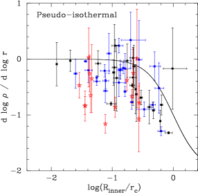
Figure 11: Solid line: logarithmic slope of the pseudo-isothermal model (equation 26). The data points are from observations of real galaxies (assuming a minimum stellar disk). Open circles: Verheijen (1997); filled circles: de Blok et al. (2001); filled squares: de Blok & Bosma (2002); stars: Swaters et al. (2003a). If these galaxies were described by the pseudo-isothermal model, they would follow the curve.

5 Summary

We have provided expressions to relate the half-mass radii of the Einasto and Prugniel-Simien models to a) the radius, $r_{-2}$, where the logarithmic slope of the density profile equals $-2$, b) the virial radius, $r_{\rm vir}$, and c) the radius where the associated circular velocity profile has its maximum value, $r_{\rm max}$.

We have shown the dependence of the ‘concentration’ terms $r_{\rm vir}/r_{-2}$ and $r_{\rm vir}/r_{\rm e}$ (and $r_{\rm vir}/R_{\rm e}$) on the ratio $\rho_{\rm e}/\langle\rho_{\rm univ}\rangle$, where $\rho_{\rm e}$ and $r_{\rm e}$ (and $R_{\rm e}$) are the Einasto (and Prugniel-Simien) scale density and half-mass radius. We also show how the slope of these models at $r_{\rm vir}$ depends solely on the ratio $\rho_{\rm e}/\langle\rho_{\rm univ}\rangle$ (Figure 3).

Over the radial range $10^{-2}<r/r_{-2}<4\times 10^{1}$, we have shown both the Einasto and Prugniel-Simien models possess the property that $\rho(r)/{\sigma(r)}^{3}$ can be roughly described by a power-law $r^{-\alpha}$ with the value of $\alpha$ slightly less than 2 for profile shapes $n$ equal to or greater than the best-fitting values reported both here and elsewhere.

Analytical expressions for the logarithmic slope of the Einasto and Prugniel-Simien models have been derived, and the slope expected from the inward extrapolation of these models, inside of $\sim$0.01 $r_{\rm vir}$, is compared with that from observations of real galaxies. The innermost ($r=0$) slope of the Prugniel-Simien model (0.73–0.87), as currently defined, appears too steep to match all the galaxy data, but agrees with theoretical expectations for a slope of $-0.75$ (Taylor & Navarro 2001) and $-0.78$ (Austin et al. 2005). Future work should explore the optimal value of the quantity $p$, the inner logarithmic profile slope in the Prugniel-Simien model. Setting $p=0$, one recovers the Einasto model, which appears capable of matching the inner profile slopes observed in real galaxies (Figure 10). Indeed, the typical value of $\sim-0.7$ at 0.1 kpc in our CDM halos agrees well with the galaxy data from Swaters et al. (2003a) and Simon et al. (2005), but is steeper than the value $-0.2\pm 0.2$ reported by de Blok et al. (2003) and others. We also note that, at present, the pseudo-isothermal model appears inconsistent with the galaxy data (Figure 11).

References

- (1) Abraham, R.G., Valdes, F., Yee, H.K.C., & van den Bergh, S. 1994, ApJ, 432, 75
- (2) An, J.H., & Evans, N.W. 2006, ApJ, 642, 752
- (3) Ascasibar, Y., Yepes, G., Gottlöber, S., & Müller, V, 2004, MNRAS, 352, 1109
- (4) Austin, C.G., Williams, L.L.R., Barnes, E.I., Babul, A., & Dalcanton, J.J. 2005, ApJ, 634, 756
- (5) Barnes, E.I., Williams, L.L.R., Babul, A., & Dalcanton, J.J. 2006, ApJ, 643, 797
- (6) Blais-Ouellette, S., Amram, P., Carignan, C., & Swaters, R. 2004, A&A, 420, 147
- (7) Bryan, G., & Norman, M. 1998, ApJ, 321, 80
- (8) Burkert, A. 1995, ApJ, 447, L25
- (9) Butcher, H., & Oemler, A. 1984, ApJ, 285, 426
- (10) Cardone, V.F., Piedipalumbo, E., & Tortora, C. 2005, MNRAS, 358, 1325
- (11) Coccato, L., Corsini, E.M., Pizzella, A., Morelli, L., Funes, J.G., & Bertola, F. 2004, A&A, 416, 507
- (12) de Blok, W.J.G. 2003, Proceedings IAU 220: Dark Matter in Galaxies, Eds. S.Ryder, D.J.Pisano, M.Walker, K.Freeman
- (13) de Blok, W.J.H. 2005, ApJ, 634, 227
- (14) de Blok, W.J.G., & Bosma, A. 2002, A&A, 385, 816
- (15) de Blok, W.J.G., Bosma, A., & McGaugh, S.S. 2003, MNRAS, 340, 657
- (16) de Blok, W.J.G., & McGaugh, S.S. 1997, MNRAS, 290, 533
- (17) de Blok, W.J.G., McGaugh, S.S., Rubin, V.C. 2001, AJ, 122, 2396
- (18) Dehnen, W., & McLaughlin, D.E. 2005, MNRAS, 363, 1057
- (19) Diemand, J., Moore, B., & Stadel, J. 2004, MNRAS, 353, 624
- (20) Diemand, J., Zemp, M., Moore, B., Stadel, J., & Carollo, M. 2005, MNRAS, 364, 665
- (21) Einasto, J. 1965, Trudy Inst. Astrofiz. Alma-Ata, 5, 87
- (22) Einasto, J. 1968, Tartu Astr. Obs. Publ. Vol. 36, Nr 5-6, 414
- (23) Einasto, J. 1969, Astrofizika, 5, 137
- (24) Einasto, J., & Haud, U. 1989, A&A, 223, 89
- (25) Fraser, C.W. 1972, The Observatory, 92, 51
- (26) Gentile, G., Burkert, A., Salucci, P., Klein, U., & Walter, F. 2006, ApJ, 634, L145
- (27) Goerdt, T., Moore, B., Read, J.I., Joachim, S/, & Zemp, M. 2006, MNRAS, 368, 1073
- (28) Graham, A.W. 2002, MNRAS, 334, 721
- (29) Graham, A.W., & Driver, S. 2005, PASA, 22(2), 118
- (30) Graham, A.W., Driver, S., Petrosian, V., Conselice, C.J., Bershady, M.A., Crawford, S.M., & Goto, T. 2005, AJ, 130, 1535
- (31) Graham, A.W., Trujillo, N., & Caon, N. 2001, AJ, 122, 1707
- (32) Hansen, S.H., & Stadel, J. 2006, Journal of Cosmology and Astro-Particle Physics, 5, 14
- (33) Hayashi, E., et al. 2004, MNRAS, 355, 794
- (34) Hernquist, L. 1990, ApJ, 356, 359
- (35) Kravtsov, A.V., Klypin, A.A., Bullock, J.S., & Primack, J.R. 1998, ApJ, 502, 48
- (36) Lavalle, J., et al. 2006, A&A, 450, 1
- (37) Lima Neto, G.B., Gerbal, D., & Márquez, I. 1999, MNRAS, 309, 481
- (38) Macciò, A.V., Murante, G., & Bonometto, S.P. 2003, ApJ, 588, 35
- (39) Mamon, G.A., & Łokas, E.L. 2005, MNRAS, 362, 95
- (40) Marchesini, D., D’Onghia, E., Chincarini, G., Firmani, C., Conconi, P., Molinari, E., & Zacchei, A. 2002, ApJ, 575, 801
- (41) Mashchenko, S., Couchman, H.M.P., & Wadsley, J. 2006, Nature, in press (astro-ph/0605672)
- (42) Merritt, D., Graham, A.W., Moore, B., Diemand, J., & Terzić, B. 2006, AJ, submitted (Paper I)
- (43) Merritt, D., Navarro, J.F., Ludlow, A., & Jenkins, A. 2005, ApJL, 624, L85
- (44) Moore, B., Quinn, T., Governato, F., Stadel, J., & Lake, G. 1999, MNRAS, 310, 1147
- (45) Navarro, J.F., Frenk, C.S., & White, S.D.M. 1995, MNRAS, 275, 720
- (46) Navarro, J.F., et al. 2004, MNRAS, 349, 1039
- (47) Okamura, S., Kodaira, K., & Watanabe, M. 1984, ApJ, 280, 7
- (48) Petrosian, V. 1976, ApJ, 209, L1
- (49) Prada, F., Klypin, A.A., Simonneau, E., & Betancort Rijo, J., Santiago, P., Gottlöber, S/ & Sanchez-Conde, M.A. 2006, ApJ, 645, 1001
- (50) Profumo, S., & Kamionkowski, M. 2006, Journal of Cosmology and Astro-Particle Physics, 3, 3
- (51) Prugniel, Ph., & Simien, F. 1997, A&A, 321, 111
- (52) Rasia, E., Tormen, G., & Moscardini, L. 2004, MNRAS, 351, 237
- (53) Rix, H.-W., Guhatakhurta, P., Colless, M.M., & Ing, K. 1997, MNRAS, 285, 779
- (54) Roberts, M.S., & Haynes, M.P. 1994, ARA&A, 32, 115
- (55) Salucci, P., & Burkert, A. 2000, ApJ, 537, L9
- (56) Sérsic, J.-L. 1963, Boletin de la Asociacion Argentina de Astronomia, vol.6, p.41
- (57) Sérsic, J.L. 1968, Atlas de galaxias australes
- (58) Simon, J.D., Bolatto, A.D., Leroy, A., & Blitz, L. 2003, ApJ, 596, 957
- (59) Simon, J.D., Bolatto, A.D., Leroy, A., & Blitz, L., Gates, E.L. 2005, ApJ, 621, 757
- (60) Sota, Y. Iguchi, O., Morikawa, M., Nakamichi, A. 2006, Proceedings of The Third 21COE Symposium : Astrophysics as Interdisciplinary Science (astro-ph/0512587)
- (61) Spekkens, K., Giovanelli, R., & Haynes, M. 2005, AJ, 129, 2119
- (62) Stoehr, F. 2006, MNRAS, 365, 147
- (63) Swaters, R.A., Madore, B.F., van den Bosch, F.C., & Balcells, M. 2003a, ApJ, 583, 732
- (64) Swaters, R.A., Verheijen, M.A.W., Bershady, M.A., & Andersen, D.R. 2003b, ApJ, 587, L19
- (65) Taylor, J.E., & Navarro, J.F. 2001, ApJ, 563, 483
- (66) Tenjes, P., Haud, U., & Einasto, J. 1994, A&A, 286, 753
- (67) Terzić, B., & Graham, A.W. 2005, MNRAS, 362, 197
- (68) Trujillo, I., Graham, A.W., & Caon, N. 2001, MNRAS, 326, 869
- (69) Valenzuela, O., Rhee, G., Klypin, A., Governato, F., Stinson, G., Quinn, T., & Wadsley, J. 2005, ApJ, submitted (astro-ph/0509644)
- (70) van den Bosch, F.C., Robertson, B.E., Dalcanton, J.J., & de Blok, W.J.G. 2000, AJ, 119, 1579
- (71) Verheijen, M.A. 1997, PhD thesis, Univ. of Groningen
- (72) Weinberg, M.D., & Katz, N. 2002, ApJ, 580, 627
- (73) Zhao, H.S. 1996, MNRAS, 278, 488