Inferring the emission regions for different kinds of gamma-ray bursts

Abstract

Using a theoretical model describing pulse shapes, we have clarified the relations between the observed pulses and their corresponding timescales, such as angular spreading time, dynamic time as well as cooling time. We find that the angular spreading timescale caused by curvature effect of fireball surface only contributes to the falling part of the observed pulses, while the dynamic one in the co-moving frame of the shell merely contributes to the rising portion of them provided the radiative time is negligible. In addition, the observed pulses resulted from the pure radiative cooling time of relativistic electrons exhibit the property of fast rise and slow decay (a quasi-FRED profile) together with smooth peaks. Besides, we interpret the phenomena of wider pules tending to be more asymmetric to be a consequence of the difference in emission regions. Meanwhile, we find the intrinsic emission time is decided by the ratios of lorentz factors and radii of the shells between short and long bursts. Based on the analysis of asymmetry, our results suggest that the long GRB pulses may occur in the regions with larger radius, while the short bursts could locate at the smaller distance from central engine.

Managing Editor

1 Introduction

Owing to possible overlapping between neighboring pulses, time profiles of gamma-ray bursts (GRBs) usually exhibit very diverse configurations¹⁸. Pulses as the fundamental elements of bursts provide us a clue which will help us catch their quiddities. According to the standard fireball shock model^19,33,15, the pulses are generally proposed to either originate from the internal shocks produced by collisions between different shells in the fireball^24,37 or come from the action of the external shock on the circum-burst medium^14,26,4,6. However, problems are still in existence not only for their radiation mechanisms but also at the aspect of the differences between short and long pulses in their profiles.

It had been pointed out that GRB light curves especially the pulses in them could reproduce the temporal activity of its inner engine^10,2,17. Dermer & Mitman⁵ had found that investigations on pulses were preferred for learning whether GRB sources require engines to be long-lasting or short-lived. The long-lasting central engine should produce more relativistic outflows during this phase which naturally lead to long-lasting emissions in the co-moving frame of the shells. The long time together with the delay time caused by the curvature effect of photosphere can inevitably results in longer duration in the observer frame^39,. Qin and Lu²³ thought that for most of observed pulses their corresponding co-moving pulses might contain a long decay time relative to the time-scale of the curvature effect. Moreover, studies with BATSE data for GRB pulses also indicate most sources do not display the curvature effects^11,1, which suggests that the physics of such pulse formation is dominated or determined by other effects, perhaps the hydrodynamic or radiative cooling process or both of them. It happens that the relations between these timescales and temporal structure of GRBs had been researched by some authors^27,29.

For the long and smooth single-peak GRBs, the curvature effects⁹ or external shock⁴ could be the leading action. The result that many short bursts are highly variable demonstrates short GRBs can’t be produced by external shocks¹⁶. So one of the aims in this work is to conjecture the approximate regions where bursts could occur. With this purpose, the structures of observed pulses connecting with different timescales are taken into account in very detail. These results suggest that short and long bursts might take place in different spatial regions from the sources.

2 Theoretical model

In this section we first introduce an analytic model based on the assumption of isotropic radiation in the frame of fireball^22,. The model has offered us a fundamental expression of pulses concerning observed counts flux (see paper II, eq. [21])

$$C(\tau)=C_{0}\frac{\int\limits_{\widetilde{\tau}_{\theta,min}}^{\widetilde{\tau}_{\theta,max}}\widetilde{I}(\tau_{\theta})(1+\beta\tau_{\theta})^{2}(1-\tau+\tau_{\theta})d\tau_{\theta}}{\Gamma^{3}(1-\beta)^{2}(1+\frac{\beta}{1-\beta}\tau)^{2}}\int\limits_{\nu_{1}}^{\nu_{2}}\frac{g_{0,\nu}(\nu_{0,\theta})}{\nu}d\nu$$ (1)

with

$$\tau=\frac{T-t_{c}-D/c+R_{c}/c}{R_{c}/c}$$ (2)

and

$$\tau_{\theta}=\frac{t_{\theta}-t_{c}}{R_{c}/c}$$ (3)

where $R_{c}$ and $\Gamma$ denote the corresponding initial radius of the fireball at time $t_{c}$ and the lorentz factor of ejecta when photons start emitting from the shocked shells, and $T$ and $t_{\theta}$ stand for the observation time by observer and the emission time from the photosphere respectively. $D$ is the luminosity distance from observer to the source. $\tau$ and $\tau_{\theta}$ are two dimensionless quantities and related by the following expression

$$\tau_{\theta}=\frac{\tau-(1-\mu)}{1-\beta\mu}$$ (4)

where $\mu=cos\theta$, and more detailed definitions of the relevant variables can be referred to paper I and II. Followed our recent work (paper I) the co-moving pulse form is assumed to be

$$\widetilde{I}(\tau_{\theta})\equiv I(\tau_{\theta})=I_{0}\left\{\begin{array}[]{cc}exp[(\tau_{\theta}-\tau_{\theta,0})/\sigma_{r}]&\ \ (\tau_{\theta,min}\leq\tau_{\theta}\leq\tau_{\theta,0})\\ exp[-(\tau_{\theta}-\tau_{\theta,0})/\sigma_{d}]&\ \ (\tau_{\theta,0}<\tau_{\theta}\leq\tau_{\theta,max})\\ \end{array}\right.$$

and let $\sigma_{r}/\sigma_{d}=\xi$.

From eq.(1), the one-to-one relation between $C(\tau)$ and $\tau$ can be constructed on condition that the values of the lorentz factor $\Gamma$ and the co-moving width $\Delta\tau_{\theta}=\tau_{\theta,max}-\tau_{\theta,min}$ have been assigned in advance.

3 Time scales

It has been known that the structure of GRB pulse is usually thought to be determined by three time scales. The first is angular spreading timescale, $T_{ang}\approx R_{c}/(2\Gamma^{2}c)$, which is caused by the interval between the arrival times of the photons emitted from different region of the shell²⁸. The second is dynamic timescale or shock shell-crossing time, $T_{dyn}\approx t_{dyn}^{{}^{\prime}}/2\Gamma$ with $t_{dyn}^{{}^{\prime}}=\Delta^{{}^{\prime}}/v_{sh}^{{}^{\prime}}$ in the rest frame of shell²⁵, where $\Delta^{{}^{\prime}}$ is the thickness of shell and $v_{sh}^{{}^{\prime}}$ is the velocity of shock relative to the pre-shocked flow. The last one is radiative generally synchrotron cooling time, $T_{syn}\simeq t_{\gamma}^{{}^{\prime}}/\Gamma$, where $t_{\gamma}^{{}^{\prime}}$ is the radiative timescale in co-moving frame of the shell³². As the duration the asymmetry of pulses (For convenience, we define the asymmetry in previous manner as the ratio of the rise fraction ($t_{r}$) of full width at half maximum ($FWHM$) of pulse to the decay fraction ($t_{d}$).) is likewise thought to be decided by the above three timescales.

Now, Let us consider an uniform and spherical shell moving outwards with a radial velocity of $v=c\beta$, which emits photons consecutively at different times as the shock propagates into it. The relation between observation time $T$ and the emitting time $t^{\prime}$ in co-moving frame of the shell has been gotten³¹ and can be written as

$$T\equiv(1-\beta\mu)t^{\prime}+(1-\mu)R_{c}/c=T_{int}+T_{ang}$$ (5)

where the first part of the right-hand side of the equation resulting from the time $t^{\prime}$ is defined as intrinsic timescale, and the second part is purely caused by the curvature effects. Assuming the distance of observer from the central engine is $D$, from equations (2), (4) and (5), one can verify the meaning of $T$ in eqs. (2) and (5) is identical if only I let the initial time at radius $R_{c}$ be constrained with $t_{c}=(R_{c}-D)/c.$ In this situation, I can get $t^{\prime}=\Delta\tau_{\theta}R_{c}/c$, where $\Delta\tau_{\theta}=\sigma_{r}+\sigma_{d}$ denotes the width of co-moving pulse (see paper I). Then I find that

$$T_{int}=(1-\beta\mu)t^{\prime}=(1-\beta\mu)\Delta\tau_{\theta}R_{c}/c$$ (6)

actually involves the contributions of timescales arising from co-moving frame to the pulse duration. In terms of the current fireball shock model, the intrinsic time $T_{int}$ (or $\Delta\tau_{\theta}$) is often interpreted as a consequence of combination of $T_{dyn}$ and $T_{syn}$.

4 Resulting pulses

We examine the dependence of the structure of pulses on the distinct timescales when parts of them are taken no account of due to some special physical reasons. Suppose the rising part of the co-moving pulse corresponds to the shell crossing time and its decay portion relates to the cooling time, we thus have the opportunity to distinguish their individual effects on the observed temporal profiles in the following extreme instances. In the internal shock model, pulses are caused by the dissipation of a fraction of kinetic energy of ejecta with lorentz factors that could exceed 100^8,19. In the following, we take $\Gamma=100$ as the representative value for the most sources.

4.1 Pulses dominated by $T_{ang}$

If the shell thickness $\Delta^{\prime}$ becomes thin enough due to the collision between the shell and the circum-burst medium at larger distance from the central engine, and/or the velocity of the forward shock is relativistic²⁶, the intrinsic time $T_{int}$ would be expected to be very small relative to $T_{ang}$. In this case, the effective timescales in eq. (5) are then reduced to be

$$T\approx T_{ang}=(1-\mu)R_{c}/c\approx R_{c}/2\Gamma^{2}c$$ (7)

in the case of $\Gamma\gg 1$.

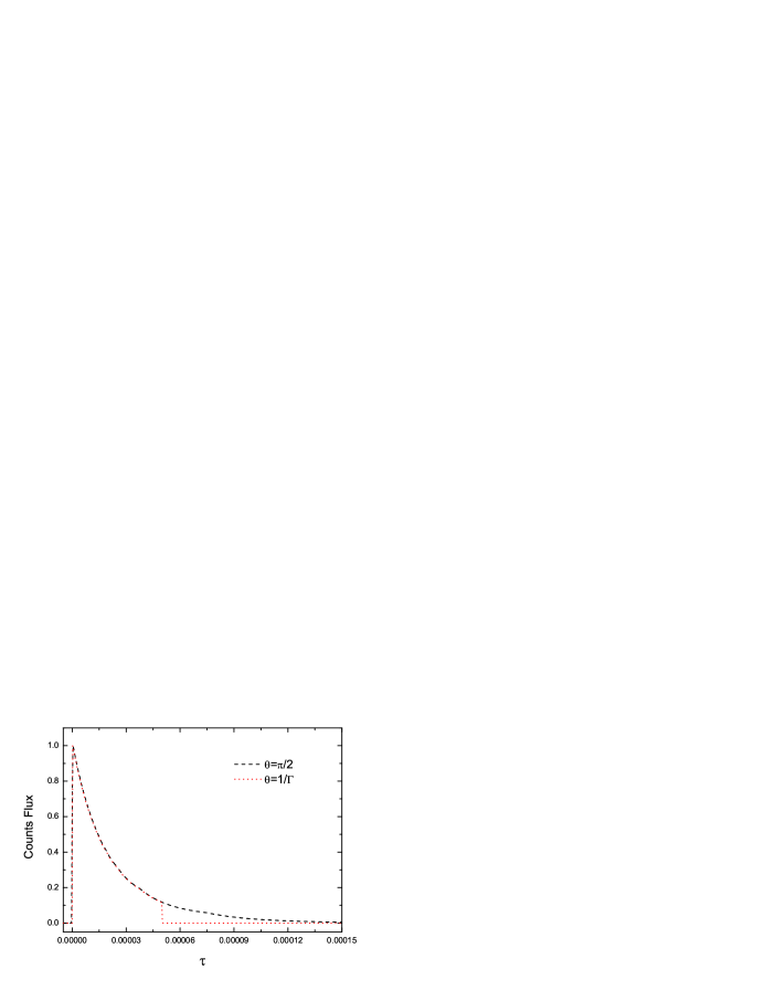
Figure 1: Plot of counts flux vs. $\tau$ for the normalized curves from angular spreading time, where we take $\Gamma=100$, $\Delta\tau_{\theta}=0.001$ and $R_{c}=10^{15}cm$. The dashed and dotted lines represent different emitting areas on the fireball surface and have been symbolized in the plot.

The resulting pulses have been displayed in figure 1. Here we can optionally appoint the value of $\xi$, say, for special $\xi=1$. In fact, our previous work (see, paper II) has concluded that the expected pulses are independent of their co-moving pulse shapes when their local width is narrow enough. We find from figure 1 that the pulses resulted from the angle spreading timescale behave the standard decay form in the shape, although they come from distinct surface. Furthermore, the discrepancy in the two durations demonstrates the contributions of photons from photosphere to light curves decrease with the reduction of the emitting area.

4.2 Pulses arising from $T_{dyn}$

Considering an ejecta moving towards us in the line of sight or beaming effect due to large lorentz factors in a small distance, the curvature effect on the observation might become very tiny. In the case of neglecting relativistic curvature effect (i.e. $\mu=1$), the dominant component of the duration $T$ in eq. (5) would remain to be

$$T\approx T_{int}=T_{dyn}=(1-\beta\mu)t^{\prime}\approx\Delta\tau_{\theta}R_{c}/2\Gamma^{2}c$$ (8)

where the $\Delta\tau_{\theta}$, $R_{c}$ and $\Gamma$ are taken some typical values as 10, $10^{13}cm$ and 100 respectively. To contrast the effects of diverse ratios between $\sigma_{r}$ and $\sigma_{d}$ on observed pulse shapes, we assign $\xi=3.0,5.7$ and $9.0$ correspondingly. Here the angle is taken as $\theta=1/(10^{5}\Gamma)$ so that it is ensured to be small enough. The current cases represent fast cooling physical process in co-moving frame of the shell.

In the following, for each pulses, the magnitude of count fluxes is normalized to a unit, and the relative time $\tau$ was re-scaled so that their right end of $FWHM$ is located at the same point. These normalized and re-scaled curves have been displayed in figure 2, from which we can find that the co-moving pulses with dominant dynamic timescales would lead to spiky analytic pulses. At the same time, the asymmetry of analytic pulses is proportional to the co-moving pulses’ ratio. In other words, with the increasing of dynamic timescale the observed pulses would become more asymmetric and show like exponential rise and fast decay (ERFD). Under extreme physical conditions, we shall draw the conclusion that the unmixed dynamic times should result in highly spiky pulses without decay portion.

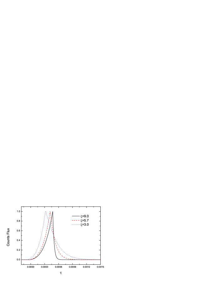
Figure 2: Plot of counts flux vs. $\tau$ for the normalized and re-scaled curves from dynamic timescale, where we take $\Gamma=100$, $\Delta\tau_{\theta}=10$, $R_{c}=10^{13}cm$ and $\theta=1/(10^{5}\Gamma)$. Different symbols have been shown in this plot.

4.3 Pulses originated from $T_{syn}$

As pointed by previous authors^32,30, the cooling time-scale is probably much larger than the above two time-scales, for instance, the accelerated particles radiate quite slowly, especially for very large radii due to the low densities of the shell¹⁷. It is thus necessary to reveal how the observed curves are influenced by the radiation of electrons. The cooling timescale can be expressed as follows

$$T\approx T_{int}=T_{syn}=(1-\beta\mu)t^{\prime}\approx\Delta\tau_{\theta}R_{c}/2\Gamma^{2}c$$ (9)

where the co-moving pulses must be mostly formed by its decay potion.

Resembling figure 2, the normalized and re-scaled curves from eq. (1) for different co-moving pulses’ ratios, say $\xi=1.0,0.3,0.1$, are similarly plotted in figure 3. On the occasions of $\xi\ll 1$, the analytic pulses are almost governed by radiative cooling time, namely considerably slow cooling process comparable to dynamical timescale of shocks crossing the shocked flows. From figure 3 we find the shapes of all these resulting curves in this case follow a form of fast rise and slow decay (quasi-FRED), and a profile of smooth instead of spiky peak. Additionally, with the increasing of cooling timescale the observed pulses would become more symmetric and smooth. Taking into account of an ultimate situation, $\xi=0$, we calculate the asymmetry of the resulting pulse and find it has an upper limit, here 0.37, when the parameters are assigned to be certain values such as $\Gamma=100$, $\Delta\tau_{\theta}=10$ and $R_{c}=10^{13}cm$. The theorem certainly holds for other curves from any of sets of parameters, provided the curves are completely contributed by the cooling time.

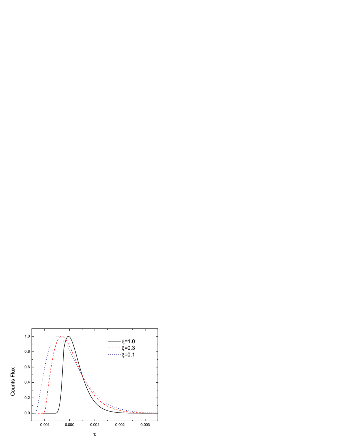
Figure 3: Plot of counts flux vs. $\tau$ for the normalized and re-scaled curves from radiative cooling time, where we take $\Gamma=100$, $\Delta\tau_{\theta}=10$, $R_{c}=10^{13}cm$ and $\theta=1/(10^{5}\Gamma)$. Different symbols have been shown in this plot.

5 Comparison between $T_{ang}$ and $T_{dyn}$

In fact, for most reasonable parameters the cooling time is much shorter than other physical timescales^27,10,19,34, especially in the scenario of internal shocks. In this case, $T_{ang}$ and $T_{dyn}$ could be the key factors acting on the properties of observed pulses. To discern which one is more significant than the other, I contrast the two timescales from eqs. (7) and (8) in figure 4. The reason for taking $\theta\sim 1/\Gamma$ in $T_{ang}$ is that the outflows crossed by internal shocks are generally assumed to be highly collimated.

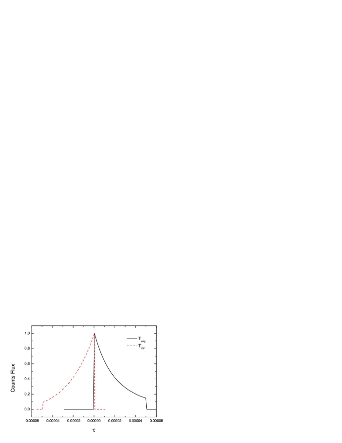
Figure 4: Contrasts between normalized and translated horizontally temporal profiles on timescales associated with the curvature effect, $T_{ang}$ with $\Gamma=100$, $R_{c}=10^{13}cm$, $\theta=1/\Gamma$ and $\Delta\tau_{\theta}=0.001$ and the shell-crossing time, $T_{dyn}$ with $\Gamma=100$, $R_{c}=10^{13}cm$, $\theta=1/(10^{5}\Gamma)$ and $\Delta\tau_{\theta}=1$. Symbols are denoted by solid line for angular spreading time and dashed line for dynamic time in this plot.

As is shown in figure 4, when the width of the rising co-moving pulse, $\Delta\tau_{\theta}$, becomes larger than 1 or the thickness of the shell is wide enough, the dynamic timescale would go beyond the the angular one. The opposite is the angular timescale could be the leading contribution to observations. If only the two timescales are comparable in this situation the observed pulses will be expected to be more symmetric. Or else, the pulses will show the characteristics of either FRED or ERFD shapes.

6 Independence of pulse shape on parameters

The above-mentioned timescales had been proved to be dependent on the radius, $R$, of the shell³². However, what we want to know now is how the pulses’ shape vary with the radius once the lorentz factors, the width as well as the ratio of co-moving pulses are definite for distinct radii. These analytic pulses are displayed in figure 5,

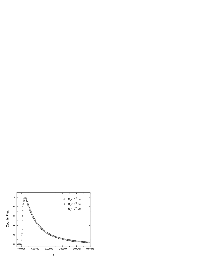
Figure 5: Profiles of the normalized analytic pulses in the observer frame, where I take $\Gamma=100$, $\theta=\pi/2$, $\Delta\tau_{\theta}=0.1$ and $\xi=1$. Curves for distinct radii are distinguished by triangles, circles and squares respectively. Symbols are marked in this plot.

in which we surprisingly see the pulses coming from different radii are undistinguishable in shape or asymmetry. The consistency manifests the curves are independent of radii on this occasion, which in turn shows the parameters, $\Gamma$, $\Delta\tau_{\theta}$ and $\xi$, or part of them, should evolve with radius rather than keep constant.

It had been known that the bulk Lorentz factor increases linearly with radius so long as the fireball is not baryon loaded and not complicated by non-spherical expansion⁷ until $\Gamma\sim 1000$ ^35,40, and then follows a $\Gamma\propto t^{-3/8}$ law ²¹. Unfortunately, the initial value of the shell width $\Delta^{{}^{\prime}}$ (or $t_{dyn}^{{}^{\prime}}$) together with its evolution with radius hasn’t been understood yet. I assume the co-moving width decreases with the increasing of radius, namely, $\Delta\tau_{\theta}\propto 1/R$, because of the violent interaction of the shells with circum-burst medium. For example, the lorentz factors are taken as $\Gamma=100,1000,10$ whose corresponding values of other parameters are $\Delta\tau_{\theta}=10,1,0.01$ and $R_{c}=10^{12}cm,10^{13}cm,10^{15}cm$ respectively. The expected pulses in observer frame are presented in figure 6, where they are identified by different symbols. Figure 6 seems to show the observed pulses arising from larger radius regions would be more asymmetric and be more close to the property of FRED. This might happen when the angular spreading time exceeds the dynamic one on condition that the two factors are considered.

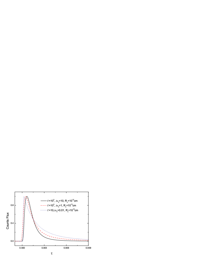
Figure 6: Plot of counts flux vs. $\tau$ for the normalized and re-scaled curves with the different sets of parameters of which their symbols have been shown in this plot. Besides, $\theta=\pi/2$ and $\xi=1$ are also designated.

7 Constraints on the intrinsic times

Once the cosmological effect is taken into account, the pulse duration should then be determined by

$$T_{dur}\sim(1+z)T\sim(1+z)(1+\Delta\tau_{\theta})R_{c}/2\Gamma^{2}c$$ (10)

where $z$ is the cosmological redshift for one given source. Previous investigations^3,42 had shown that the spectral lag is a direct consequence of spectral evolution. During the time interval of burst, in principal, the full photons emitted from distinct regions would contribute to the time lag. In the frame of internal shocks, the temporal and spectral features of pulses are probably governed by the hydrodynamics process instead of the curvature effect of the fireball surface³. In that case, the lag depends mainly on the dynamic timescale. On the other hand, either cooling time³⁰ or angular spreading time³¹ can also separately results in spectral lag. Although Ryde⁴³ has suggested the lag is mainly caused by the pulse decay-time, we here consider the whole contribution of the above three timescales to time lag lest additional errors could be produced. From eq.(10), we can easily get

$$\frac{T_{dur,s}}{T_{dur,l}}\sim\frac{(1+z_{s})(1+\Delta\tau_{\theta,s})R_{c,s}\Gamma_{l}^{2}}{(1+z_{l})(1+\Delta\tau_{\theta,l})R_{c,l}\Gamma_{s}^{2}}$$ (11)

where the subscripts $l$ and $s$ respectively denote long and short bursts.

Norris & Bonnell (2006) have shown the median lag is about 48  ms for long bursts and less than 1  ms for short ones. Assuming the leading contribution to pulse duration is the angular spreading time, $T_{\mathrm{dur}}\sim(1+z)R_{\mathrm{c}}/2\Gamma^{2}c$, i.e. lag, we can thus rewrite eq. (11) as

$$\frac{(1+z_{\mathrm{s}})\Gamma_{\mathrm{l}}^{2}}{(1+z_{\mathrm{l}})\Gamma_{\mathrm{s}}^{2}}\frac{(1+\Delta\tau_{\theta,\mathrm{s}})R_{\mathrm{c,s}}}{(1+\Delta\tau_{\theta,\mathrm{l}})R_{\mathrm{c,l}}}\leq\frac{1}{48}$$ (12)

where the median redshifts are respectively appointed to be $z_{\mathrm{s}}\simeq 0.5,\,z_{\mathrm{l}}\simeq 2.5$ for short and long bursts (Norris & Bonnell 2006). After submitting the values of redshift to eq.(12), one can derive

$$\frac{(1+\Delta\tau_{\theta,\mathrm{l}})R_{\mathrm{c,l}}}{(1+\Delta\tau_{\theta,\mathrm{s}})R_{\mathrm{c,s}}}\geq 20\frac{\Gamma_{\mathrm{l}}^{2}}{\Gamma_{\mathrm{s}}^{2}}$$ (13)

from which we can estimate the lower limit of lorentz factors for short bursts once the accurate limits of $\Gamma_{\mathrm{l}}$ can be well known. Some authors had determined the relatively exact value of the Lorentz factor for long GRBs, by using the reverse shock information, whose typical values range from 100 to 1000 ^e.g.51,52. However, the information of the local pulse width, $\Delta\tau_{\theta}$, and the radius, $R_{\mathrm{c}}$, hasn’t been achieved until now. Therefore, before this estimation, the width and the radius need to be reasonably assigned or assumed in advance. In particular, eq. (13) shows that the intrinsic time, $t^{\mathrm{{}^{\prime}}}=\Delta\tau_{\theta}R_{\mathrm{c}}/c$, is decided by the ratios of lorentz factors and radii of shells between short and long bursts.

8 Conclusion and discussion

By studying the influences of different timescales on the shape of pulses, we conclude that the profiles of observed pulses arising from angular spreading times would be long-tailed and called standard decay form without rising part, and those only resulting from dynamic timescales would follow a rising form. Which one is more dominant than another is determined by the value of $\Delta\tau_{\theta}$, i.e. $\Delta\tau_{\theta}>1$ for dynamic dominant case, and vice versa. The pure radiative cooling times would lead to smooth and FRED-like temporal profiles without too long tails. Additionally, we find the intrinsic emission time, $t^{\mathrm{{}^{\prime}}}$, is constrained by the ratios of lorentz factors and radii of the shells between short and long bursts.

Spada et al.³² found by simulating internal shocks that the angular spreading and the dynamic times are comparable when a shell broadens linearly in some special regions. When it happens, the thickness $\Delta^{{}^{\prime}}$ of the shell could be estimated by $\Delta^{{}^{\prime}}\sim R_{c}v^{\prime}_{sh}/(\Gamma c)$, which offer us a clue to understand that $T_{dyn}$ will go beyond $T_{ang}$ as $\Delta^{{}^{\prime}}\gg R_{c}v^{\prime}_{sh}/(\Gamma c)$. In this case, this conclusion just meet those previous viewpoints that the effect of not the geometry but the hydrodynamics governs the temporal and spectral characteristics of GRB pulses³. On the contrary, the component of duration from $T_{ang}$ would always be larger than from $T_{dyn}$ no matter how large the radii of fireball are.

On the other hand, for larger radii the radiative cooling time will be the dominant contribution to the pulse duration³², thus the shape of observed pulses should reflect the properties dominated by radiation during the whole duration. Moreover, the lorentz factors, thickness of the merged shell, the frequency of emitted photons and the energy equipartition factor $\varepsilon_{B}$ of the magnetic field will reduce to smaller values with the increasing of radii. On this occasion, there is a more strong contribution from $T_{syn}$ to observed pulses in contrast with either $T_{ang}$ or $T_{syn}$. Even if the outflows ejected from central engine are extremely calibrated in the early phase, the jet will spread sideways quickly²⁰ so that its geometry effects on observations are made to be more considerable. Therefore, the observed pulses are caused to exhibit more asymmetric and the trend of FRED are then strengthened.

We have known the leading model of central engine for long GRBs, perhaps including short ones, could be the collapsar model^36,38. Besides, other merger models of two compact objects have also been proposed^44,45,46,47. However, the analysis in this work is independent of the detailed progenitor models. The lorentz factors had been estimated as an order of 100-1000 for long bursts^51,52, while its lower limit is about 500 for short ones (Norris and Bonnell 2006). Meanwhile, we have reached a conclusion in our recent works^48,49 that the lorentz factors is proportional to $\Gamma^{-\omega}$ with $\omega>2$ for short bursts and $\omega<2$ for long bursts. In terms of the properties of tiny spectral lags in short bursts as well as their symmetric pulse characteristic, I thus infer that, although short and long GRB pulses could be interpreted with the same emission mechanism¹² in terms of the possible synchrotron radiation, the long and asymmetric FRED pulses could be produced by external shock in larger radii¹⁴, while the short and symmetric pulses might be formed by internal shock in smaller emission distance from sources. We expect it to be verified in the future by the SWIFT satellite in view of its capability of precise and prompt localization.

References

- [1] L. Borgonovo and F. Ryde, Astrophys. J. 548, 770 (2001).
- [2] F. Daigne and R. Mochkovitch, Mon. Not. R. Astron. Soc. 296, 275(1998)
- [3] F. Daigne and R. Mochkovitch, Mon. Not. R. Astron. Soc. 342, 587(2003)
- [4] C. D. Dermer, M. Böttcher and J. Chiang, Astrophys. J. 515, L49 (1999).
- [5] C. D. Dermer and K. E. Mitman, Third Rome Workshop on Gamma Ray Bursts in the Afterglow Era, ed. M. Feroci, F. Frontera, N. Masetti, & L. Piro (San Francisco: ASP), ASP Conf. Ser. 312, 301 (2004).
- [6] C. D. Dermer, Astrophys. J. 614, 284 (2004).
- [7] D. Eichler and A. Levinson, Astrophys. J. 529, 146 (2000).
- [8] E. E. Fenimore and R. Epstein, Astron. Astrophys. Suppl. S. 97, 59 (1993).
- [9] E. E. Fenimore, et al., Astrophys. J. 473, 998 (1996).
- [10] S. Kobayashi, T. Piran and R. Sari, Astrophys. J. 490, 92 (1997).
- [11] D. Kocevski, F. Ryde & E. Liang, Astrophys. J. 596, 389 (2003).
- [12] S. McBreen, F. Quilligan, B. McBreen, et al., Gamma-Ray Burst and Afterglow Astronomy 2001: A Workshop Celebrating the First Year of the HETE Mission. Am. Inst. Phys., New York, AIP Conf. Proc. 662, 290 (2003).
- [13] E. McMahon, P. Kumar & A. Panaitescu, Mon. Not. R. Astron. Soc. 354, 915(2004).
- [14] P. Mészáros and M. J. Rees, Astrophys. J. 405, 278 (1993).
- [15] P. Mészáros, Annu. Rev. Astron. Astr. 40, 137 (2002).
- [16] E. Nakar and T. Piran, Mon. Not. R. Astron. Soc. 330, 920 (2002a).
- [17] E. Nakar and T. Piran,Astrophys. J. 572, L139 (2002b).
- [18] J. P. Norris, et al.,Astrophys. J. 459, 393 (1996).
- [19] T. Piran, Phys. Rep+. 314, 575 (1999).
- [20] T. Piran, Sci. 295, 986 (2002).
- [21] T. Piran, 2005, astro-ph/0503060
- [22] Y. P. Qin, Z. B. Zhang, F. W. Zhang, et al., Astrophys. J. 617, 439 (2004). (Paper II)
- [23] Y. P. Qin and R. J. Lu, Mon. Not. R. Astron. Soc. 362, 1085 (2005).
- [24] M. J. Rees and P. & Mész áros, Astrophys. J. 430, L93 (1994).
- [25] F. Ryde and V. Petrosian, Astrophys. J. 578, 290 (2002).
- [26] R. Sari and T. Piran, AIP Conf. Proc. 384, 782 (1996).
- [27] R. Sari, R. Narayan and T. Piran, Astrophys. J. 473, 204 (1996).
- [28] R. Sari and T. Piran, Astrophys. J. 485, 270 (1997).
- [29] R. Sari and T. Piran, Astrophys. J. 455, L143 (1995).
- [30] B. Schaefer, Astrophys. J. 602, 306 (2004).
- [31] R. F. Shen, et al., Mon. Not. R. Astron. Soc. 362, 59 (2005).
- [32] M. Spada, A. Panaitescu and P. Mészáros, Astrophys. J. 537, 824 (2000).
- [33] J. van Paradijs, C. Kouveliotou, & R. A. M. J. Wijers, Annu. Rev. Astron. Astr. 38, 379 (2000).
- [34] B. Wu, and E. E. Fenimore, Astrophys. J. 535, L29 (2000).
- [35] E. Woods and A. Loeb, Astrophys. J. 453, 583 (1995).
- [36] S. E. Woosley and A. I. MacFadyen, Astron. Astrophys. Suppl. S. 138, 499 (1999).
- [37] B. Zhang and P. Mészáros,Int. J. Mod. Phys. A. 19, 2385 (2004).
- [38] W. Zhang, S. E. Woosley and A. I. MacFadyen, Astrophys. J. 586, 356 (2003).
- [39] Z. B. Zhang and Y. P. Qin, Mon. Not. R. Astron. Soc. 363, 1290 (2005). (Paper I)
- [40] E. Ramirez-Ruiz and E. E. Fenimore, Astrophys. J. 539, 712 (2000).
- [41] J. P. Norris and J. T. Bonnell, Astrophys. J., accepted, 2006, astro-ph/0601190
- [42] D. Kocevski and E. Liang, Astrophys. J. 594, 385 (2003).
- [43] F. Ryde Astron. Astrophys. 429, 869 (2005).
- [44] D. Eichler, M. Livio, T. Piran and D. N. Schramm, Nat. 340, 126 (1989).
- [45] B. Paczyński Acta. Astron. 41, 257 (1991).
- [46] R. Narayan, B. Paczyński and T. Piran Astrophys. J. 359, L83 (1992).
- [47] P. Mészáros and M. J. Rees, Astrophys. J. 397, 570 (1992).
- [48] Z. B. Zhang et al., Chinese. J. Astron. Ast., accepted, 2006, astro-ph/0603710
- [49] Z. B. Zhang et al., Mon. Not. R. Astron. Soc., 2006, submitted
- [50] B. Zhang et al., Astrophys. J., in press, 2005, astro-ph/0508321
- [51] X. Y. Wang, Z. G., Dai, T., Lu, Mon. Not. R. Astron. Soc. 319, 1159 (2000)
- [52] B. Zhang, S. Kobayashi, P. Mészáros, Astrophys. J. 595, 950 (2003)